Estimating Causal Structure Using Conditional DAG Models
Chris. J. Oates [email protected]
School of Mathematical and Physical Sciences University of Technology Sydney
NSW 2007, Australia
Jim Q. Smith [email protected]
Department of Statistics University of Warwick Coventry, CV4 7AL, UK
Sach Mukherjee [email protected]
German Center for Neurodegenerative Diseases (DZNE) 53175 Bonn, Germany
Editor:Samuel Kaski
Abstract
This paper considers inference of causal structure in a class of graphical models called conditional DAGs. These are directed acyclic graph (DAG) models with two kinds of variables, primary and secondary. The secondary variables are used to aid in the estimation of the structure of causal relationships between the primary variables. We prove that, under certain assumptions, such causal structure is identifiable from the joint observational distribution of the primary and secondary variables. We give causal semantics for the model class, put forward a score-based approach for estimation and establish consistency results. Empirical results demonstrate gains compared with formulations that treat all variables on an equal footing, or that ignore secondary variables. The methodology is motivated by applications in biology that involve multiple data types and is illustrated here using simulated data and in an analysis of molecular data from the Cancer Genome Atlas.
Keywords: Graphical Models, Causal Inference, Directed Acyclic Graphs, Instrumental Variables, Data Integration
1. Introduction
The fact that primary variables of direct interest are often part of a wider context, including additional secondary variables, presents challenges for graphical modelling and causal inference, since in general the secondary variables will not be independent and simply marginalising may introduce spurious dependencies (Evans and Richardson, 2014). Moti-vated by this observation, we define conditional DAG (CDAG) models and discuss their semantics. Nodes in a CDAG are of two kinds, corresponding to primary and secondary variables, and as detailed below the semantics of CDAGs allow causal inferences to be made about the primary variables (Yi)i∈V whilst accounting for the secondary variables (Xi)i∈W. To limit scope, we focus on the setting where each primary variable has a known cause among the secondary variables. Specifically we suppose there is a bijection φ : V → W, between the primary and secondary index sets V and W, such that for each i ∈ V a di-rect1 causal dependency X
φ(i) → Yi exists. Under explicit assumptions we show that such secondary variables can aid in causal inference for the primary variables, because known relationships between secondary and primary variables render “primary-to-primary” causal links of the formYi →Yj identifiable from joint data on primary and secondary variables. We put forward score-based estimators of CDAG structure that we show are asymptoti-cally consistent under certain conditions; importantly, independence assumptions on the secondary variables are not needed.
This work is motivated by current efforts in biology aimed at exploiting high-throughput data to better understand causal molecular mechanisms, such as those involved in gene regulation or protein signaling. A notable feature of molecular biology is the fact that some causal links are relatively clearly defined by known sequence specificity. For example, the DNA sequence has a causal influence on the level of corresponding mRNA; mRNAs have a causal influence on corresponding total protein levels; and total protein levels have a causal influence on levels of post-translationally modified protein. This means that in a study involving a certain molecular variable (a protein, say), a subset of the causal influences upon it may be clear at the outset (e.g. the corresponding mRNA) and typically it is the unknown influences that are the subject of the study. Then, it is natural to ask whether accounting for the known influences can aid in identification of the unknown influences. For example, if interest focuses on causal relationships between proteins, known mRNA-protein links could be exploited to aid in causal identification at the protein-protein level. We show below an example using protein data.
Our development of the CDAG can be considered dual to the acyclic directed mixed graphs (ADMGs) developed by Evans and Richardson (2014), in the sense that we inves-tigate conditioning as an alternative to marginalisation. In this respect our work mirrors recently developed undirected graphical models called conditional graphical models (CGMs; Liet al, 2012; Caiet al., 2013) In CGMs, Gaussian random variables (Yk)k∈V satisfy
Yi ⊥⊥Yj|(Yk)k∈V\{i,j},(Xk)k∈W if and only if (i, j)∈/ G (1)
where G is an undirected acyclic graph and (Xk)k∈W are auxiliary random variables that are conditioned upon. CGMs have recently been applied to gene expression data (Yi)i∈V. In that setting Zhang and Kim (2014) used single nucleotide polymorphisms (SNPs) as the
(Xi)i∈W, while Logsdon and Mezey (2010); Yin and Li (2011); Caiet al.(2013) used expres-sion qualitative trait loci (e-QTL) as the (Xi)i∈W. The latter work was recently extended to jointly estimate several such graphical models in Chunet al.(2013). Also in the context of undirected graphs, van Wieringen and van de Wiel (2014) recently considered encoding a bijection between DNA copy number and mRNA expression levels into inference. Our work complements these efforts by using directed models that are arguably more appropriate for causal inference (Pearl, 2009). Evans (2015) uses a similar directed graphical characterisa-tion and nomenclature. However, secondary variables in Evans (2015) are unobserved and can have multiple children in the set of primary variables, while ours are observed and have exactly one child among the primary variables. CDAGs are also related to instrumental variables and Mendelian randomisation approaches (Didelez and Sheehan, 2007) that we discuss below (Section 2.2).
CDAGs share some similarity with the influence diagrams (IDs) introduced by Dawid (2002) as an extension of DAGs that distinguish between variable nodes and decision nodes. This generalised the augmented DAGs of Spirtes et al. (2000); Lauritzen (2000); Pearl (2009) in which each variable node is associated with a decision node that represents an intervention on the corresponding variable. However, the semantics of IDs are not well suited to the scientific contexts that we consider, where secondary nodes represent variables to be observed, not the outcomes of decisions. The notion of a non-atomic intervention (Pearl, 2003), where many variables are intervened upon simultaneously, shares similarity with CDAGs in the sense that the secondary variables are in general non-independent. However again the semantics differ, since our secondary nodes represent random variables rather than interventions. In a different direction, Neto et al. (2010) recently observed that the use of e-QTL data (Xi)i∈W can help to identify causal relationships among gene expression levels (Yi)i∈V. However, Netoet al. (2010) require independence of the (Xi)i∈W; this is too restrictive for general settings, including in molecular biology, since the secondary variables will typically themselves be subject to regulation and far from independent. An important and novel aspect of our approach is that no independence or conditional independence assumptions need to be placed on the secondary variables in order to draw causal conclusions about the primary variables.
This paper begins in Sec. 2 by defining CDAGs and discussing identifiability of their structure from observational data on primary and secondary variables. Sufficient conditions are then given for consistent estimation of CDAG structure along with an algorithm based on integer linear programming. The methodology is illustrated in Section 3 on simulated data, including data sets that violate CDAG assumptions, and on protein data from cancer samples, the latter from the Cancer Genome Atlas (TCGA).
2. Methodology
Below we define CDAGS, study their theoretical properties and propose consistent estima-tors for CDAG structure.
2.1 A Statistical Framework for Conditional DAG Models
Specif-v1
w1 v2 w2
v3 w3
(a)
type index node variable primary i∈V vi∈N(V) Yi secondary i∈W wi ∈N(W) Xi
(b)
Figure 1: A conditional DAG model with primary nodesN(V) ={v1, v2, v3}and secondary nodes N(W) = {w1, w2, w3}. Here primary nodes represent primary random variables (Yi)i∈V and solid arrows correspond to a DAG G on these vertices. Square nodes are secondary variables (Xi)i∈W that, in the causal interpretation of CDAGs, represent known direct causes of the corresponding (Yi)i∈V (dashed arrows represent known relationships; the random variables (Xi)i∈W need not be independent). The name conditional DAG refers to the fact that conditional upon (Xi)i∈W, the solid arrows encode conditional independence relationships among the (Yi)i∈V.
ically, indices correspond to nodes in graphical models; this is signified by the notation
N(V) = {v1, . . . , vp} and N(W) = {w1, . . . , wp}. Each node vi ∈ N(V) corresponds to a primary RVYi and similarly each nodewi ∈N(W) corresponds to a secondary RV Xi.
Definition 1 (CDAG) Aconditional DAG(CDAG)G, with primary and secondary index sets V, W respectively and a bijection φ between them, is a DAG on the primary node set N(V) with additional directed edges from each secondary node wφ(i) ∈ N(W) to its corresponding primary nodevi ∈N(V).
In other words, a CDAG G has node set N(V)∪N(W) and an edge set that can be generated by starting with a DAG on the primary nodesN(V) and adding a directed edge from each secondary node in N(W) to its corresponding primary node in N(V), with the correspondence specified by the bijectionφ. An example of a CDAG is shown in Fig. 1a. To further distinguishV andW in the graphical representation we employ circular and square vertices respectively. In addition we use dashed lines to represent edges that are required by definition and must therefore be present in any CDAG G.
Since the DAG on the primary nodes N(V) is of particular interest, throughout we use
G to denote a DAG on N(V). We use G to denote the set of all possible DAGs with |V|
vertices. For notational clarity, and without loss of generality, below we take the bijection to simply be the identity map φ(i) = i. The parents of node vi in a DAG G are indexed by paG(i) ⊆V \ {i}. Write anG(S) for the ancestors of nodes S ⊆ N(V)∪N(W) in the CDAGG (which by definition includes the nodes inS). For disjoint sets of nodes A, B, C
in an undirected graph, we say that C separates A and B if every path between a node in
A and a node inB in the graph contains a node inC.
v1
w1 v2 w2
v3 w3
(a) Step (i)
v1
w1 v2 w2
v3 w3
(b) Step (ii)
v1
w1 v2 w2
v3 w3
(c) Step (iii)
v1
w1 v2 w2
v3 w3
(d) Step (iv)
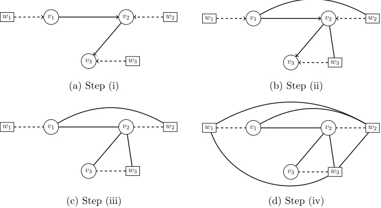
Figure 2: Illustratingc-separation. Here we ask whetherv3 and v1 arec-separated by {v2} in G, the CDAG shown in Fig. 1a. [Step (i): Take the subgraph induced by anG({v1, v2, v3}). Step (ii): Moralise this subgraph (i.e. join with an undirected edge any parents of a common child that are not already connected by a directed edge). Step (iii): Take the skeleton of the moralised subgraph (i.e. remove the arrowheads). Step (iv): Add an undirected edge between every pair (wi, wj). In the final panel (d) we ask whether there exists a path from v3 to v1 that does not pass throughv2; the answer is positive (e.g. v3−w3−w1−v1) and hence we conclude thatv3 6⊥⊥v1|v2[G], i.e. v3 and v1 are not c-separated by{v2}in G.]
A and B in the undirected graph U4 that is formed as follows: (i) Take the subgraph U1
induced by anG(A∪B∪C). (ii) Moralise U1 to obtainU2 (i.e. join with an undirected edge
any parents of a common child that are not already connected by a directed edge). (iii) Take the skeleton of the moralised subgraph U2 to obtain U3 (i.e. remove the arrowheads). (iv)
Add an undirected edge between every pair of nodes inN(W) to obtainU4.
The c-separation procedure is illustrated in Fig. 2, where we show that v3 is not c -separated fromv1 by the set{v2}in the CDAG from Fig. 1a.
Remark 3 The classical notion of d-separation for DAGs is equivalent to omitting step (iv) in c-separation. Notice that v3 is d-separated from v1 by the set {v2} in the DAG G,
underlining the need for a custom notion of separation for CDAGs.
The topology (i.e. the set of edges) of a CDAG carries formal (potentially causal) semantics on the primary RVs, conditional on the secondary RVs, as specified below. Write
Definition 4 (Independence model) The CDAGG, together withc-separation, implies a formal independence model(p.12 of Studen´y, 2005)
MG={hA, B|Ci ∈T(N(V)∪N(W)) :A⊥⊥B|C [G]} (2)
where hA, B|Ci ∈ MG carries the interpretation that the RVs corresponding to A are
con-ditionally independent of the RVs corresponding toB when given the RVs corresponding to
C. We will write A⊥⊥B|C [MG] as a shorthand for hA, B|Ci ∈ MG.
Remark 5 An independence modelMGdoes not contain any information on the structure of the marginal distribution P(Xi) of the secondary variables, due to the additional step (iv) in c-separation.
Lemma 6 (Equivalence classes) The map G7→ MG is an injection.
Proof Consider two distinct DAGsG, H ∈ G and suppose that, without loss of generality, the edge vi → vj belongs to G and not to H. It suffices to show that MG 6= MH. First notice that Grepresents the relations (i) wi6⊥⊥vj|wj [G], (ii)wi 6⊥⊥vj|wj,(vk)k∈V\{i,j}[G],
and (iii) wj ⊥⊥ vi|wi [G]. (These can each be directly verified by c-separation.) We show below thatHcannot also represent (i-iii) and hence, from Def. 4, it follows thatMG6=MH. We distinguish between two cases forH, namely (a)vi ←vj ∈/H, and (b)vi ←vj ∈H.
Case (a): Suppose (i) also holds forH; that is,wi6⊥⊥vj|wj [H]. Then sincevi →vj ∈/ H, it follows fromc-separation that the variablevimust be connected tovj by directed path(s) whose interior vertices must only belong to N(V)\ {vi, vj}. Thus H implies the relation
wi⊥⊥vj|wj,(vk)k∈V\{i,j} [H], so that (ii) cannot also hold.
Case (b): Since vi ←vj ∈H it follows from c-separation that wj 6⊥⊥vi|wi [H], so that (iii) does not hold forH.
Remark 7 More generally the same argument shows that a DAGG∈ G satisfiesvi→vj ∈/
G if and only if ∃S ⊆ paG(j)\ {i} such that wi ⊥⊥ vj|wj,(vk)k∈S [G]. As a consequence,
we have the interpretation that conditional upon the (secondary variables) (Xi)i∈W, the
solid arrows in Fig. 1a encode conditional independence relationships among the (primary variables) (Yi)i∈V, motivating the CDAG nomenclature.
Lemma 8 (Semi-graphoid) For any DAG G ∈ G, the set MG is semi-graphoid (Pearl and Paz, 1985). That is to say, for all disjoint A, B, C, D⊆N(V)∪N(W) we have
(i) (triviality)A⊥⊥ ∅|C[MG]
(ii) (symmetry) A⊥⊥B|C[MG] implies B⊥⊥A|C [MG]
(iii) (decomposition)A⊥⊥B, D|C [MG] implies A⊥⊥D|C[MG]
(iv) (weak union) A⊥⊥B, D|C[MG] implies A⊥⊥B|C, D[MG]
(v) (contraction) A⊥⊥B|C, D[MG]and A⊥⊥D|C [MG]implies A⊥⊥B, D|C[MG]
Proof The simplest proof is to note that our notion ofc-separation is equivalent to classical
d-separation applied to an extensionGof the CDAGG. The semi-graphoid properties then follow immediately by the facts that (i) d-separation satisfies the semi-graphoid properties (p.48 of Studen´y, 2005), and (ii) the restriction of a semi-graphoid to a subset of vertices is itself a semi-graphoid (p.14 of Studen´y, 2005).
Construct an extended graph G from the CDAG G by the addition of a node z and directed edges fromz to each of the secondary verticesN(W). Then for disjoint A, B, C⊆
N(V)∪N(W) we have thatAand B arec-separated byC inGif and only if Aand B are
d-separated by C inG. This is because every path in the undirected graph U4(G) (recall the definition of c-separation) that contains an edge wi → wj corresponds uniquely to a path inU3(G) that contains the sub-path wi →z→wj.
2.2 Causal CDAG Models
The previous section defined CDAG models using the framework of formal independence models. However, CDAGs can also be embellished with a causal interpretation, that we make explicit below. In this paper we make a causal sufficiency assumption that the (Xi)i∈W are the only source of confounding for the (Yi)i∈V and below we talk about direct causes at the level of (Xi)i∈W ∪(Yi)i∈V.
Definition 9 (Causal CDAG) A CDAG is causal when an edge vi → vj exists if and
only if Yi is a direct cause of Yj. It is further assumed that Xi is a direct cause of Yi and
not a direct cause of Yj for j 6=i. Finally it is assumed that noYi is a direct cause of any
Xj.
Remark 10 Here direct cause is understood to mean that the parent variable has a “con-trolled direct effect” on the child variable in the framework of Pearl (e.g. Def. 4.5.1 of Pearl, 2009) (it is not necessary that the effect is physically direct). No causal assumptions are placed on interaction between the secondary variables (Xi)i∈W.
Remark 11 In a causal CDAG the secondary variables(Xi)i∈W share some of the
proper-ties of instrumental variables (Didelez and Sheehan, 2007). Consider estimating the average causal effect of Yi on Yj. Then, conditioning on Xj in the following, Xi can be used as a
When we are interested in the controlled direct effect, we can repeat this argument with additional conditioning on the(Yk)k∈V\{i,j} (or a smaller subset of conditioning variables if the structure ofG is known).
2.3 Identifiability of CDAGs
There exist well-known identifiability results for independence models Mthat are induced by Bayesian networks; see for example Spirtes et al. (2000); Pearl (2009). These relate the observational distributionP(Yi)of the random variables (Y
i)i∈V to an appropriate DAG representation by means of d-separation, Markov and faithfulness assumptions (discussed below). The problem of identification for CDAGs is complicated by the fact that (i) the pri-mary variables (Yi)i∈V are insufficient for identification, (ii) the joint distributionP(Xi)∪(Yi)
of the primary variables (Yi)i∈V and the secondary variables (Xi)i∈W need not be Markov with respect to the CDAG G, and (iii) we must work with the alternative notion of c -separation. Below we propose novel “partial” Markov and faithfulness conditions that will permit, in the next section, an identifiability theorem for CDAGs. We make the standard assumption that there is no selection bias (for example by conditioning on common effects). We also assume throughout that there exists a true CDAGG. In other words, the observa-tional distributionP(Xi)∪(Yi) induces an independence model that can be expressed asMG for some DAGG∈ G.
Definition 12 (Partial Markov) Let Gdenote the true DAG. We say that the observa-tional distribution P(Xi)∪(Yi) is partially Markov with respect toGwhen the following holds:
For all disjoint subsets {i},{j}, C ⊆ {1, . . . , p} we have wi ⊥⊥ vj|wj,(vk)k∈C [MG] ⇒
Xi⊥⊥Yj|Xj,(Yk)k∈C.
Definition 13 (Partial faithfulness) Let G denote the true DAG. We say that the ob-servational distribution P(Xi)∪(Yi) is partially faithful with respect to G when the following
holds: For all disjoint subsets{i},{j}, C ⊆ {1, . . . , p}we havewi⊥⊥vj|wj,(vk)k∈C [MG]⇐
Xi⊥⊥Yj|Xj,(Yk)k∈C
Remark 14 The partial Markov property implies thatP(Xi)∪(Yi) admits the factorisation
p((xi)i=1,...,p,(yi)i=1,...,p) =p((xi)i=1,...,p) p
Y
i=1
p(yi|(yk)k∈paG(i), xi), (3)
while partial faithfulness ensures that none of the terms inside the product in Eqn. 3 can be further decomposed. In this work we will prove only estimation consistency; for more refined convergence analysis the partial faithfulness property must be strengthened. See e.g. Uhler et al. (2013) for a recent discussion of faithfulness in the DAG setting.
Remark 15 The partial Markov and partial faithfulness properties do not place any con-straint on the marginal distribution P(Xi) of the secondary variables.
The following is an immediate corollary of Lem. 6:
(i) It is not possible to identify the true DAG G based on the observational distribution
P(Yi) of the primary variables alone.
(ii) It is possible to identify the true DAG G based on the observational distribution
P(Xi)∪(Yi).
Proof (i) We have already seen thatP(Yi)is not Markov with respect to the DAGG: Indeed a statistical associationYi 6⊥⊥Yj|(Yk)k∈V\{i,j} observed in the distributionP(Yi)could either
be due to a direct interactionYi→Yj (orYj →Yi), or could be mediated entirely through variation in the secondary variables (Xk)k∈W. (ii) It follows immediately from Lemma 6 that observation of both the primary and secondary variables (Yi)i∈V ∪(Xi)i∈W is sufficient for identification ofG.
2.4 Estimating CDAGs From Data
In this section we assume that the partial Markov and partial faithfulness properties hold, so that the true DAGGis identifiable from the joint observational distribution of the primary and secondary variables. Below we consider score-based estimation for CDAGs and prove consistency of certain score-based CDAG estimators.
Definition 17 (Score function; Chickering (2003)) A score function is a map S :
G → [0,∞) with the interpretation that if two DAGs G, H ∈ G satisfy S(G) < S(H)
thenH is preferred to G.
We will study the asymptotic behaviour of ˆGS, the estimate of graph structure obtained by maximising S(G) over all G ∈ G based on observations (Xij, Yij)ji=1=1,...,p,...,n. Let Pn = P(X
j i,Y
j
i) denote the finite-dimensional distribution of the nobservations.
Definition 18 (Partial local consistency) We say the score function S is partially lo-cally consistent if, whenever H is constructed from G by the addition of one edgeYi →Yj,
we have
1. Xi 6⊥⊥Yj|Xj,(Yk)k∈paG(j)⇒limn→∞Pn[S(H)> S(G)] = 1 2. Xi ⊥⊥Yj|Xj,(Yk)k∈paG(j)⇒limn→∞Pn[S(H)< S(G)] = 1.
Theorem 19 (Consistency) If S is partially locally consistent then limn→∞Pn[ ˆGS =
G] = 1, so that GˆS is a consistent estimator of the true DAGG.
Proof It suffices to show that limn→∞Pn[ ˆGS =H] = 0 wheneverH 6=G. There are two cases to consider:
Case (a): Suppose vi → vj ∈ H butvi → vj ∈/ G. Let H0 be obtained from H by the removal ofvi →vj. Fromc-separation we havewi⊥⊥vj|wj,(vk)k∈paG(j)[G] and hence from
the partial Markov property we have Xi ⊥⊥Yj|Xj,(Yk)k∈paG(j). Therefore if S is partially
Case (b): Suppose vi → vj ∈/ H but vi → vj ∈ G. Let H0 be obtained from H by the addition of vi → vj. From c-separation we have wi 6⊥⊥ vj|wj,(vk)k∈paG(j) [G] and
hence from the partial faithfulness property we have Xi 6⊥⊥ Yj|Xj,(Yk)k∈paG(j). There-fore if S is partially locally consistent then limn→∞Pn[S(H) < S(H0)] = 1, so that limn→∞Pn[ ˆGS =H] = 0.
Remark 20 In this paper we adopt a maximum a posteriori (MAP) -Bayesian approach and consider score functions given by a posterior probabilityp(G|(xl
i, yil) l=1,...,n
i=1,...,p)of the DAG
Ggiven the data (xl i, yil)
l=1,...,n
i=1,...,p. This requires that a prior p(G) is specified over the spaceG
of DAGs. From the partial Markov property we have that, for nindependent observations, such score functions factorise as
S(G) =p(G) n
Y
l=1
p((xli)i=1,...,p) p
Y
i=1
p(yil|(ykl)k∈paG(i), xli). (4)
We further assume that the DAG priorp(G) factorises over parent sets paG(i)⊆V \ {i} as
p(G) = p
Y
i=1
p(paG(i)). (5)
This implies that the score function in Eqn. 4 is decomposable and the maximiser GˆS,
i.e. the MAP estimate, can be obtained via integer linear programming (ILP). In Sec. 2.6 we derive an ILP that targets the CDAG GˆS and thereby allows exact (i.e. deterministic)
estimation in this class of models.
Lemma 21 A score function of the form Eqn. 4 is partially locally consistent if and only if, whenever H is constructed from G by the addition of one edge vi →vj, we have
1. Xi 6⊥⊥Yj|Xj,(Yk)k∈paG(j)⇒limn→∞Pn[BH,G>1] = 1
2. Xi ⊥⊥Yj|Xj,(Yk)k∈paG(j)⇒limn→∞Pn[BH,G<1] = 1
where
BH,G =
p((Yl
j)l=1,...,n|(Ykl) l=1,...,n k∈paH(j),(X
l
j)l=1,...,n)
p((Yl
j)l=1,...,n|(Ykl) l=1,...,n k∈paG(j),(X
l
j)l=1,...,n)
(6)
is the Bayes factor between two competing local models paG(j) and paH(j).
2.5 Bayes Factors and Common Variables
The secondary variables (Xl
i)l=1,...,n are included in all models, and parameters relating to these variables should therefore share a common prior. Below we discuss a formulation of the Bayesian linear model that is suitable for CDAGs. Consider variable selection for node
j and candidate parent (index) set paG(j) =π⊆V \ {j}. We construct a linear model for the observations
Yjl= [1Xjl]β0+Yπlβπ+lj, lj ∼N(0, σ2) (7)
whereYl
π = (Ykl)k∈π is used to denote a row vector and the noiselj is assumed independent forj = 1, . . . , p and l= 1, . . . , n. Although suppressed in the notation, the parameters β0,
βπ and σ are specific to nodej. This regression model can be written in vectorised form as
Yj =M0β0+Yπβπ+ (8)
where M0 is the n×2 matrix whose rows are the [1 Xjl] for l = 1, . . . , n and Yπ is the matrix whose rows are Yπl forl= 1, . . . , n.
We orthogonalize the regression problem by definingMπ = (I−M0(M0TM0)−1M0T)Yπ so that the model can be written as
Yj =M0β˜0+Mπβ˜π + (9)
where ˜β0 and ˜βπ are Fisher orthogonal parameters (see Deltell, 2011, for details). In the conventional approach of Jeffreys (1961), the prior distribution is taken as
pj,π( ˜βπ,β˜0, σ) = pj,π( ˜βπ|β˜0, σ)pj( ˜β0, σ) (10)
pj( ˜β0, σ) ∝ σ−1 (11)
where Eqn. 11 is the reference or independent Jeffreys prior. (For simplicity of exposition we leave conditioning upon M0, and Mπ implicit.) The use of the reference prior here is motivated by the observation that the common parameters β0, σ have the same meaning in each model π for variable Yj and should therefore share a common prior distribution (Jeffreys, 1961). Alternatively, the prior can be motivated by invariance arguments that derive p(β0, σ) as a right Haar measure (Bayarri et al., 2012). Note however that σ does not carry the same meaning acrossj∈V in the application that we consider below, so that the prior is specific to fixed j. For the parameter prior pj,π( ˜βπ|β˜0, σ) we use the g-prior (Zellner, 1986)
˜
βπ|β˜0, j, π∼N(0, gσ2(MπTMπ)−1) (12)
where g is a positive constant to be specified. Due to orthogonalisation, cov( ˆβπ) =
σ2(MT
πMπ)−1 where ˆβπ is the maximum likelihood estimator for ˜βπ, so that the prior is specified on the correct length scale (Deltell, 2011). We note that many alternatives to Eqn. 12 are available in the literature (including Johnson and Rossell, 2010; Bayarriet al., 2012). For discrete data we mention recent work by Massam and Weso lowski (2014).
Under the prior specification above, the marginal likelihood for a candidate modelπhas the following closed-form expression:
pj(yj|π) = 1 2Γ
n−2
2
1
π(n−2)/2
1
|MT
0 M0|1/2
1
g+ 1
|π|/2
b−(n−2)/2 (13)
b = yTj
I−M0(M0TM0)−1M0T − g
g+ 1Mπ(M
T
πMπ)−1MπT
Following Scott and Berger (2010), we control multiplicity via the prior
p(π)∝
p
|π|
−1
. (15)
Proposition 22 (Consistency) Let g =n. Then the Bayesian score function S(G) de-fined above is partially locally consistent, and hence the corresponding estimatorGˆS is
con-sistent.
Proof This result is an immediate consequence of Lemma 21 and the well-known variable selection consistency property for the unit-information g-prior (see e.g. Fern´andez et al., 2001).
2.6 Computation via Integer Linear Programming
Structure learning for DAGs is a well-studied problem, with contributions including Fried-man and Koller (2003); Silander and Myllym¨akki (2006); Tsamardinoset al.(2006); Cowell (2009); Cussens (2011); Yuan and Malone (2013). Discrete optimisation via ILP can be used to allow efficient estimation for graphical models, exploiting the availability of power-ful (and exact) ILP solvers (Nemhauser and Wolsey, 1988; Wolsey, 1998; Achterberg, 2009), as discussed in Bartlett and Cussens (2013). Below we extend the ILP approach to CDAG models.
We begin by computing and caching the quantities
p((yil)l=1,...,n|(ykl)kl=1∈π,...,n,(xli)l=1,...,n) (16) that summarise evidence in the data for the local model paG(i) =π ⊆V \ {i} for variable
i. These cached quantities are transformed to obtain “local scores”
s(i, π) := log(p((yil)l=1,...,n|(ykl)kl=1∈π,...,n,(xli)l=1,...,n)) + log(p(π)). (17) These are the (log-) evidence from Eqn. 16 with an additional penalty term that provides multiplicity correction over varyingπ⊆V\ {i}, arising from Eqn. 5. Then we define binary indicator variables that form the basis of our ILP as follows:
Π(i, π) := [paG(i) =π] ∀i= 1, . . . , p, π⊆V \ {i}. (18)
The information in the variables Π contains all information on the DAGG. However it will be necessary to impose constraints that ensure the Π correspond to a well-defined DAG:
X
π⊆V\{i}
Π(i, π) = 1 ∀i= 1, . . . , p (C1; convexity)
Constraint (C1) requires that every node i has exactly one parent set (i.e. there is a well-defined graph G). To ensureGis acyclic we require further constraints:
X
i∈C
X
π⊆V\{i}
π∩C=∅
(C2) states that for every non-empty set C there must be at least one node inC that does not have a parent inC.
Proposition 23 The MAP estimateGˆS is characterised as the solution of the ILP
ˆ
GS = arg maxG∈G
p
X
i=1
X
π⊆V\{i}
s(i, π)Π(i, π) (19)
subject to constraints (C1) and (C2).
Proof It was proven in Jaakolaet al. (2010) that (C1) and (C2) together exactly charac-terise the space G of DAGs.
For the applications in this paper, all ILP instances were solved using the GOBNILP software that is freely available to download from http://www.cs.york.ac.uk/aig/sw/
gobnilp/.
3. Results
Below we present results based on simulated data and data from molecular biology.
3.1 Simulated Data
We simulated data from linear-Gaussian structural equation models (SEMs). Here we sum-marise the simulation procedure, with full details provided in the supplement. We first sampled a DAG Gfor the primary variables and a second DAG G0 for the secondary vari-ables (independently of G), following a sampling procedure described in the supplement. That is,Gis the causal structure of interest, whileG0 governs dependence between the
sec-ondary variables. Data for the secsec-ondary variables (Xi)i∈W were generated from an SEM with structureG0. The strength of dependence between secondary variables was controlled by a parameterθ∈[0,1]. Hereθ= 0 renders the secondary variables independent andθ= 1 corresponds to a deterministic relationship between secondary variables, with intermediate values of θ giving different degrees of covariation among the secondary variables. Finally, conditional on the (Xi)i∈W, we simulated data for the primary variables (Yi)i∈V from an SEM with structureG. To manage computational burden, for all estimators we considered only models of size|π| ≤5. Performance was quantified by the structural Hamming distance (SHD) between the estimated DAG ˆGS and true, data-generating DAGG, taking into ac-count directionality; we report the mean SHD as computed over 10 independent realisations of the data. We emphasise that the secondary variables need not be generated from a DAG model, however this is a convenient and familiar approach. We note that in the biological application below a DAG for the secondary variables might not be appropriate.
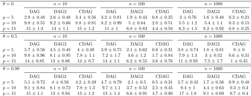
In Table 1 we compare the proposed score-based CDAG estimator with the correspond-ing score-based DAG estimator that uses only the primary variable data (Yl
θ= 0 n= 10 n= 100 n= 1000
DAG DAG2 CDAG DAG DAG2 CDAG DAG DAG2 CDAG
p= 5 2.9±0.48 2.6±0.48 3.4±0.56 3.2±0.81 1.9±0.43 0.8±0.25 3±0.76 1.6±0.48 0.3±0.21
p= 10 9.8±0.55 9.2±0.66 8.8±0.81 8.2±0.99 5±0.84 2.8±0.51 5.5±1.2 5.4±1.1 0.3±0.15
p= 15 15±1.3 14±1.1 15±1.2 11±1 6.8±0.83 4.4±0.58 6.3±1.5 8.2±0.92 0.8±0.25
θ= 0.5 n= 10 n= 100 n= 1000
DAG DAG2 CDAG DAG DAG2 CDAG DAG DAG2 CDAG
p= 5 5.7±0.56 4.5±0.48 4±0.49 3.9±0.75 2.1±0.62 0.6±0.31 3.8±0.74 1.8±0.81 0±0
p= 10 9.8±0.96 8.1±0.95 7.8±1.1 7.2±1.7 4.6±1.2 1.7±0.84 7.9±1.3 3±0.52 0.6±0.31
p= 15 14±0.85 13±0.86 13±0.7 14±1.1 6.2±0.55 3.6±0.76 11±0.93 7.5±1.7 1±0.45
θ= 0.99 n= 10 n= 100 n= 1000
DAG DAG2 CDAG DAG DAG2 CDAG DAG DAG2 CDAG
p= 5 5.1±0.72 4±0.56 4.2±0.49 4.7±0.79 2.1±0.5 0.5±0.31 2.7±0.42 1.7±0.56 0.9±0.48
p= 10 9.1±0.84 8.1±0.72 7.8±1.3 9.7±1.1 3.7±0.52 2.5±0.45 9.4±1 4.4±0.64 0.3±0.3
p= 15 15±1.1 13±0.94 13±1.2 13±1.4 6.6±0.91 4.7±0.86 17±1.8 9.1±0.69 0.7±0.4
Table 1: Simulated data results. Here we display the mean structural Hamming distance from the estimated to the true graph structure, computed over 10 independent realisations, along with corresponding standard errors. [Data were generated using linear-Gaussian structural equations. θ∈[0,1] quantifies dependence between the secondary variables (Xi)i∈W,nis the number of data points andpis the number of primary variables (Yi)i∈V. “DAG” = estimation based only on primary variables (Yi)i∈V, “DAG2” = estimation based on the full data (Xi)i∈W∪(Yi)i∈V, “CDAG” = estimation based on the full data and enforcing CDAG structure.]
and strong covariation among the secondary variables. In each data-generating regime we found that CDAGs were either competitive with, or (typically) more effective than, the DAG and DAG2 estimators. In the p = 15, n = 1000 regime (that is closest to the bio-logical application that we present below) the CDAG estimator dramatically outperforms these two alternatives. Inference using DAG2 and CDAG (that both use primary as well as secondary variables) is robust to large values of θ, whereas in thep= 15, n= 1000 regime, the performance of the DAG estimator based on only the primary variables deteriorates for large θ. This agrees with intuition since association between the secondary Xi’s may induce correlations between the primaryYi’s. CDAGs outperformed DAG2 at largen (see also Table 1).
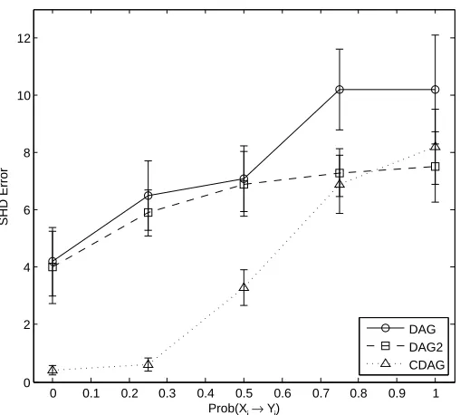
To better understand the limitations of CDAGs we considered three data-generating regimes that violate the CDAG assumptions. Firstly we focused on the θ = 0, p = 15,
n= 1000 regime where the CDAG estimator performs well when data are generated “from the model”. We then introduced a numberE of edges of the formXi →Yj whereYi →Yj ∈
0 0.1 0.2 0.3 0.4 0.5 0.6 0.7 0.8 0.9 1 0
2 4 6 8 10 12
Prob(X i→ Yj)
SHD Error
DAG DAG2 CDAG
Figure 3: Simulated data results; model misspecification. [Data were generated using linear-Gaussian structural equations. Here we fixed θ = 0, p = 15, n = 1000 and considered varying the number E of misspecified edges as described in the main text. On thex-axis we display the marginal probability that any given edgeYi →
Yj has an associated misspecified edgeXi →Yj, so that when Prob(Xi →Yj) = 1 the numberE of misspecified edges is equal to the number of edges inG. “DAG” = estimation based only on primary variables (Yi)i∈V, “DAG2” = estimation based on the full data (Xi)i∈W∪(Yi)i∈V, “CDAG” = CDAG estimation based on the full data (Xi)i∈W ∪(Yi)i∈V.]
down to 0%. At 0% the partial faithfulness assumption is violated and estimators are no longer consistent. Results (SFig. 1) show that CDAG remains effective over a wide range of data-generating regimes, but eventually degrades when faithfulness is strictly violated. Thirdly, we considered removing the Xi → Yi dependence from a random subset of the indices i∈ {1, . . . , p}, so that faithfulness is violated in a more heterogeneous way across the CDAG, similar to the situation considered by Neto et al. (2010). Results (SFig. 2) showed CDAG remained effective when only a handful of deletions occur, but eventually degraded as all the dependencies on secondary variables were removed.
3.2 Molecular Biological Data
protein node variable CHK1 wi Xi p-CHK1 vi Yi CHK2 wj Xj p-CHK2 vj Yj
(a)
v1
w1
v2
w2 ?
?
(b)
Y versus Yj i
OVCA−like
X | Xi j
versus Y
j
| Xj
X | Xj i
versus Y
i
| Xi
CHK1PS345 vs CHK1
CHK2PT68 vs CHK2
BRCA−like UCEC/BLCA−like HNSC/LUAD/LUSC−like GBM−like COAD/READ−like M KIRC−like
(c)
Figure 4: CHK1 total protein (t-CHK1) as a natural experiment for phosphorylation of CHK2 (p-CHK2). (a) Description of the variables. (b) A portion of the CDAG relating to these variables. It is desired to estimate whether there is a causal relationshipYi → Yj (possibly mediated by other protein species) or vice versa. (c) Top row: Plotting phosphorylated CHK1 (p-CHK1;Yi) against p-CHK2 (Yj) we observe weak correlation in some of the cancer subtypes. Middle row: We plot the residuals when t-CHK1 is regressed on total CHK2 (t-CHK2; x-axis) against the residuals when p-CHK2 is regressed on t-CHK2 (y-axis). The plots show a strong (partial) correlation in each subtype that suggests a causal effect in the direction p-CHK1 → p-CHK2. Bottom row: Reproducing the above but with the roles of CHK1 and CHK2 reversed, we see much reduced and in many cases negligible partial correlation, suggesting lack of a causal effect in the reverse direction, i.e. p-CHK18p-CHK2. [The grey line in each panel is a least-squares linear regression.]
Nelander et al., 2008; Hillet al., 2012; Oates and Mukherjee, 2012). Aberrations to causal signalling networks are central to cancer biology (Weinberg, 2013).
X4EBP1PS65
AKTPS473 AMPKPT172
CRAFPS338
CHK1PS345
CHK2PT68
ERALPHAPS118
GSK3ALPHABETAPS21S9
HER2PY1248 MAPKPT202Y204
MEK1PS217S221
P27PT157
P38PT180Y182
P70S6KPT389 PKCALPHAPS657
S6PS235S236
SRCPY416
JNKPT183Y185
MTORPS2448
EGFRPY1068 FOXO3APS318S321
P90RSKPT359S363
RICTORPT1135
TUBERINPT1462
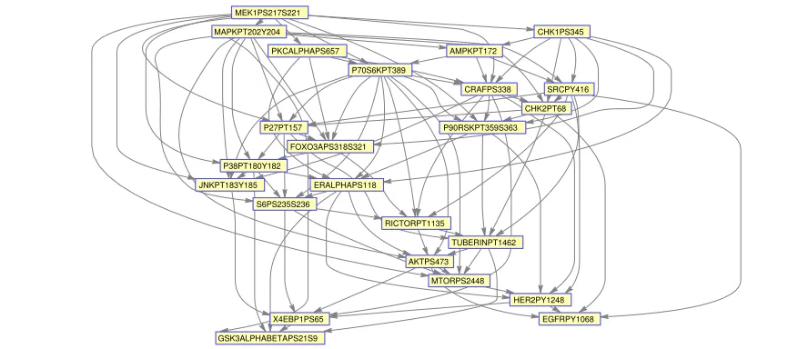
Figure 5: Maximum a posterioriconditional DAG, estimated from protein data from cancer samples (from the Cancer Genome Atlas, samples belonging to the BRCA-like group, see text). Here vertices represent phosphorylated proteins (primary vari-ables) and edges have the biochemical interpretation that the parent protein plays a causal role in phosphorylation of the child protein.
method described in Sec. 3.1 may not be suitable for use here since thet-proteins are likely confounded by unobserved variables.
The data we analyse are from the TCGA “pan-cancer” project (Akbani et al., 2014) and comprise measurements of protein levels (including both t- and p-proteins) using a technology called reverse phase protein arrays (RPPAs). We focus on p = 24 proteins for which (total, phosphorylated) pairs are available; the data span eight different cancer types (as defined by a clustering analysis due to St¨adler et al., 2015) with a total sample size of
n= 3,467 patients. We first illustrate the key idea of using secondary variables to inform causal inference regarding primary variables with an example from these data:
Example 1 (CHK1 t-protein as a natural experiment for CHK2 phosphorylation)
Consider RVs (Yi, Yj) corresponding respectively to p-CHK1 and p-CHK2, the
phosphory-lated forms of CHK1 and CHK2 proteins. Fig. 4c (top row) shows that these variables are weakly correlated in most of the 8 cancer subtypes. There is a strong partial correla-tion between t-CHK1 (Xi) and p-CHK2 (Yj) in each of the subtypes when conditioning on
t-CHK2 (Xj) (middle row), but there is essentially no partial correlation between t-CHK2
(Xj) and p-CHK1 (Yi) in the same subtypes when conditioning on t-CHK1 (bottom row).
Thus, under the CDAG assumptions, this suggests that there exists a directed causal path from p-CHK1 to p-CHK2, but not vice versa.
40 50 60 70 80 90 100 40
50 60 70 80 90 100
Num. edges (DAG)
Num. edges (CDAG)
OVCA−like BRCA−like
UCEC/BLCA−like
HNSC/LUAD/LUSC−like
GBM−like COAD/READ−like
M
KIRC−like
Figure 6: Cancer patient data; relative density of estimated protein networks. Here we plot the number of edges in the networks inferred by estimators based on DAGs (x-axis) and based on CDAGs (y-axis). [Each point corresponds to a cancer subtype (see text). “DAG” = estimation based only on primary variables (Yi)i∈V, “CDAG” = estimation based on the full data and enforcing CDAG structure.]
We now apply the CDAG methodology to allp= 24 primary variables that we consider, using data from the largest subtype in the study (namely BRCA-like). The estimated graph is shown in Fig. 5. We note that assessment of the biological validity of this causal graph is a nontrivial matter, and outside the scope of the present paper. However, we observe that several well known edges, such as from p-MEK to p-MAPK, appear in the estimated graph and are oriented in the expected direction. Interestingly, in several of these cases, the edge orientation is different when a standard DAG estimator is applied to the same data, showing that the CDAG formulation can reverse edge orientation with respect to a classical DAG (see supplement). We note also that the CDAG is denser, with more edges, than the DAG (Fig. 6), demonstrating that in many cases, accounting for secondary variables can render candidate edges more salient. These differences support our theoretical results insofar as they demonstrate that in practice CDAG estimation can give quite different results from a DAG analysis of the same primary variables but we note that proper assessment of estimated causal structure in this setting is beyond the scope of this paper.
4. Conclusions
work we put forward CDAGs as a simple class of graphical models that make this distinction explicit. Motivated by molecular biological applications, we developed CDAGs that use bijections between primary and secondary index sets. The general approach presented here could be extended to other multivariate settings where variables are in some sense non-exchangeable. Naturally many of the philosophical considerations and practical limitations and caveats of classical DAGs remain relevant for CDAGs and we refer the reader to Dawid (2010) for an illuminating discussion of these issues.
The application to biological data presented above represents a principled approach to integrate different molecular data types (here, total and phosphorylated protein, but the ideas are general) for causal inference. Our results suggest that integration in a causal framework may be useful in some settings. Theoretical and empirical results showed that CDAGs can improve estimation of causal structure relative to classical DAGs when the CDAG assumptions are even approximately satisfied.
We briefly mention three natural extensions of the present work: (i) The CDAGs put forward here allow exactly one secondary variable Xi for each primary variable Yi. In many settings this may be overly restrictive. In biology there are many examples of known causal relationships that are one-to-many or many-to-one. It would be natural to extend CDAGs in this direction. Examples of a more general formulation along these lines were recently discussed by Netoet al. (2010) in the context of eQTL data. Conversely we could extend the recent ideas of Kang et al.(2014) by allowing for multiple secondary variables for each primary variable, not all of which may be valid as instruments. (ii) In many applications data may be available from multiple related but causally non-identical groups, for example disease types. It could then be useful to consider joint estimation of multiple CDAGs, following recent work on estimation for multiple DAGs (Oateset al., 2015, 2014). (iii) Biotechnological advances now mean that the number pof variables is frequently very large. Estimation for high-dimensional CDAGs may be possible using recent results for high-dimensional DAGs (e.g. Kalisch and B¨uhlmann, 2007; Loh and B¨uhlmann, 2014, and others).
Acknowledgments
This work was inspired by discussions with Jonas Peters at the WorkshopStatistics for Com-plex Networks, Eindhoven 2013, and Vanessa Didelez at theUK Causal Inference Meeting, Cambridge 2014. CJO was supported by the Centre for Research in Statistical Methodology (CRiSM) EPSRC EP/D002060/1 and the ARC Centre of Excellence for Mathematical and Statistical Frontiers. Part of this work was done while SM was at the Medical Research Council Biostatistics Unit and University of Cambridge, Cambridge, UK. SM acknowledges the support of the Medical Research Council and a Wolfson Research Merit Award from the UK Royal Society.
References
Akbani, R.et al.(2014). A pan-cancer proteomic perspective on The Cancer Genome Atlas.
Nature Communications 5:3887.
Bartlett, M., and Cussens, J. (2013). Advances in Bayesian network learning using integer programming. Proceedings of the 29th Conference on Uncertainty in Artificial Intelli-gence, 182-191.
Bayarri, M. J., Berger, J. O., Forte, A., and Garc´ıa-Donato, G. (2012). Criteria for Bayesian model choice with application to variable selection.The Annals of Statistics 40(3), 1550-1577.
Cai, T. T., Li, H., Liu, W., and Xie, J. (2013). Covariate-adjusted precision matrix estima-tion with an applicaestima-tion in genetical genomics.Biometrika 100(1), 139-156.
Cai, X., Bazerque, J. A., and Giannakis, G. B. (2013). Inference of gene regulatory networks with sparse structural equation models exploiting genetic perturbations.PLoS Computa-tional Biology9(5), e1003068.
Chickering, D.M. (2003). Optimal structure identification with greedy search.The Journal of Machine Learning Research 3, 507-554.
Chun, H., Chen, M., Li, B., and Zhao, H. (2013). Joint conditional Gaussian graphical models with multiple sources of genomic data. Frontiers in Genetics4, 294.
Consonni, G., and La Rocca, L. (2010). Moment priors for Bayesian model choice with applications to directed acyclic graphs. Bayesian Statistics9(9), 119-144.
Cowell, R.G. (2009). Efficient maximum likelihood pedigree reconstruction.Theoretical Pop-ulation Biology 76, 285-291.
Cussens, J. (2011). Bayesian network learning with cutting planes.Proceedings of the 27th Conference on Uncertainty in Artificial Intelligence, 153-160.
Dawid, A.P. (2001). Separoids: A mathematical framework for conditional independence and irrelevance. The Annals of Mathematics and Artificial Intelligence 32(1-4), 335-372.
Dawid, A.P. (2002). Influence diagrams for causal modelling and inference. International Statistical Review 70(2), 161-189.
Dawid, A.P. (2010). Beware of the DAG!Journal of Machine Learning Research-Proceedings Track 6, 59-86.
Deltell, A.F. (2011). Objective Bayes criteria for variable selection. Doctoral dissertation, Universitat de Val`encia.
Didelez, V., and Sheehan, N. (2007). Mendelian randomization as an instrumental variable approach to causal inference. Statistical Methods in Medical Research 16, 309-330.
Evans, R. J. (2015). Margins of discrete Bayesian networks. arXiv:1501.02103.
Fern´andez, C., Ley, E., and Steel, M. F. (2001). Benchmark priors for Bayesian model averaging. Journal of Econometrics100(2), 381-427.
Friedman, N., and Koller, D. (2003). Being Bayesian about network structure: A Bayesian approach to structure discovery in Bayesian networks. Machine Learning50(1-2):95-126.
Greenland, S. (2000). An introduction to instrumental variables for epidemiologists. Inter-national Journal of Epidemiology 29(4), 722-729.
Hill, S. M., Lu, Y., Molina, J., Heiser, L. M., Spellman, P. T., Speed, T. P., Gray, J. W., Mills, G. B., and Mukherjee, S. (2012). Bayesian inference of signaling network topology in a cancer cell line. Bioinformatics28(21), 2804-2810.
Jaakkola, T., Sontag, D., Globerson, A., and Meila, M. (2010). Learning Bayesian net-work structure using LP relaxations.Proceedings of the 13th International Conference on Artificial Intelligence and Statistics, 358-365.
Jeffreys, H. (1961). Theory of probability. Oxford University Press, 3rd edition.
Johnson V.E., and Rossell D. (2010). Non-local prior densities for default Bayesian hypoth-esis tests.Journal of the Royal Statistical Society B 72, 143-170.
Kalisch, M., and B¨uhlmann, P. (2007). Estimating high-dimensional directed acyclic graphs with the PC-algorithm.Journal of Machine Learning Research8, 613-636.
Kang, H., Zhang, A., Cai, T. T., and Small, D. S. (2014). Instrumental variables esti-mation with some invalid instruments and its application to Mendelian randomization. arXiv:1401.5755.
Lauritzen, S.L. (2000). Causal inference from graphical models. In: Complex Stochastic Systems, Eds. O.E. Barndorff-Nielsen, D.R. Cox and C. Kl¨uppelberg.CRC Press, London.
Lauritzen, S.L., and Richardson, T.S. (2002). Chain graph models and their causal inter-pretations.Journal of the Royal Statistical Society: Series B 64(3):321-348.
Li, B., Chun, H., and Zhao, H. (2012). Sparse estimation of conditional graphical mod-els with application to gene networks. Journal of the American Statistical Association
107(497), 152-167.
Logsdon, B. A., and Mezey, J. (2010). Gene expression network reconstruction by convex feature selection when incorporating genetic perturbations.PLoS Computational Biology
6(12), e1001014.
Loh, P. L., and B¨uhlmann, P. (2014). High-dimensional learning of linear causal networks via inverse covariance estimation. Journal of Machine Learning Research15, 3065-3105.
Nelander, S., Wang, W., Nilsson, B., She, Q. B., Pratilas, C., Rosen, N., Gennemark, P., and Sander, C. (2008). Models from experiments: combinatorial drug perturbations of cancer cells.Molecular Systems Biology 4, 216.
Nemhauser, G.L., and Wolsey, L.A. (1988). Integer and combinatorial optimization.Wiley, New York.
Neto, E. C., Keller, M. P., Attie, A. D., and Yandell, B. S. (2010). Causal graphical models in systems genetics: a unified framework for joint inference of causal network and genetic architecture for correlated phenotypes. The Annals of Applied Statistics4(1), 320-339.
Oates, C. J., and Mukherjee, S. (2012). Network inference and biological dynamics. The Annals of Applied Statistics 6(3), 1209-1235.
Oates, C. J., Costa, L., and Nichols, T.E. (2014). Towards a multi-subject analysis of neural connectivity. Neural Computation 27, 1-20.
Oates, C. J., Smith, J. Q., Mukherjee, S., and Cussens, J. (2015). Exact estimation of multiple directed acyclic graphs. Statistics and Computing, to appear.
Pearl, J., and Paz, A. (1985). Graphoids: A graph-based logic for reasoning about relevance relations. Computer Science Department, University of California.
Pearl, J., and Verma, T. (1987). The logic of representing dependencies by directed graphs. In: Proceedings of the AAAI, Seattle WA, 374-379.
Pearl, J. (2003). Reply to Woodward. Economics and Philosophy19(2), 341-344.
Pearl, J. (2009).Causality: models, reasoning and inference (2nd ed.). Cambridge University Press.
Sachs, K., Perez, O., Pe’er, D., Lauffenburger, D. A., and Nolan, G. P. (2005). Causal protein-signaling networks derived from multiparameter single-cell data. Science
308(5721), 523-529.
Scott, J. G., and Berger, J. O. (2010). Bayes and empirical-Bayes multiplicity adjustment in the variable-selection problem. The Annals of Statistics38(5), 2587-2619.
Silander, T., and Myllym¨akki, P. (2006). A simple approach to finding the globally optimal Bayesian network structure.Proceedings of the 22nd Conference on Artificial Intelligence, 445-452.
Spirtes, P., Glymour, C., and Scheines, R. (2000).Causation, prediction, and search (Second ed.). MIT Press.
St¨adler, N., Dondelinger, F., Hill, S. M., Kwok, P., Ng, S., Akbani, R., Werner, H. M. J., Shahmoradgoli, M., Lu, Y., Mills, G. B., and Mukherjee, S. (2015). In preparation.
Tsamardinos, I., Brown, L.E., and Aliferis, C.F. (2006). The max-min hill-climbing Bayesian network structure learning algorithm. Machine Learning65(1), 31-78.
Uhler, C., Raskutti, G., Bhlmann, P., and Yu, B. (2013). Geometry of the faithfulness assumption in causal inference.The Annals of Statistics 41(2), 436-463.
van Wieringen, W. N., and van de Wiel, M. A. (2014). Penalized differential pathway analy-sis of integrative oncogenomics studies.Statistical Applications in Genetics and Molecular Biology 13(2), 141-158.
Weinberg, R. (2013). The biology of cancer. Garland Science.
Wolsey, L.A. (1998). Integer programming. Wiley, New York.
Yin, J., and Li, H. (2011). A sparse conditional Gaussian graphical model for analysis of genetical genomics data.The Annals of Applied Statistics 5(4), 2630-2650.
Yuan, C., and Malone, B. (2013). Learning optimal Bayesian networks: A shortest path perspective. Journal of Artificial Intelligence Research48, 23-65.
Zellner, A. (1986). On assessing prior distributions and Bayesian regression analysis with g-prior distributions. In A. Zellner, ed., Bayesian Inference and Decision techniques: Essays in Honour of Bruno de Finetti, Edward Elgar Publishing Limited, 389-399.