Effects of Generalized Fundamental Solution (GFS) on Generalized Integral Representation Method (GIRM)

Published online March 12, 2015 (http://www.sciencepublishinggroup.com/j/acm) doi: 10.11648/j.acm.s.2015040301.13

ISSN: 2328-5605 (Print); ISSN: 2328-5613 (Online)

Effects of Generalized Fundamental Solution (GFS) on

Generalized Integral Representation Method (GIRM)

Hiroshi Isshiki

IMA, Institute of Mathematical Analysis, Osaka, Japan

Email address:

[email protected]

To cite this article:

Hiroshi Isshiki. Effects of Generalized Fundamental Solution (GFS) on Generalized Integral Representation Method (GIRM). Applied and Computational Mathematics. Special Issue: Integral Representation Method and its Generalization. Vol. 4, No. 3-1, 2015, pp. 40-51. doi: 10.11648/j.acm.s.2015040301.13

Abstract:

Integral Representation Method (IRM) is one of convenient methods to solve Initial and Boundary Value Problems (IBVP). It can be applied to irregular mesh, and the solution is stable and accurate. IRM is developed to Generalized Integral Representation Method (GIRM) to treat any kinds of problems including nonlinear problems. In GIRM, Generalized Fundamental Solution (GFS) is used instead of Fundamental Solution (FS) in IRM. Since GFS is not limited to one, the effects of individual GFSs must be clarified. The continuity of GFS is related to the characteristics of individual GFSs.

Keywords:

Initial and Boundary Value Problems (IBVP), Integral Representation Method (IRM),

Generalized Integral Representation Method (GIRM), Generalized Fundamental Solution (GFS)

1. Introduction

Integral Representation Method (IRM) [1-3] is one of convenient methods to solve Initial and Boundary Value Problems (IBVP). It can be applied to irregular mesh, and the solution is stable and accurate. IRM was originally developed to solve linear boundary value problems, and the Fundamental Solution (FS) of the original differential equation plays a major role in IRM. IRM is developed to Generalized Integral Representation Method (GIRM) [4-7] to treat any kinds of problems including nonlinear problems. GIRM uses Generalized Fundamental Solution (GFS). GFS is not required to satisfy the differential equation of the original problem. We can use various GFSs for an individual problem.

Since GIRM is not limited to one, the effects of individual GFSs must be clarified. The continuity of GFS is related to the characteristics of individual GFSs. For example, in one-dimensional case, GFSs with discontinuous and continuous slopes show quite different property. Furthermore, the degree of continuity has important effects on the property.

GIRM is classified into 1-Step and 2-Step GIRMs. The effects of the continuity of GFS are different between 1-Step and 2-Step GIRMs. Since 1-Step GIRM is impossible for multi-dimensional convective problems, 2-Step GIRM is very important for the problems. For simplicity, we discuss one-dimensional advective diffusion problems in the present

paper.

2. Initial and Boundary Vale Problem

(IBVP) and Generalized Integral

Representation Method (GIRM)

2.1. Most Basic Problems

For simplicity, we discuss one-dimensional problems. The following five cases would be the most basic problems to discuss Initial and Boundary Value Problems (IBVP):

(a) Pure advection problem:

0

= ∂ ∂ + ∂ ∂

x C U t C

in −L<x<L for t>0, (1)

where C(x,t) and U are concentration of substance and advection velocity in region −L<x<L, respectively. The dependent variables t and x refer to time and space coordinate, respectively.

(b) Pure convection problem:

0

= ∂ ∂ + ∂ ∂

x u u t u

where u(x,t) is velocity of fluid flow. (c) Pure diffusion problem:

2 2 x C t C ∂ ∂ = ∂ ∂ _κ

in −L<x<L for t>0, (3)

where κ is coefficient of diffusion. (d) Diffusion problem in advection:

2 2 x C x C U t C ∂ ∂ = ∂ ∂ + ∂ ∂ _κ

in −L<x<L for t>0. (4)

(e) Diffusion problem in convection or Burgers’ equation:

2 2 x u x u u t u ∂ ∂ = ∂ ∂ + ∂ ∂ _κ

in −L<x<L for t>0. (5)

The boundary and initial conditions are given by

L g t L u C − = −       ) ,

( , Lt g L

u C + = +       ) ,

( for t>0, (6)

) ( ) 0 ,

(x f x u C =      

in −L<x<+L, (7)

respectively, where g−L and g+L are given constants, and

) (x

f is a given function.

We must notice the difference of the fundamental characteristics of advection, convection and diffusion. 2.2. 1-Stept GIRM

We discuss numerical solutions of Initial and Boundary Value Problem (IBVP) of advective diffusion. For simplicity, the discussions are confined to the one-dimensional problems. The differential equation, boundary condition and initial condition are given by Eqs. (4), (6) and (7), respectively.

We summarize One-Step Generalized Integral Representation Method (1-Step GIRM) [7]. Multiplying a function G~(x,ξ) of x and ξ on both side of Eq. (4)

∫

₋+       ∂ ∂ − ∂ ∂ + ∂ ∂ = L

L _x G x dx

t x C x t x C U t t x C ) , ( ~ ) , ( ) , ( ) , ( 0 ₂ 2 ξ κ

∫

∫

₋+ − ₋+ ∂ _∂ ∂ ∂ = L L L

L _x dx

x G t x C U dx x G t t x

C ~( , )

) , ( ) , ( ~ ) ,

( _ξ ξ

[

]

x L

L x L

L _x dx UC x t G x

x G t x

C =₌₋

+ − _∂ + ∂ −

_∫

( , ) ( , )~( , ) ~ ) , ( ₂ 2 ξ ξ κ L x L x x x G t x C x G x t x C = − =         ∂ ∂ − ∂ ∂ − ( , ) ~ ) , ( ) , ( ~ ) ,

( _ξ ξ

κ . (8)

Rewriting Eq. (8) and exchanging

x

and

ξ

, we obtain

∫

∫

₋+ = ₋+ ∂ _∂ ∂ ∂ L L L L d x G t C U d x G t t C _ξ ξ ξ ξ ξ ξ

ξ ~( , )

) , ( ) , ( ~ ) , (

[

]

L

L L

L d UC t G x

x G t

C =₌+₋

+

− _∂ −

∂

+κ

_∫

ξ _ξ(ξ, ) ξ (ξ, )~(ξ, )ξξ

~ ) , ( ₂ 2 L L x G t C x G t

C =+

− =         ∂ ∂ − ∂ ∂ + ξ ξ ξ ξ ξ ξ ξ ξ

κ ( , ) ~( , ) ( , ) ~( , ) . (9)

where G~(x,ξ) is a Generalized Fundamental Solution (GFS) chosen properly, for example, Gaussian GFS:

      ₋ −

= ₂ 2

2 ) ( exp 2 1 ) , ( ~ γ ξ γ π ξ x x

G (10)

Equation (9) is a generalized integral representation of Eq. (4). This integral representation is applied to numerical solution. If we know C(x,t) in −L≤x≤L, Eq. (9) is an integral equation with unknowns ∂C(x,t) ∂t in −L<x<L,

) , ( Lt

Cx − and Cx(L,t) , where G(x,ξ) is the kernel

function of the integral equation. Namely, we can obtain

)

,

(

x

t

C

numerically, if we use, for example, the following explicit time evolution process:

Let C(x,t) be known at time t

→

Obtain ∂C(x,t) ∂t from Eq. (9)

→

Then C(x,t+dt)=C(x,t)+dt∂C(x,t) ∂t

→

Add dt to t

→

Repeat. (11) 2.3. 2-Step GIRM

Now, we summarize Two-Step Generalized Integral Representation Method (2-Step GIRM) [7]. We rewrite the basic equations Eq. (4) as follows:

Non-uniformity equation: x C ∂ ∂ =

θ . (12)

Constitutive equation:

θ κ

− =

q . (13) Equilibrium equation: x q x C U t C ∂ ∂ − = ∂ ∂ + ∂ ∂

. (14)

Multiplying G~(x,ξ) on the both sides of Eq. (12) and integrating in region −L<x<L, we obtain

∫

₋+       ∂ ∂ − = L

L _x G x dx

t x C t

x,) ( , ) ~( , ) (

∫

∫

₋+ + ₋+

= L

L L

LG x xt dx C xt (x, )dx

~ ) , ( ) , ( ) , ( ~ ξ δ θ ξ ,

[

C(+L,t)G~(+L,ξ)−C(−L,t)G~(−L,ξ)

]

− (15)

where ) , ( ~ ) , ( ~ ξ δ ξ x x x G ₌ ∂ ∂

. (16)

Rewriting Eq. (15) and exchanging x and ξ, we obtain a generalized integral representation for Eq. (12):

∫

∫∫∫

=− ₋+L

L

VGξ xθ ξ t dξ C ξ t δ(ξ,x)dξ

~ ) , ( ) , ( ) , ( ~

[

G~(+L,x)C(+L,t)−G~(−L,x)C(−L,t)

]

+ . (17)

A generalized integral representation of Eq. (14) is obtained similarly. Multiplying G~(x,ξ) on the both sides of Eq. (14) and integrating in region −L<x<L, we obtain

∫

₋+ _∂ _∂ + ∂ _∂ +∂ _∂ _

= L

L _x dx

t x q x t x C U t t x C x

G~( , ) ( , ) ( , ) ( ,)

0 ξ

∫

₋+ ∂ _∂

= L

L _t dx

t x C x

G~( ,ξ) ( , )

∫

∫

−+ + − − − L L L

LU x t C x t x dx q x t (x, )dx

~ ) , ( ) , ( ~ ) , ( ) ,

( δ ξ δ ξ

[

G~(+L, )U(+L,t)C(+L,t)−G~(−L, )U(−L,t)C(−L,t)

]

+ ξ ξ

[

G~(+L, )q(+L,t)−G~(−L, )q(−L,t)

]

+ ξ ξ . (18)

Rewriting Eq. (18) and exchanging x and ξ, we obtain a generalized integral representation of Eq. (14):

[

]

∫

∫

₋+ = ₋+ + ∂ ∂ L L L

L _t d U tC t q t x d

t C x

G~(ξ, ) (ξ,) ξ (ξ,) (ξ,) (ξ,)δ~(ξ, ) ξ

[

G~(+L,x)U(+L,t)C(+L,t)−G~(−L,x)U(−L,t)C(−L,t)

]

−

[

G~(+L,x)q(+L,t)−G~(−L,x)q(−L,t)

]

− . (19)

Then, we can obtain C(x,t) numerically, if we use, for example, the following explicit time evolution process:

Let C(x,t) be known at time t

→

Obtain θ(x,t) from Eq. (17)

→

Obtain q(x,t) from Eq. (13)

→

Obtain ∂C(x,t) ∂t from Eq. (19)

→

Then C(x,t+dt)=C(x,t)+dt∂C(x,t) ∂t

→

Add

dt

to t

→

Repeat. (20)

3. Generalized Fundamental Solution

(GFS)

In one-dimension, we can consider various kinds of GFSs. The most basic GFS are Harmonic and Gaussian GFSs. In the following, we classify GFSs by the continuity.

3.1.

C

0 Continuous GFS

3.1.1. Harmonic GFS

| | 2 1 ) , (

~ _{ξ = −ξ}

x x

G , (21a)

) sgn( 2 1 ) , ( ~ ξ

ξ _{= −}

∂ ∂ x x x G

, (21b)

) ( ) , ( ~ 2 2 ξ δ

ξ _{= −}

∂ ∂ x x x G

, (21c)

where δ is Dirac’s delta function. G~(x,ξ) is called harmonic GFS, since it is the one-dimensional fundamental solution of Laplace operator:

⋯ + ∂ ∂ + ∂ ∂ = ∇ y x 2 2 2 2 2

. (22)

3.1.2. Triangle GFS

     > ≤       − − − = γ γ γξ γ ξ | | , 0 | | , 1 | | 4 ) , ( ~ 2 x x x x

G , (23a)

     < ≤ −       − − − = ∂ ∂ γ γ ξ γ ξ ξ | | , 0 | | ), sgn( 1 | | 2 1 ) , ( ~ x x x x x x

G _{, (23b)}

     > ≤ − + − = ∂ ∂ γ γ ξ δ γ ξ } | , 0 | | ), ( 2 1 ) , ( ~ 2 2 x x x x x G

. (23c)

3.1.3. Exponential GFS

      ₋ − − = γ ξ γ

ξ exp | |

2 ) , ( ~ x x

G , (24a)

) sgn( | | exp 2 1 ) , ( ~ ξ γ ξ ξ ₋       ₋ − = ∂ ∂ x x x x

G _{, (24b)}

) ( | | exp 2 1 ) , ( ~ 2 2 ξ δ γ ξ γ

ξ _{+ −}

     ₋ − − = ∂ ∂ x x x x

G _{. (24c)}

3.1.4. 0

C Gaussian GFS

      ₋ − − = 2 2 2 ) ( exp | | 5 . 0 ) , ( ~ γξ ξ

ξ x x

x

        ₋ − ⋅ ⋅       − − − − = ∂ ∂ 2 2 2 2 ) ( exp | | ) ( 5 . 0 ) sgn( 5 . 0 ) , ( ~ γ ξ ξ ξ γ ξ ξ x x x x x x G

, (25b)

⋅             − + − − − − − + − = ∂ ∂ | | ) ( 5 . 0 | | 5 . 0 ) sgn( ) ( 1 ) ( ) , ( ~ 2 4 2 2 2 2 x x x x x x x x G ξ γ ξ γ ξ ξ γ ξ δ ξ         ₋ − ⋅ 2 2 2 ) ( exp γ ξ x

. (25c)

3.2. C1 Continuous GFS

3.2.1. Finite Support Gaussian GFS 1

           − ≤ < −         ₋ − ⋅ ⋅         ₋ + − − = | | , 0 | | , 2 ) ( exp ) ( ) ( 2 1 ) , ( ~ 2 2 4 4 2 2 ξ ξ γ ξ ξ ξ ξ x h h x x h x h x x

G , (26a)

             − ≤ < −       ₋ − ⋅ ⋅               − − −       + + −       + − = ∂ ∂ | | , 0 | | , 2 ) ( exp ) ( ) ( 2 4 ) ( 1 4 ) , ( ~ 2 2 4 2 5 3 2 2 4 2 2 ξ ξ γ ξ γ ξ ξ γ ξ γ ξ x h h x x h x x h h x h x x

G , (26b)

              − ≤ < −         ₋ − ⋅ ⋅               − + −       + − −       + + +       + − = ∂ ∂ | | , 0 | | , 2 ) ( exp ) ( 1 ) ( 2 9 ) ( 1 10 12 1 4 ) , ( ~ 2 2 6 4 4 4 2 4 4 2 2 4 2 2 4 2 2 2 2 ξ ξ γ ξ ξ γ ξ γ γ ξ γ γ γ ξ x h h x x x h x h h x h h h x x

G . (26c)

3.2.2. Finite Support Gaussian GFS 2

     − ≤ < −         ₋ −       − = | | , 0 | | , 2 ) ( exp 2 ) ( cos ) , ( ~ ₂ 2 2 ξ ξ γ ξ ξ π ξ x h h x x h x x

G , (27a)

          − ≤ < −         ₋ − ⋅ ⋅             − −       − − = ∂ ∂ | | , 0 | | , 2 ) ( exp 2 ) ( cos ) ( sin 2 ) , ( ~ 2 2 2 2 ξ ξ γ ξ ξ π γ ξ π π ξ x h h x x h x x h x h x x

G _{, (27b)}

, | | , 0 | | 2 ) ( exp 2 ) ( cos ) ( sin ) ( ) ( cos 2 ) , ( ~ 2 2 2 4 2 2 2 2 2 2                − ≤ < −         ₋ −                           − +       ₋ − +       − − = ∂ ∂ ξ ξ γ ξ ξ π γ ξ π γ ξ π ξ π π ξ x h h x x h x x h x h x h x h x x

G . (27c)

3.3. C2 Continuous GFS [8-10]

3.3.1. Lucy GFS

     > − ≤ −       ₋ −       ₋ + = γ ξ γ ξ γξ γξ γ ξ | | , 0 | | , | | 1 | | 3 1 1 4 5 ) , ( ~ 3 x x x x x

G , (28a)

             > − ≤ − −                     ₋ −       ₊ − −       ₋ − = ∂ ∂ γ ξ γ ξ ξ γξ γξ γ γ ξ γ ξ | | , 0 | | ), sgn( | | 1 | | 3 1 3 4 5 | | 1 3 4 5 ) , ( ~ 2 2 3 2 x x x x x x x x

G , (28b)

         > − ≤ −                     ₋ −       ₋ + +       ₋ − − = ∂ ∂ γ ξ γ ξ γξ γξ γ γξ γ ξ | | , 0 | | , | | 1 | | 3 1 6 4 5 | | 1 9 4 5 ) , ( ~ 3 2 3 2 2 x x x x x x x

G . (28c)

3.3.2. Cubic Spline GFS

           − ≤ < − ≤       ₋ − < − ≤       ₋ +       ₋ − = | | , 0 | | 5 . 0 , | | 1 2 5 . 0 | | 0 , | | 6 | | 6 1 3 4 ) , ( ~ 3 3 2 ξ γ γ ξ γξ γ ξ γξ γξ γ ξ x x h x x x x x G

              − ≤ < − ≤ −       ₋ − − < − ≤ −               − +       − − = ∂ ∂ | | , 0 | | 5 . 0 ), sgn( | | 1 6 5 . 0 | | 0 ), sgn( | | 18 | | 12 3 4 ) , ( ~ 2 2 ξ γ γ ξ γ ξ γξ γ γ ξ ξ γ ξ γ γ ξ γ γ ξ x x x x x x x x x x

G , (29b)

           − ≤ < − ≤       ₋ − + < − ≤             − + − = ∂ ∂ | | , 0 | | 5 . 0 , | | 1 12 5 . 0 | | 0 , | | 36 12 3 4 ) , ( ~ 2 2 2 2 2 ξ γ γ ξ γ γξ γ γ ξ γ ξ γ γ γ ξ x x x x x x x

G . (29c)

3.4. C∞ Continuous GFS Gaussian GFS       ₋ −

= ₂ 2

2 ) ( exp 2 1 ) , ( ~ γ ξ γ π ξ x x

G , (30a)

      ₋ − − − = ∂ ∂ 2 2 3 ₂ ) ( exp ) ( 2 1 ) , ( ~ γ ξ ξ γ π ξ x x x x G

, (30b)

      ₋ − − +       ₋ − − = ∂ ∂ 2 2 2 5 2 2 3 2 2 2 ) ( exp ) ( 2 1 2 ) ( exp 2 1 ) , ( ~ γξ ξ γ π γξ γ π ξ x x x x x G

. (30c)

4. Comparison of Individual Generalized

Fundamental Solution (GFS)

In the following numerical calculations, the region L

x L< <+

− is divided into N intervals:

dx i

L

xi=− +( +0.5) , i=0,1,⋯,N−1. (31)

The following discretization is used:

∑∫

∫

= + − + − _∂ ∂ = ∂ ∂ N j j dx j x dx j x i L

L i _t

t x C d x G d t t C x G 0 2 2 ) , ( ) , ( ~ ) , ( ) , (

~_ξ ξ _{ξ ξ ξ}

.(32)

The slope at the boundary is approximated by

) ) , 2 ( ( 2 ) , ( L

x C L dx t g

dx t L

C − = − + − ₋ , (33a)

)) , 2 ( ( 1 ) ,

( g C L dx t

dx t L

Cx + = +L− + − . (33b)

4.1. Accuracy Check of GIRM Solutions for Continuous Initial Value Distribution and Zero Boundary Values

Accuracy check is conducted for the exponential initial condition with zero boundary values. The boundary and initial conditions are given by

0 ) , (−Lt =

C , C(+L,t)=0 for t>0, (34)

              − = 2 8 2 1 exp ) 0 , ( L x x

C in −L<x<+L, (35)

respectively. The parameters for numerical calculations in this section are as follows:

2 =

L ; N=40; dx=2L N; dt=0.0005;

dt

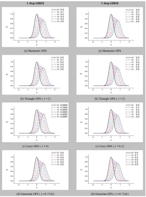
T =1000 ; κ =0.05; U=1.5. (36) The numerical results are shown Fig. 1. In case of zero boundary values and continuous initial value distribution, every GFS gives the same accuracy.

In the calculations in sections 4.2-4.4, the parameters for numerical calculations are as follows:

5 . 0

=

L ; N=40; dx=2L N; dt=0.0005; dt

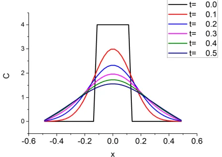
T=1000~16000 ; κ =0.05; U=0. (37) 4.2. Effects of Discontinuous Initial Value Distribution

The boundary and initial conditions for the first example in this section are given by

0 ) , (−Lt =

C , C(+L,t)=0 for t>0, (38)

   _≤ = otherwise 0 4 / 2 ) 0 ,

(x L x L

C , (39)

respectively. The numerical results are shown Fig. 2. Spurious oscillation appears in the results using 2-Step GIRM with harmonic GFS.

The initial condition for the second example is given by

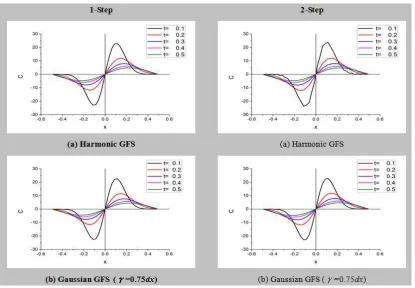
      ≤ < + < ≤ − − = otherwise 0 2 0 ) 2 ( 1 0 2 ) 2 ( 1 ) 0 , ( 2 2 dx x dx x dx dx x

C , (40)

respectively. The numerical results are shown in Fig. 3. Spurious oscillation appears in the results using 2-Step GIRM with harmonic GFS.

4.3. Effects of Non-zero Boundaryl Values

1 ) , (−Lt =

C , C(+L,t)=0 for

t

>

0

, (41) 0

) 0 , (x =

C in −L<x<+L, (42)

respectively. The numerical results are shown in Fig. 4. The results using 1-Step GIRM with Gaussian GFS is not correct. Spurious oscillation appears in the results using 2Step GIRM with Gaussian GFS.

Figure 2. Rectangular initial value distribution

Figure 4. Zero initial value distribution with C(-L,t)=1 and C(+L,t)=0

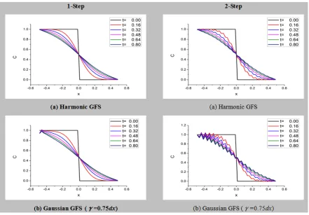
Figure 6. Step-function-like initial value distribution

The boundary and initial conditions for the second example in this section are given by

1 ) , (−Lt =

C , C(+L,t)=1 for t>0, (43) 0

) 0 , (x =

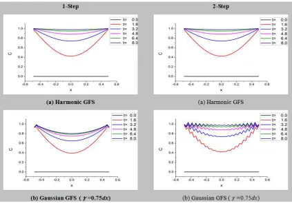
C in −L<x<+L, (44) respectively. The numerical results are shown in Fig. 5. The results using 1-Step GIRM with Gaussian GFS is not correct. Spurious oscillation appears in the results using 2-Step GIRM with Gaussian GFS.

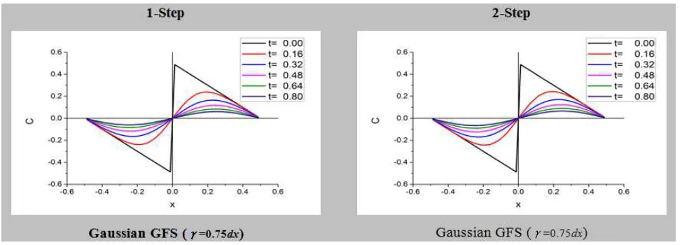
4.4. Simultaneous Effects of Discontinuous Initial Value Distribution and Non-zero Boundary Values

The boundary and initial conditions for example in this section are given by

1 ) , (−Lt =

C , C(+L,t)=0 for t>0, (45)

    

= < =

otherwise 0

0 5 . 0

0 1

) 0 ,

( x

x x

C , (46)

respectively. The numerical results are shown in Fig. 6. The results using 1-Step GIRM with Gaussian GFS is not correct. The spurious oscillation in the results using 2-Step GIRM with harmonic GFS appears because of the discontinuity in the initial value distribution, and that in the results using 2-Step GIRM with Gaussian GFS appears because of the non-zero boundary values.

Table 1. 1-Step GIRM

Continuity of G~ Non-zero boundary _value Discontinuous initial _{value dist.}

0

C Good Good

1

C and _C2 _{Must be much improved Good}

∞

C Must be much improved Good

Table 2. 2-Step GIRM

Continuity of G~ Non-zero _{boundary value} Discontinuous initial value _dist.

0

C Good Must be slightly improved

1

C and _C2 _{Good Good}

∞

C Must be improved Good

4.5. Summary on the Effects of GFSs

would be increased.

5. Remedies for Obtaining Correct

Solutions by GIRM in Case of

Non-zero Boundary Values

5.1. Remedy in Case of Non-zero Bounday Values

In this case, we transform the non-zero bounday value problem into the zero boundary value problem. When the steady state solution C0(x) satisfying

2 0 2 0

dt C d dx dC

U =κ in −L<x<+L, (47)

L g L

C0(− )= ₋ , C0(+L)=g+L (48)

is known, we rewrite C(x,t) as ) , ( ) ( ) ,

(xt C0 x C1 xt

C = + or C1(x,t)=C(x,t)−C0(x). (49) Substituting Eq. (49) into Eqs. (4), (6) and (7), we have

2 1 2 1 1

t C x

C U t C

∂ ∂ = ∂ ∂ + ∂

∂ _κ

in −L<x<+L for t>0, (50)

0 ) , ( 1 −Lt =

C , C1(+L,t)=0 for t>0, (51)

) 0 , ( ) ( ) 0 ,

( 0

1 x f x C x

C = − in −L<x<+L. (52) The non-zero bounday value problem is now transformed into the zero boundary value problem. For example, the boundary and initial values for the transformed problem of the original problem shown in Fig. 5(b) are given by

0 ) , ( 1 −Lt =

C , C1(+L,t)=0 for t>0, (53)

1 ) 0 , ( 1 ) 0 ,

( 0

1 x = −C x =

C in −L<x<+L, (54) respectively. The numerical results are shown in Fig. 7. If

) , ( ) ( ) ,

( 1

0 xt f x C xt

C = − is obtained, C0(x,t) gives the correct solution for the original problem.

For another example, the boundary values and initial value distribution for the transformed problem of the original problem shown in Fig. 6(b) are given by

0 ) , ( 1 −Lt =

C , C1(+L,t)=0 for t>0, (55)

Figure 7. Transformed version of step-function-like initial value distribution

  

  

 

> −

   

 

+ −

= < −

   

 

+ −

=

0 in 0 1 5

. 0

0 x at 0

0 in 1 1 5

. 0

) 0 , ( 1

x L

x

x L

x

x

C , (56)

respectively. The numerical results are shown in Fig. 8. If )

, ( ) ( ) ,

( 1

0 xt f x C xt

C = − is obtained, C0(x,t) gives the correct solution for the original problem.

5.2. Remedies in Case of Discontinuous Initial Value Distribution

In this case, small amount of artificial damping is effective to reduce spurious oscillation [11,12]. Specifically, for example, a numerical damping:

(

)



  

 

+ + −

− + (−1)

) ( ) (

1 )

(

2 2

4 1

4 n

i n i n i n

i C C C

C dx

α

(57)

is added to Ci(n) at every time step n of the time evolution

of (n)

i

C , where α is damping constant. For example, with respect to the problem shown in Fig. 2(a), the numerical results are shown in Fig. 9, where the artificial damping coefficient α =0.000005 is used. The spurious oscillation is elliminated.

Figure 9. Rectangular initial value distribution (Harmonic GFS, 2-Step; α=0.000005)

For example, with respect to the problem shown in Fig. 6(a), the numerical results are shown in Fig. 10, where the artificial damping coefficient α =0.000005 is used. The spurious oscillation is elliminated.

The other method is to use initial filter. If the discontinuity of initial density distribution invites serious errors, it is effective to replace Ci(0)=C(xi,0) with a filtered value such as

(

(0)

)

1 ) 0 ( ) 0 (

1 2

4 1

−

+ + i + i

i C C

C . (58)

Figure 10. Rectangular initial value distribution (Harmonic GFS, 2-Step; α=0.000005)

6. Conclusions

Integral Representation Method (IRM) is developed to Generalized Integral Representation Method (GIRM) and can treat any kinds of problems including nonlinear problems. GIRM uses Generalized Fundamental Solution (GFS) instead of Fundamental Solution (FS). We can use various GFSs for an individual problem. The characteristics of individual GFSs were clarified in the present paper. The continuity of GFS is related to the characteristics of individual GFSs. For example, in one-dimensional case, GFSs with discontinuous and continuous slopes showed quite different property. Furthermore, the degree of continuity had important effects on the property. For simplicity, we discussed one-dimensional advective diffusion problems.

The effects of the continuity of GFS were different between 1-Step and 2-Step GIRMs. Since 1-Step GIRM is impossible for multi-dimensional convective problems, 2-Step GIRM is very important for the problems. When the boundary values were not zero, 1- and 2-Step GIRMs using Gaussian GFS gave unsatisfactory results. 1-Step GIRMs using C1 nd C2 continuous GFSs gave also unsatisfactory results. When the initial value distributions were discontinuous, 2-Step GIRM using GFSs with discontinuous slope gave unsatisfactory results. The remedies to these cases were given in section 5.

References

[1] Wu J.C., Thompson J.F., “Numerical solutions of time-dependent incompressible Navier-Stokes equations using an integro-differential formulations”, Computers & Fluids, (1973), 1, pp. 197-215.

[2] S. J. Uhlman, “An integral equation formulation of the equations of motion of an incompressible fluid”, NUWC-NPT Technical Report 10,086, 15 July, (1992).

[4] H. Isshik, S. Nagata, Y. Imai, “Solution of a diffusion problem in a non-homogeneous flow and diffusion field by the integral representation method (IRM)”, Applied and Computational Mathematics, 3(1), (2014), pp. 15-26. http://article.sciencepublishinggroup.com/pdf/10.11648.j.acm. 20140301.13.pdf

[5] H. Isshiki, Theory and application of the generalized integral representation method (GIRM) in advection diffusion problem, Applied and Computational Mathematics, 3(4), (2014), pp. 137-149.

http://article.sciencepublishinggroup.com/pdf/10.11648.j.acm. 20140304.15.pdf

[6] H. Isshiki, T, Takiya and H. Niizato, Application of Generalized Integral representation (GIRM) Method to Fluid Dynamic Motion of Gas or Particles in Cosmic Space Driven by Gravitational Force, Applied and Computational Mathematics, Special Issue: Integral Representation Method and Its Generalization, (2015), under publicaion. http://www.sciencepublishinggroup.com/journal/archive.aspx? journalid=147&issueid=-1

[7] H. Isshiki, From Integral Representation Method (IRM) to Generalized Integral Representation Method (GIRM), Special Issue: Integral Representation Method and Its Generalization,

(2015), under publicaion.

http://www.sciencepublishinggroup.com/journal/archive.aspx? journalid=147&issueid=-1

[8] Gingold R.A, Monaghan J.J., “Smoothed particle hydrodynamics: theory and application to non-spherical stars,” Mon. Not. R. Astron. Soc., Vol 181, (1977) , pp. 375–89. http://articles.adsabs.harvard.edu/cgi-bin/nph-iarticle_query?1 977MNRAS.181..375G&amp;data_type=PDF_HIGH&amp;w hole_paper=YES&amp;type=PRINTER&amp;filetype=.pdf [9] Lucy L. B., A numerical approach to the testing of the fission

hypothesis, The Astronomical Journal, vol. 82, no. 12 (1977),

pp. 1013-1024.

http://articles.adsabs.harvard.edu/cgi-bin/nph-iarticle_query?1 977AJ...82.1013L&defaultprint=YES&filetype=.pdf [10] Monaghan J. J., Smoothed particle hydrodynamics, Ann.

Reviews Astron. Astrophysics, 30, (1992) , pp. 543-573. [11] H. Isshiki, A method for Reduction of Spurious or Numerical

Oscillations in Integration of Unsteady Boundary Value Problem, AJET, 2, 3, (2014), pp. 190-202. file:///C:/Users/l/Downloads/1360-5725-2-PB%20(2).pdf [12] H. Isshiki, “Improvement of Stability and Accuracy of

Time-Evolution Equation by Implicit Integration”, Asian Journal of Engineering and Technology (AJET), Vol. 2, No. 2

(2014), pp. 1339–160.