FLUID OF HARD DISCS
Mukesh Kumar* and Sanjay Kumar1
Department of Physics B. R. A. Bihar University Muzaffarpur-842001 (India) email: [email protected]; [email protected]
1M.D.D.M. College, Muzaffarpur
(Received, February 1, 2005)
ABSTRACT
In present paper a basic theory has been developed for calculation the leading quantum correction to the thermo dynamic properties of the two-dirnensional fluid hard disc. Theoretical efforts have been made to explain the-structural and thermodynamical properties of two- dimensional fluids. Although a strictly two-dimensional picture has been used in predicting the properties of absorbed film. It is required to study about hard-disc system in framing the theory of two-dimensional fluids. It is quite natural to study model fluids with only hard cores and no inter atomic attractions. The simulation results for RDF of the hard discs for same values of density solution2.
Key Word :- Fluid, hard-disc, quantum correction PACS NOs.: 05.70.Ce, 05.30.ch
INTRODUCTION
This paper is concerned with the estimation of the influence of the quantum effects on the structural and thermodynamic properties of the two - dimensional fluid whose molecules interact via a hard - disc potential. In the high density region, the behaviour of a fluid (liquid or gas) is dominated by the excluded volume effects associated with the hard - cores of its constituents. Therefore it is quite natural to study model fluids with only hard cores and no inter atomic attractions. At present the theoretical studies of liquids use almost invariably some hard - core reference fluid as basis for a perturbation expansion of the equilibrium properties of real fluids1,2. The most widely
used hard core reference fluid in two -dimensional fluid is hard discs. However the hard - disc fluid has not been studied sys-tematically.
Several theoretical and experimental efforts have been made in recent years to understand the structural and thermodynamic properties of two - dimensional fluids. Although, ideally flat systems seldom occur, a strictly two - dimensional picture has been used in predicting the properties of absorbed film. The hard sphere fluid is treated as a reference in framing the theory of three - dimensional dense fluid. In the same way, the hard disc fluid may be treated as a reference for the two dimensional fluid. The study of hard -disc system is essential in framing the theory of two - dimensional fluids.
For classical hard disc fluid, consid-erable progress has been made. The theo-retical3-5 and simulation6 results are available
for equation of state. The simulation results for RDF of the hard discs are also available for some values of density d2. The quantum
effect increases with the decrease of tempera-ture. At lower temperature, many terms are required to account for the quantum effects. In this paper we study the influence of quantum effects on the equilibrium proper-ties of the hard disc fluid. We develop a basic theory for calculating the leading quantum correction to the thermodynamic properties of the two - dimensional fluid of hard disc. The properties are expressed in terms of the RDF of the classical hard discs which is discussed in Sec. 3.
2. Basic theory :
We consider, a quantum mechanical two dimensional system of hard discs with an infinitesimal steep repulsive pair potential defined as
u(r) = r < d
= 0 r > d (1)
where d is the diameter of the hard discs and r denotes two - dimensional distance. The quantity of central importance in con-structing the theory of quantum fluid is the Slater sum. For a two - dimensional fluid, it may be defined as
WN(1, 2, ..., N) = N! 2N < 1, 2, ..., N|~
exp (-HN] | (l, 2, ..., N > (2)
where is the thermal wavelength, = (kT)-1
and N is the Hamiltonian of the system.
N = -( 2/2m) i u i j
2
i 1 N
i 1 N
( , ) (3)
Here u(i,j) is the pair potential between particles
i and j and i2 is the two - dimensional
Laplatian operator. ln this case i denotes the position coordinate ri of particle i.
In the semiclassical limit (i.e. at high temperature limit), we can write9,10
WN = W WNc Nm (4)
where
WNc(1, 2, ..., N) = exp [- u
i 1 N
u(i,j)] (5)
is the Boltzmann factor and WNm is a function
which measures the deviation from the classical behaviour. In the case of two - dimensional fluid,WNm is expressed in terms of modified’
Ursell functions U1m. Thus
WNm(1,2,...,N)=1+
i j N
U
2 m(i, j)+
i j<k N
U3 m(i,j, k)
+ i j k<1
N
U2 m(i, j) U
2
m(k, I) + ... (6)
Thus we obtain the expression for WN
WN(1,2,...,N) WNc(1,2,...,N) [1+ (i,j)
+ (i,j,k)+ (i,j)U2m(k,l)+... (7)
For a system of hard discs, U2m and Um3 have
been evaluated1. U
2
m is given by
Um2(r) = 0(r)+1(r)+..., r > d (8)
where
Here
X = [(2)1/2/(/d)] [r/d–1]
and erfc (X) is the complementary error function.
In quantum satistical mechanics, the chemical potential m can be written as
= -ln [QN+1/QN] (10)
where QN is the partition function defined
as
QN = (1/N!2N)
zz
... WN(1,2,...,N) dri i=1N
(11)
Substituting Eq.(7) in (11), we get
QN = QNc[1 +(1/2)2
z
gNc
(1,2)U2m(1,2) dr1
dr2 +0(2) (12)
where QNc and gN c
(1,2) are, respectively, the canonical partition function and RDF of the classical fluid. Using Eq. (12), Eq. (1) can be written as
=c-(1/2)2
z
[gNc
+1(1,2)-gN c
(1,2)]U2m(1,2)
dr1 dr2 + 0(2) (13)
where
c = -ln[gNc+1/gNc] (14)
c is the classical chemical potential.
Using the relation
2[g
N c
+1(1,2)-gN c
(1,2)=(/
N) [2[
gNc
(1,2)]
=(1/v)(/
) [2
gNc
(1,2)] (15)
We drop the subscript N from now on in
=c-(1/2)*
z
[2g2(1,2)+
gc(1,2)/
]
U2m
(1,2) dr2 +0(2) (16)
Other thermodynamic properties can be obtained from the classical potential. Thus the Helmholtz free energy is given by
A/N = (Ac/N) - (1,2)
z
gc(1,2)U2m
(1,2)
dr2 + 0(2) (17)
and the pressure equation is
P/=(Pc/)-(1,2)
z
gc(1,2)+
gc(1,2)/
]
U2m
(1,2)dr2 + 0 (2) (18)
where Ac and Pc are, respectively, the free
energy and pressure of the classical fluid. Substituting Eq.(8) in Eq. (17), we obtain an expression for the free energy of the hard disc fluid, correct to the first order quantum correction
A/N = (Ac/N) - 2(/d)gc(d) + 0((d)2
(19) where
= (/4) d3
is the packing fraction and gc (d) is the classical
RDF at the contact. Similarly Eqs.(18) and (16) can be evaluated to give
P/=(Pc/)+2(/d)gc(d) +gc(d)/
)] + 0 (d)2 (20)
and
= c+2(/d)2gc(d) +
gc(d)/
)]
The RDF gc(d) can be obtained by
solv-ing the PY integral equation discussed in the following section. Alternately gc (d) can also
be obtained using the pressure equation if the pressure is known. In the two - dimensional classical system of hard - discs, the pressure equation is given by 15
Pc/ = 1 + 2 gc(d) (22)
Then it can be shown that
d( / d) (Ac/N) = d2gc(d) (23)
d( / d) (Pc/) = d2gc(d)+ gc(d)/ )]
(24) and
d( / d) (c) = d2[2gc(d)+ gc(d)/ )]
(25) and one can write Eqs.(17) and (19) in the form
A = Ac + A (26)
P = Pc + AP (27)
µ = µc µ (28)
where
A= d( Ac/ d) (29)
P= d(Pc/ d) (30)
µ= d(µc/ d) (31)
and
= (1/22) (/d) (32)
Thus the leading quantum corrections to the thermodynamic properties of the hard disc fluid can be obtained by replacing the actual diameter d by and effective diameter (d+2-3/2). This is identical to those found
for hard sphere9,16. Recently it is generalised
for hard sphere fluid17.
3. Percus - Yevick integral equation for Radial distribution function of hard - disc fluid:
In this section, we consider the RDF of the two - dimensional fluid of hard - discs.
We employ the Percus- Yevick (PY) integral equation, which can be solved analytically for the hard - disc tluid.
In the PY approximation we have a relation
Y(1,2)+C(1,2)-g(1,2) = 0 (33)
Using the relation
g(1,2) = [1 + f(1,2)] Y(1,2) (34) where
f(1,2) = exp [-u(1,2)] - 1 we have
c(1,2) = f(1,2) Y(1,2) (35)
This equation, when substituted in the Ornstein - Zernicke equation18
g(1,2)-1 = c(1,2) + c(1,3) [g(3,2)-1] dr3
(36) gives the PY - integral equation for g(1,2)
g(1,2) = exp [-u(1,2)] [1 + [1 - exp [u(1,3)} g(1,3) (g(2,3)- 1) dr3 (37)
This gives an expression for Y(1,2)
Y(1,2) = 1 + {1 - exp (u(1,3)} g(1,3)
(g(2,3) - 1)dr3 (38)
The PY-approximation is found to be superior, when the repulsive forces are dominant.
For hard discs of diameter d, we have the condition that
g(r) = 0 r < d (39)
On the other hand the function Y(r) is given by
Y(r) = exp [ . u(r) ] g(r) (40) Which remains continuous at r = d.
d 0.1 0.2 0.3 0.4 0.5 0.55
r/d
1.000 1.136 1.306 1.522 1.802 2.177 2.414
1.048 1.126 1.280 1.470 1.711 2.021 2.210
1.096 1.116 1.254 1.421 1.625 1.876 2.202
1.143 1.106 1.230 1.375 1.544 1.741 1.849
1.191 1.097 1.206 1.330 1.468 1.616 1.691
1.239 1.088 1.184 1.288 1.397 1.502 1.549
1.287 1.079 1.162 1.248 1.330 1.398 1.420
1.334 1.070 1.141 1,210 1.269 1.304 1.306
1.382 1.061 1.121 1.175 1.212 1.220 1.205
1.430 1.053 1.102 1.141 1.160 1.144 1.116
1.478 1.046 1.085 1.110 1.113 1.077 1.040
1.525 1.3038 1.068 1.082 1.070 1.019 0.974
1.573 1.032 1.053 1.056 1.032 0.969 0.919
1.621 1.025 1.038 1.032 0.998 0.927 0.875
1.669 1.019 1.025 1.011 0.969 0.893 0.839
1.717 1.013 1.013 0.992 0.944 0.865 0.814
1.764 1.009 1.003 0.976 0.925 0.846 0.797
1.813 1.004 0.993 0.963 0.910 0.834 0.790
1.860 1.000 .986 0.953 0.900 0.830 0.792
1.908 1.997 0.980 0.946 0.896 0.835 0.805
1.956 0.995 0.977 0.944 0.900 0.852 0.833
2.003 0.994 0.978 0.950 0.916 0.890 0.887
2.051 0.995 0.982 0.962 0.944 0.944 0.960
2.099 0.996 0.986 0.972 0.966 0.986 1.015
2.147 0.997 0.989 0.981 0.984 1.017 1.053
2.195 0.997 0.991 0.989 0.999 1.040 1.079
2.243 0.998 0.994 0.994 1.010 1.054 1.093
2.290 0.998 0.996 0.9999 1.017 1.062 1.098
2.338 0.999 0.998 1.002 1.022 1.065 1.096
2.386 0.999 0.999 1.006 1.025 1.063 1.088
2.434 0.999 1.000 1.O07 1.026 1.059 1.077
2.482 1.000 1.001 1.008 1.026 1.051 1.063
2.530 1.000 1.001 1.009 1.024 1.042 1.048
2.578 1.000 1.001 1.009 1.021 1.U33 1.031
2.673 1.000 1.002 1.007 1.014 1.012 1.001
2.721 1.000 1.001 1.006 1.010 1.002 0.988
2.769 1.00 1.001 1.005 1.006 0.994 0.977
2.817 1.000 1.001 1.003 1.001 0.986 0.969
2.864 1.000 1.001 1.002 0.988 0.980 0.963
2.912 1.000 1.001 1.001 0.996 0.977 0.960
2.960 1.000 1.000 1.000 0.993 0.975 0.960
3.008 1.000 1.000 0.999 0.992 0.975 0.963
3.056 1.000 1.000 0.998 0.992 0.977 0.969
3.103 1.000 1.000 0.998 0.992 0.981 0.977
3.151 1.000 1.000 0.998 0.993 0.985 0.984
3.199 1.000 1.000 0.998 0.994 0.990 0.993
3.247 1.000 1.000 0.998 0.995 0.994 1.000
3.295 1.000 1.000 0.998 0.996 0.999 1.006
3.343 1.000 1.000 0.999 0.998 1.002 1.001
3.390 1.000 1.000 0.999 0.999 1.005 1.014
3.438 1.000 1.000 0.999 1.000 1.007 1.016
3.486 1.000 1.000 0.999 1.000 1.008 I.017
3.534 1.000 1.000 1.000 1.001 1.009 1.016
3.582 1.000 1.000 1.000 1.002 1.009 1.015
3.629 1.000 1.000 1.000 1.002 1.008 1.012
3.677 1.000 1.000 1.000 1.002 1.007 1.010
3.725 1.000 1.000 1.000 1.002 1.006 1.007
3.773 1.000 1.000 1.000 1.002 1.004 1.004
3.820 1.000 1.000 1.000 1.002 1.003 1.001
3.868 1.000 1.000 1.000 1.001 1.001 0.998
3.916 1.000 1.000 1.000 1.001 1.000 0.996
3.964 1.000 1.000 1.000 1.001 0.998 0.994
4.011 1.000 1.000 1.000 1.000 0.997 0.993
C(r) = -Y(r) , r < d
= 0 , r > d (41)
Substituting Eqs.(39) and (41) in Eq.(38) leads to an integral equation for Y(r)
Y(r)=1+ Y(r’)dr’- Y(r’)Y(|r-r’|)dr’|r-r’|>d
r'<d r'<d (42)
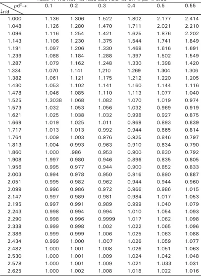
We follows the method of Lado18 to evaluate
Eq.(42) and obtain the values of g(r) for the hard disc fluid over the range of density d2.
The values of g(r) of the hard dise fluid are reported in tables 1 and 2 for 0. 10 d2 0.55 and 0.60 d2 0.75, respectively.
d 0.60 0.65 0.70 0.75
r/d
1.000 2.697 3.039 3.457 3.978
1.053 2.398 2.644 2.931 3.269
1.107 2.127 2.292 2.470 2.661
1.161 1.885 1.983 2.076 2.055
1.215 1.672 1.716 1.742 1.740
1.269 1.485 1.488 1.465 1.405
1.323 1.324 1.295 1.238 1.143
1.377 1.187 1.135 1.056 0.942
1.430 1.071 1.005 0.913 0.792
1.484 0.975 0.900 0.804 0.687
1.538 0.897 0.820 0.726 0.617
1.591 0.837 0.761 0.673 0.579
1.646 0.792 0.720 0.643 0.566
1.699 0.763 0.698 0.633 0.575
1.753 0.747 0.692 0.612 0.604
1.807 0.745 0.702 0.668 0.651
1.861 0.757 0.728 . 0.713 0.718
1.915 0.786 0.774 0.780 0.808
1.969 0.838 0.847 0878 0.937
2.022 0.938 0.980 1.053 1.65
2.076 1.032 1.100 1.202 1.342
2.130 1.094 1.171 1.276 1.409
2.184 1.129 1.202 1.295 1.400
2.238 1.143 1.206 2.278 1.344
2.291 1.141 1.190 1.234 1.262
2.345 1.128 1.160 1.179 1.170
2.399 1.108 1.122 1.117 1.078
2.453 1.083 1.081 1.056 0.995
2.507 1.055 1.040 1.000 0.925
2.560 1.028 1.003 0.952 0.871
2.614 1.033 0.970 0.914 0.835
2.668 0.981 0.943 0.887 0.815
2.722 0.963 0.923 0.870 0.811
2.776 0.909 0.911 0.866 0.811
2.883 0.937 0.910 0.887 0.880
2.937 0.940 0.920 0.911 0.925
2.991 0.947 0.939 0.944 0.978
3.044 0.960 0.962 0.984 1.036
3.099 0.976 0.989 1.022 1.087
3.152 0.991 1.012 1.054 1.123
3.206 1.006 1.031 1.076 1.140
3.260 1.017 1.044 1.086 1.138
3.314 1.025 1.051 1.086 1.122
3.368 1.030 1.052 1.078 1.095
3.421 1.030 1.048 1.064 1.062
3.475 1.029 1.041 1.045 1.027
3.529 1.025 1.031 1.025 0.993
3.583 1.020 1.020 1.005 0.964
3.637 1.014 1.008 0.987 0.941
3.690 1.007 0.997 0.972 0.926
3.744 1.001 0.988 0.960 0.919
3.798 0.995 0.980 0.960 0.919
3.852 0.991 0.975 0.952 0.927
3.90G 0.987 0.973 0.954 0.941
3.959 0.985 0.973 0.960 0.960
4.013 0.985 0.976 0.970 0.981
Table 3. Equation of state P / for hard disc fluid
From Eq.(43) From Eq.(44)
0.10 1.1785 1.1787
0.20 1.4104 1.4119
0.30 1.7170 1.7237
0.40 2.1320 2.1528
0.50 2.7094 2.7649
0.55 3.0858 3.1733
0.60 3.5421 3.6783
0.65 4.1027 4.3128
0.70 4.8012 5.1243
The results are demonstrated in Table 3. We have also calculated the equation of state us-ing the expression
Pc/ = (1 + 0.1262) / (1 - )2 (44)
The argument is good for d2 0.50.
Descripancy inereases with increases of density. One is expected to improve the results by using the PY2 approximation. However it is time consuming, so it is not attempted here.
4. RESULT AND DISCUSSION
A method has been developed for calculating the leading quantum correction to the thermodynamical properties and classical RDF of the two-dimensional fluid of hard discs. This gives good results at high tempera-ture where quantum effects are small. The estimation of the influence of the quantum effects on the structural and thermodynamical properties of the two-dimensional fluid
liquids are almost invariably some hard core reference fluid as basis for a perturbation expan-sion of the equilibrium properties of real flu-ids1,2.
The quantum effects increases with the decreases of temperature. At lower tempera-ture, many terms are required to account for quantum for quantum effects. In the semiclassical limit (i.e. at high temperature) where quantum limit (i.e. at high temperature) whence quantum effects are small and treated as a correction to the classical behaviour, the usual way is to expand the properties about this classical vafues.
ACKNOWLEDGEMENT
The author is thankful to Prof S. K. Sinha, Deptt. of Physics, L. S. College, Muzaffarpur for providing supported suggestion. Further author is also thankful to Dr. C.S.Rai, Deptt. of Physics, R.D.S. College, Muzaffarpur for his encouragement.
1. Hansen, J. P. and Mc Donald, I. R., Theory of Simple Liquids (Acad. Press New York) (1976).
2. Mc Quarrie D.A., Statistical Mechanics (Harper and Row, New York) (1976). 3. Reiss, H., Frisch, H. L. and Lebowitz J. L., J. Chem. Phys. 31, 369 (1959). 4. Henderson, D., Mol. Phys., 30, 971
(1975).
Mol. Phys. 31, 301 (1977).
5. Kratky, K.W., Physica 85A, 607 (1976).
J. Chem, Phys., 69, 2251 (1978). 6. Erpenbeck, J. J. and Lubon, M., Phys.
Rev. A32, 1403 (1985).
7. Chae, D. C., Ree, E. W. and Ree, J.,
REFERENCES
J. Chem. Phys.,50, 1981 (1969). 8. Wood, W. W., J. Chem. Phys.,52,
729 (1970).
9. Hemmer, P.C., Phys. Lett., A 27, 277 (1968).
10. Jancovici, B., Phys. Rev.,178, 295 (1969).
11. Sinha, S. K. and Singh, Y., Mol. Phys.,
44, 877 (1981).
12. Ram J. Sainger, Y.S. and Singh, Y., Mol. Phys., 45, 1141 (1982). 13. Sainger, Y.S., Sinha, S. K. and Singh,
Y., J. Chem Phys., 79, 5088 (1983). 14. Singh, Y. and Sinha, S.K., Phys. Rept.,
15. Helfand, E., Frisch, H. L. and Lebowitz J.L., J. Chem. Phys.,34, 1037 (1961). 16. Gibson, W. G., Mol. Phys., 30, 1, 13
(1975).
17. Sinha, S.K., Mol. Phys.,71, 135 (1990). 18. Ornstein, L. S. and Zernike, F., Proc. Acad. Soc. Amst. 17, 793 (1914). 19. Lado F., J. Chem. Phys., 49, 3092
(1981).
20. Singh, T.P., Sinha, J.P. and Sinha, S.K., Pramana J. Phys., 31, 289 (1988). 21. Dey, T.K., Karki, S.S. and Sinha, S.K.,
Indian J. Phys., 78, 751 (2004). 22. Maeso, M.J. and Solana, J.R., J. Chem.
Phys.,101, 9864 (1994).