Published online October 30, 2013 (http://www.sciencepublishinggroup.com/j/hyd) doi: 10.11648/j.hyd.20130102.11
Finite element analysis of tidal currents over the red sea
Samir Abohadima
1, Ahmed Rakha
21
Cairo University, Faculty of Engineering, Dept, of Math, and Eng, Physics
2
Cairo University, Faculty of Engineering, Dept, of Irrigation and Hydraulics
Email address:
[email protected] (S. Abohadima)
To cite this article:
Samir Abohadima, Karim Ahmed Rakha. Finite Element Analysis of Tidal Currents over the Red Sea. Hydrology.
Vol. 1, No. 2, 2013, pp. 12-17. doi: 10.11648/j.hyd.20130102.11
Abstract:
Hydrodynamic models represent the core of any simulation for water quality, siltation, and morphology studies. In this study a finite element model was setup for the Red Sea to predict the tidal currents and tidal water level variations. The boundary for the model is located at the Straits of Bab-al-Mandeb. The model was simulated using two dimensional depth averaged model with an element size varying from 15 km to less than 1 km. The model was shown to provide good results for the water level variations at many stations in the Red Sea.Keywords:
Finite Element, Red Sea, Unstructured Grid, Tidal Currents and Tides1. Introduction
Hydrodynamic models (HD) represent the core of any simulation for water quality, siltation, and morphology studies. HD models vary from fully three dimensional 3D to simpler one dimensional 1D model. Such models may differ in the choice of the numerical grid, the discretization method, the time difference scheme, the solution technique, and the treatment of boundary conditions. Finite difference models using Cartesian grids require the application of several nested models in order to model a certain area with a fine grid. Finite element models, have the advantage that an unstructured grid can be used thus providing fine grid resolution in the areas of interest only.
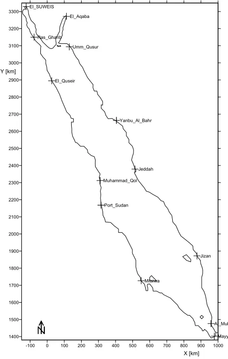
The Red Sea is a basin of the Indian Ocean between Africa and Asia , Fig. 1. The Red Sea is located between 12ºN and 30ºN Lat. And 32ºE and 44ºE Long. The Red Sea is one of the world’s most enticing natural seascape environments that began to develop 20-30 million years ago when the plates of East Africa and Arabia stretched-out until they broke apart.
The Red Sea contains extensive reef systems due to large depths and efficient water circulation patterns. The Red Sea water mass exchanges water with the Arabian Sea, Indian Ocean via the Gulf of Aden. These physical factors reduce the effect of increased salinity caused by evaporation and cold water in the north and relatively hot water in the south.
Reference [1] suggests that there are actually three amphidromic points; one off the coast of Port Sudan, another
off the coast of Assab and yet another between Tor and Ashrafi Island.
The Red Sea is quite narrow and deep but elongated, because of its tectonic origins. There are shallow shelves in the southern end on either side of the Straits connecting the Red sea to the Gulf of Aden. There is no significant contact with the Mediterranean except through the narrow Suez Canal. Because of the highly restricted connection through the Straits of Bab-al-Mandeb to the Gulf of Aden and the Arabian Sea, the tides in the Red Sea are rather low. Tidal ranges in meter as presented by [2] and [3].
There is some amplification of tides on the shallow shelves in the southern Red Sea near the Straits of Bab-al-Mandeb. As presented by [2] the tidal range varies from zero (near amphidromic points) to 2.1 m (Suez). The maximum recorded water level was 2.1 m at Suez port during the month of January. The tides are also predominantly semidiurnal all over the Red Sea.
investigate the gravitational and dynamical adjustment of the Red Sea outflow where it is injected into the open ocean in the western Gulf of Aden. Reference [8] Studies the tidal currents and water level variations along the Red sea. Reference [9] solved combined wind and density-driven circulation in enclosed seas with variable Coriolis parameter assuming the basin is elliptic shape. Reference [10] Calculates the water circulation numerically inside the A red sea due to winds, but did not include the tidal currents effects. In this study, we simulate the water circulations and surface variations due to tidal variations and Coriolis forces overall the red sea numerically using finite element method.
2. Model Description
In this study, the RMA-10 model was set up for the Red Sea. The hydrodynamic model is a three dimensional finite element HD model as in [11] capable of simulating steady and unsteady currents. The RMA model uses an unstructured grid making it suitable for generating finer grids in the areas of interest.
3. Governing Equations
The full nonlinear Navier Stokes equation for three dimensions together with the continuity equations are used to describe the flow. The equations are modified to make the assumption of hydrostatic pressure and transformed to a constant grid to facilitate automatic solution of the free surface problem. Salinity, temperature and suspended sediment are simulated using the advection diffusion equation coupled to density through equations of state. For the Red Sea model we used the two dimensional depth average approximation. The full nonlinear set of equations may be integrated over transformed vertical dimension with
the assumption that horizontal velocity components u and v
are independent of elevation z. Under these conditions all
derivatives with respect to z are eliminated. The governing
equations may thus be written as: Momentum Equation
ρ(b-a) (h∂ u
∂t + hu
∂u
∂x + hv
∂u
∂y -
1
ρ∂∂x (εxx h
∂u
∂x)
- 1
ρ∂∂y (εxy h
∂u
∂y ) + gh (
∂a
∂x +
∂h
∂x))
- (b-a) gh2
2
∂ρ
∂x - (b-a) h Γx = 0 (1)
ρ(b-a) ((h∂ v
∂t + hu
∂v
∂x + hv
∂v
∂y -
h
ρ∂∂x (εyx
∂v
∂x)
- h
ρ∂∂y (εyy
∂v
∂y ) + gh (
∂a
∂y +
∂h
∂y))
- (b-a) gh2
2
∂ρ
∂y - (b-a) h Γy = 0 (2)
Continuity Equation
(h∂ u
∂x +
∂v
∂y) + u
∂h
∂x + v
∂h
∂y +
∂h
∂t = 0 (3)
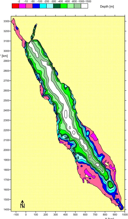
4. Bathymetric Data
The bathymetric data was taken from the Naval
Oceanographic office in the USA
(http://www.ngdc.noaa.gov/ngdc.html). The grid spacing for the bathymetric data was 2 minutes and for the topographic data was 0.5 minutes. Shoreline data was also obtained from the same source. The data is in Geographic coordinates (latitude and longitude). Fig. 2 provides a relief map that includes the topographic data generated from this data.
The bathymetric data and shoreline data was converted into Universal Transverse Mercator (UTM) coordinates for Zone 37. The UTM data was used in the RMA model.
-100 0 100 200 300 400 500 600 700 800 900 1000 1400
1500 1600 1700 1800 1900 2000 2100 2200 2300 2400 2500 2600 2700 2800 2900 3000 3100 3200 3300
Al_Mukha Mitsiwa
Jizan Port_Sudan
Muhammad_Qol Jeddah Yanbu_Al_Bahr El_Quseir
Umm_Qusur Ras_Gharib
El_Aqaba El_SUWEIS
Mayyun
X [km] Y [km]
Figure 1. Map of the Red Sea.
5. Model Setup
and Gulf of Aquaba. The elements were chosen to be longer along the Red Sea axis since the flow is expected to vary less rapidly along the longer axis. The actual grid resolution will be half the above figure since nodes are placed in the center of sides of the different elements. Both triangular and quadrilateral elements were used.
The tidal constituents at the Mayyun Port 12°39'N, 43°24'E Republic of Yemen were used to generate tidal water levels for the boundary condition at the entrance of the Red Sea. The water level was assumed to be constant along the boundary line at the entrance of the red sea. This will be a reasonable assumption due to the narrow nature of the entrance. There is no significant contact with the Mediterranean due to the Suez Canal as in [2]. Accordingly the input boundary condition is only restricted at one entry at Bab El Mandab.
The Smagorinsky turbulence model was used and a manning friction factor of 0.02. This manning coefficient was obtained by calibrating the model for different stations as explained later. A time step of 0.2 hours was used in all the simulations.
-100 0 100 200 300 400 500 600 700 800 900 1000 1400
1500 1600 1700 1800 1900 2000 2100 2200 2300 2400 2500 2600 2700 2800 2900 3000 3100 3200 3300
-1500 -1000 -800 -600 -400 -300 -200 -100 -50 -10 -2
X [km] Y [km]
Depth [m]
Figure 2. Bathymetric Map of the Red Sea.
-100 0 100 200 300 400 500 600 700 800 900 1000 1400
1500 1600 1700 1800 1900 2000 2100 2200 2300 2400 2500 2600 2700 2800 2900 3000 3100 3200 3300
X [km] Y [km]
Figure 3. Computational Grid Covering the Red Sea.
6. Model Calibration/Validation
The RMA Model was calibrated/validated using tidal water level data obtained from a tidal model TIDECALC. The TIDECALC software, is a version of the tidal prediction program developed by the UK's Hydrographic Office for publication in the Admiralty Tide Tables. Fig. 6 provides the location of the stations that were used to validate the RMA Model and Table 1 provides the location for these stations.
Table 1. Stations used to Validate the RMA Red Sea Model
Station
No. Station Name Longitude Latitude
1 Suez (Egypt) 32°33' 29°56'
2 Ras Gharib (Egypt) 33°07' 28°21'
3 El Quoseir (Egypt) 34°16' 26°06'
4 Port Sudan (Sudan) 37°14' 19°36'
5 Mohamed Qoul (Sudan) 37°10' 20°54'
6 Missawa (Eriteria) 39°28' 15°37'
7 Al Aquaba (Jordan) 35°00' 29°31'
8 Umm Qusur (Saudi Arabia) 35°14' 27°55'
9 Yanbu El Bahr (Saudi Arabia) 38°04' 24°05'
10 Jeddah (Saudi Arabia) 39°08' 21°31'
11 Jizan (Saudi Arabia) 42°32' 16°54'
The verification presents the water level calculated by the RMA model together with the water level predicted by TIDECALC at the same location during the same time interval (30 days considered). At each location an error analysis was performed.
Figs. 6 to 9 show sample plots for the RMA model results at some of these stations. A period of 30 days is provided in these figures representing two spring neap cycles. It can be seen that the model predicts the tidal water levels well.
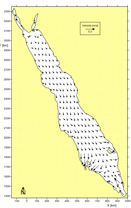
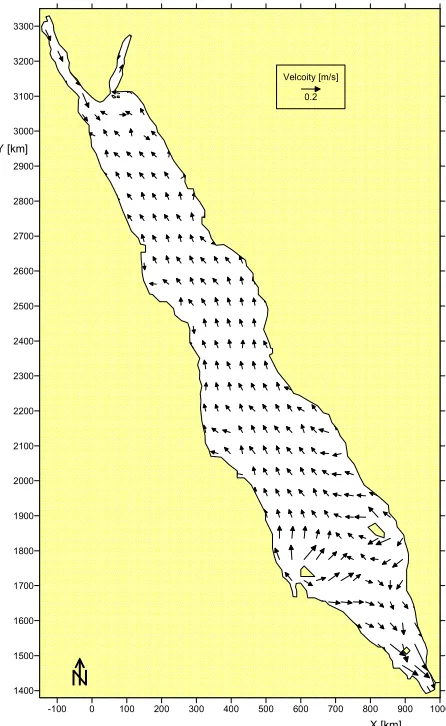
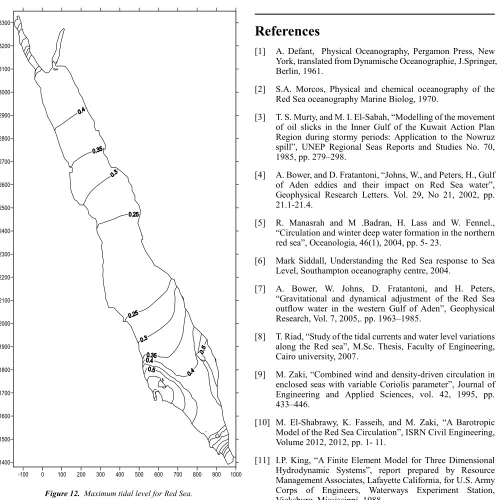
Figs. 10 to 11 provide sample plots for the tidal currents at a certain instant. Fig. 12 provides the maximum tidal currents predicted over a 30 day period. It can be seen that for most of the Red Sea, the tidal currents are below 0.4 m/s. Fig.13 provides the maximum tidal levels predicted over a 30 day period. It can be seen that predicted levels are in good agreement with values given by [3].
0 0.5 1 1.5 2 2.5
0 48 96 144 192 240 288 336 384 432 480 528 576 624 672 720 768 816 864 912 960
W
a
t
e
r
L
e
v
e
l
(m
)
Time from Jan. 1, 2012 (hr)
Figure 4. Tidal data used at entrance of Red Sea.
0.0 0.2 0.4 0.6 0.8 1.0 1.2 1.4
96 144 192 240 288 336 384 432 480 528 576 624
W
a
te
r
L
e
v
e
l
(m
)
Time from Jan. 1, 2012 (hr)
RMA TideWizard
Figure 5. Sample of hydrodynamic Model Calibration at Gizan
0 0.2 0.4 0.6 0.8 1 1.2 1.4
96 144 192 240 288 336 384 432 480 528 576 624
W
a
te
r
L
e
v
e
l
(m
)
Time from Jan. 1, 2012 (hr)
RMA TideWizard
Figure 6. Sample of hydrodynamic Model Calibration at Jeddah.
0 0.2 0.4 0.6 0.8 1 1.2 1.4
96 144 192 240 288 336 384 432 480 528 576 624
W
a
te
r
L
e
v
e
l
(m
)
Time from Jan. 1, 2012 (hr)
RMA TideWizard
Figure 7. Sample of hydrodynamic Model Calibration at Quseir.
0 0.2 0.4 0.6 0.8 1 1.2 1.4
96 144 192 240 288 336 384 432 480 528 576 624
W
a
te
r
L
e
v
e
l
(m
)
Time from Jan. 1, 2012 (hr)
RMA TideWizard
Figure 8. Sample of hydrodynamic Model Calibration at Port Sudan.
-100 0 100 200 300 400 500 600 700 800 900 1000 1400
1500 1600 1700 1800 1900 2000 2100 2200 2300 2400 2500 2600 2700 2800 2900 3000 3100 3200 3300
Velcoity [m/s] 0.2
X [km] Y [km]
-100 0 100 200 300 400 500 600 700 800 900 1000 1400
1500 1600 1700 1800 1900 2000 2100 2200 2300 2400 2500 2600 2700 2800 2900 3000 3100 3200 3300
Velcoity [m/s] 0.2
X [km] Y [km]
Figure 10. Hydrodynamic Red Sea model results on Feb. 11, 2012 (hour 16.5, flood conditions).
-100 0 100 200 300 400 500 600 700 800 900 1000 1400
1500 1600 1700 1800 1900 2000 2100 2200 2300 2400 2500 2600 2700 2800 2900 3000 3100 3200 3300
0 0.01 0.02 0.05 0.1 0.15 0.2 0.25 0.3 0.35 0.4
X [km] Y [km]
Velocity [m/s]
Figure 11. Maximum tidal currents for Red Sea.
7. Conclusions
In this study the RMA-10 finite element hydrodynamic model was setup to model the tidal currents and water level variations for the Red Sea. The model was run in two dimensional mode with the boundary located at Bab El Mandab. The element size varied from 15 km to less than 1.0 km. The model was validated using a tide prediction model that is based on measurements for the water level. The model results showed that the model is capable of predicting the tidal water level variations well. The model showed that the tidal currents in the Red Sea are mostly below 0.4 m/s except near the Red Sea entrance. This model will be useful for generating boundary conditions for local models with the Red Sea.
Nomenclature
x, y are the horizontal Cartesian coordinate system
ρ is the water density
g is the acceleration due to gravity
p is the water pressure
εxx, εxy and εyy are the turbulent eddy coefficients;
Γ is the external tractions that operate on the boundaries or
on the interior;
Dx, Dx are the eddy diffusion coefficients for salinity; θs is the source/sink for salinity;
b is the fixed vertical location to which the water surface
will be transformed;
a is the elevation of the bottom relative to the same vertical datum;
-100 0 100 200 300 400 500 600 700 800 900 1000 1400
1500 1600 1700 1800 1900 2000 2100 2200 2300 2400 2500 2600 2700 2800 2900 3000 3100 3200 3300
Figure 12. Maximum tidal level for Red Sea.
References
[1] A. Defant, Physical Oceanography, Pergamon Press, New York, translated from Dynamische Oceanographie, J.Springer, Berlin, 1961.
[2] S.A. Morcos, Physical and chemical oceanography of the Red Sea oceanography Marine Biolog, 1970.
[3] T. S. Murty, and M. I. El-Sabah, “Modelling of the movement of oil slicks in the Inner Gulf of the Kuwait Action Plan Region during stormy periods: Application to the Nowruz spill”, UNEP Regional Seas Reports and Studies No. 70, 1985, pp. 279–298.
[4] A. Bower, and D. Fratantoni, “Johns, W., and Peters, H., Gulf of Aden eddies and their impact on Red Sea water”, Geophysical Research Letters. Vol. 29, No 21, 2002, pp. 21.1-21.4.
[5] R. Manasrah and M .Badran, H. Lass and W. Fennel., “Circulation and winter deep water formation in the northern red sea”, Oceanologia, 46(1), 2004, pp. 5- 23.
[6] Mark Siddall, Understanding the Red Sea response to Sea Level, Southampton oceanography centre, 2004.
[7] A. Bower, W. Johns, D. Fratantoni, and H. Peters,
“Gravitational and dynamical adjustment of the Red Sea outflow water in the western Gulf of Aden”, Geophysical Research, Vol. 7, 2005,. pp. 1963–1985.
[8] T. Riad, “Study of the tidal currents and water level variations along the Red sea”, M.Sc. Thesis, Faculty of Engineering, Cairo university, 2007.
[9] M. Zaki, “Combined wind and density-driven circulation in
enclosed seas with variable Coriolis parameter”, Journal of Engineering and Applied Sciences, vol. 42, 1995, pp. 433–446.
[10] M. El-Shabrawy, K. Fasseih, and M. Zaki, “A Barotropic Model of the Red Sea Circulation”, ISRN Civil Engineering, Volume 2012, 2012, pp. 1- 11.