Quantum Set Intersection and its Application to Associative Memory
Tamer Salman [email protected]
Yoram Baram [email protected]
Department of Computer Science Technion - Israel Institute of Technology Haifa, 32000, Israel
Editor:Manfred Opper
Abstract
We describe a quantum algorithm for computing the intersection of two sets and its application to associative memory. The algorithm is based on a modification of Grover’s quantum search algorithm (Grover, 1996). We present algorithms for pattern retrieval, pattern completion, and pattern correction. We show that the quantum associative memory can store an exponential number of memories and retrieve them in sub-exponential time. We prove that this model has advantages over known classical associative memories as well as previously proposed quantum models.
Keywords: associative memory, pattern completion, pattern correction, quantum computation, quantum search
1. Introduction
The introduction of Shor’s algorithm for factoring numbers in polynomial time (Shor, 1994) has demonstrated the ability of quantum computation to solve certain problems more efficiently than classical computers. This perception was ratified two years later, when Grover (1996) introduced a sub-exponential algorithm for quantum searching a database.
The field of quantum computation is based on the combination of computation theory and quan-tum mechanics. Computation theory concerns the design of computational models and the study of their time and space complexities. Quantum mechanics, on the other hand, concerns the study of systems governed by the rules of quantum physics. The combination of the two fields addresses the nature of computation in the physical world. However, there is still no efficient reduction of quantum mechanical behavior to classical computation.
Quantum mechanics is a conceptual framework that mathematically describes physical sys-tems. It is based on four postulates, known as the postulates of quantum mechanics (Nielsen and Chuang, 2000), which provide a connection between the physical world and mathematical formal-ism. Through these postulates, it is possible to better understand the nature of physical computation and what can be physically computed.
Next, we introduce the basic building blocks of quantum computation. The reader is referred to Nielsen and Chuang (2000) for a detailed introduction.
1.1 States and Qubits
The basic entity of classical computation is the classical bit. Each classical bit can have one of two values, 0 and 1. The state of any finite physical system that can be found in a finite number of states can be described by a string of bits. A string ofnbits represents one of 2npossible states of a system enumerated 0, ..., 2n−1.
In quantum computation, the basic entity is called a qubit (quantum bit). The qubit can have the analogue values|0iand|1i, known as the computational basis states, where|·iis the Dirac notation. Yet, the qubit can also have any other value that is a linear combination of|0iand|1i:
|Ψi=α|0i+β|1i
whereαandβare any complex numbers (called the amplitudes of the basis states 0 and 1, respec-tively), such that|α|2+|β|2=1. Consequently, the qubit can be in any one of an infinite number of states described by unit vectors in a 2-dimensional complex vector space. The unary representation of a qubit can be given as a vector of two values
|Ψi=
α β
.
Analogously to the classical bit string, qubit strings (or quregisters) describe the state of a sys-tem. A two qubit system comprising two qubits|ai=α|0i+β|1iand|bi=γ|0i+δ|1iis described by the tensor product of the two qubits|a,bi ≡ |ai ⊗ |bi=αγ|00i+αδ|01i+βγ|10i+βδ|11i.
1.2 Measurement
The measurement of a qubit reveals only one of two possible outcomes. The value ofαandβcannot be extracted from the measurement of a qubit. Instead, when measuring the qubitα|0i+β|1iin the computational basis, the result can be either 0 or 1 with probabilities|α|2and|β|2respectively. For example, the state
1
√
2|0i+ 1
√
2|1i
, when measured, yields any of the two results 0 or 1 with probability 1/2. The measurement operation is not reversible and, once made, the qubit no longer exists in its state before the measurement. Measurements can be performed in different bases. For example, measuring the qubitα|0i+β|1i in the Hadamard basis defined by the two basis states |+i ≡√1
2|0i+ 1
√
2|1i
and|−i ≡
1
√
2|0i − 1
√
2|1i
gives|+i with probability (α+2β)2 and|−i with probability (α−β)
2
2 , sinceα|0i+β|1i= α+β
√
2 |+i+ α−β
√
2 |−i.
Ann-qubit system can be either measured completely or partially. When measured partially, the unmeasured subsystem can retain quantum superposition and further quantum manipulations can be performed upon it. However, any measurement can be delayed to the end of the computation process.
1.3 Operators
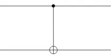
Figure 1: The 2-qubit Controlled-Not (CNOT) quantum gate.
Figure 2: The 3-qubit Toffoli quantum gate.
of the system state. A unitary operator satisfiesUU†=I, whereU†is the conjugate transpose ofU (transpose the matrixU then substitute the conjugate complex of each element in the matrix).
Quantum operators can be implemented using quantum gates, which are the analogue of the classical gates that compose classical electrical circuits. In this analogy, the wires of a circuit carry the information on the system’s state, while the quantum gates manipulate their contents to different states. For example, the Hadamard operator
H= √1
2
1 1 1 −1
transforms a qubit in the state|0iinto the state|+iand the state|1iinto the state|−i.
Operators can also be quantum gates operating on multiple qubits. Ann-qubit quantum oper-ator hasninputs andnoutputs. For example, the 2-qubit controlled-not (CNOT) gate depicted in Figure 1, flips the target (second) qubit if the control qubit (first) has value |1iand leaves it un-changed if the control qubit has the value|0i. Specifically, the CNOT gate performs the following transformations on the four computational basis states:|00i → |00i,|01i → |01i,|10i → |11i, and |11i → |10i. It can be described as a unitary matrix operating on the unary representation of the state as follows:
CNOT =
1 0 0 0 0 1 0 0 0 0 0 1 0 0 1 0
.
Another gate is the 3-qubit controlled-controlled-not gate also known as the Toffoli gate depicted in Figure 2, which flips the target (third) qubit if the two control bits (first and second) both have the values|1iand leaves it unchanged otherwise.
The Hadamard operator can also be seen as operating onn-qubits by the tensor product ofn single qubit Hadamard operators. Each qubit is then transformed according to the single qubit Hadamard transform, that is,
Figure 3: A classical reversible Oracle.
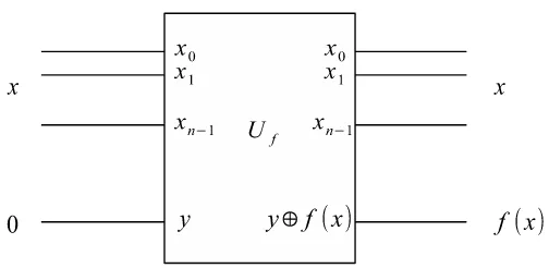
Figure 4: A quantum Oracle.
1.4 Quantum Parallelism and Interference
Consider an oracle of an n-dimensional function f implemented by a classical circuit, which, for every inputx, producesf(x)at the output. The oracle can be made reversible by adding an additional bit to the input, initialized by 0, and letting the output bex,0⊕f(x)as depicted in Figure 3, where ⊕is the addition modulo 2. Initializing the additional bit with 1 produced f(x)at the output.
A quantum oracle is a reversible oracle that accepts a superposition of inputs and produces a superposition of outputs as depicted in Figure 4. When the additional qubit is initialized by|0i, the oracle performs the following transformation:|xi|0i → |xi|0⊕f(x)i. When the additional qubit is initialized by|−ithe oracle is called a quantum phase oracle that gives f(x)in the phase of the state |xias follows:|xi|−i →(−1)f(x)|xi|−i.
1
√
2n∑i=0
2 |ii. The superposition will be maintained through the quantum circuit and the result-ing output would be √1
2n∑
2n
i=0|ii|f(i)i. This can be computed as follows: Uf⊗n+1 H⊗n⊗I|0i⊗n|0i=U⊗f n+1√1
2n 2n
∑
i=0
|ii|0i=√1 2n
2n
∑
i=0
|ii|f(i)i.
Although this computes f for all values ofisimultaneously there is no immediate way of seeing them all together, because once the output state is measured, only one value of f(i) is revealed and the rest vanish. However, further quantum computation allows the different values to interfere together and reveal some information concerning the function f.
It has been shown (Deutsch, 1985; Deutsch and Jozsa, 1992; Simon, 1994) that the revealed information can be considerably more than what classical computation would achieve after one query of the circuit that implements the function f. Deutsch and Jozsa (1992) showed that if a binaryn-dimensional function is guaranteed to be either constant or balanced, then determination can be done using only one query to a quantum oracle implementing it, while a classical solution would require an exponential number of queries. Another example of the advantage of quantum algorithms over classical ones was presented by Simon (1994), in which a function is known to have the property that there exists somes∈ {0,1}nfor which for allx,y∈ {0,1}nit hold that f(x) = f(y)
if and only ifx=yorx⊕y=s. Simon (1994) proved that using quantum computations,scan be found exponentially faster than with any classical algorithm, including probabilistic algorithms.
1.5 Solving Problems using Quantum Computation
According to the above definitions of a system state, measurement, and operators, a quantum com-puter drives the dynamics of the quantum system through operators that change its state and mea-sures the final state to reveal classical information. In the general case, one might think of the process of quantum computation as a multi-phase procedure, which performs some classical compu-tation on the data at hand, creates a quantum state describing the system, drives it through quantum operators, which might depend on the data, to the target state, measures the outcome, and performs some more classical computation to receive a result.
Consequently, we can describe a schematic process for solving problems using quantum com-putation as follows:
A general solution scheme using quantum computations Given:
Classical input data
1. Preliminary classical computation of the input 2. Create initial quantum state
3. Apply quantum circuit to the initial quantum state 4. Measure the resulting state
5. Apply classical computation to the measured state
1.6 Grover’s Quantum Search Algorithm
The algorithm performs a series ofO(√N)unitary operations on the superposition of all basis states that amplify the solution states causing the probability of measuring one of the solutions at the end of the computation to be close to 1.
Suppose that the search problem has a setX ofr solutions and that we own an oracle function fX that identifies the solutionx∈Xaccording to the following:
fX(x) =
1, x∈X 0, x∈/X.
Any classical algorithm that attempts to find the solution clearly needs to query the oracleN times in the worst case. Grover’s algorithm shows that we can find the solution with the help of the oracle by querying it onlyO(√N)times.
The quantum phase oracle of the function fX flips (rotates byπ) the amplitude of the states of X, while leaving all other states unchanged. This is done by the operatorIX =I−2∑x∈X|xihx|. In matrix formulation,IX is similar to the identity matrixIexcept it has−1 on thexth elements of the diagonal.
Grover’s algorithm starts with the superposition of all basis states created by applying the Hadamard operator on the zero state, H⊗n|0i⊗n (shortened by H|0i), and goes about perform-ing multiple iterations, in which each iteration consists of applyperform-ing the phase oracle followed by the operatorHI0H, whereI0flips the phase of the state|0i⊗n. Grover’s iterator is thus defined as
Q=−HI0HIX (1)
where the sign ”−” stands for the global phase flip that has no physical meaning and is performed only for analytical convenience.
The operator in Equation 1 can be viewed in the space defined by the two basis states
|l1i=√1
ri
∑
∈X|iiand
|l2i=√ 1
N−ri
∑
∈/X|ii as the rotation
1−2Nr 2 √
r(N−r)
N
−2 √
r(N−r)
N 1−
2r N
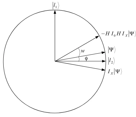
which is depicted in Figure 5, where the rotation angle is
w=arccos
1− 2r
N−r
.
The initial state has an angle
φ=arctan
r
r
N−r
Figure 5: The effect of Grover’s rotation on the state|Ψi.
with|l2i, and after some analysis one can find that applying the operatorT times starting from the initial state yields a solution state with a maximal probability that is very close to 1 upon measure-ment when
T =
$
π 4
r
N r
%
=O
r
N r
!
.
The algorithm performs O
q
N r
iterations, where r=|X|is the number of marked states. Additional improvements were made by Boyer et al. (1996) and Brassard et al. (1998) coping with an unknown number of marked states in complexityO
q
N r
. Biham et al. (1999) introduced a third improvement that outputs a marked state when initiated with a state of an arbitrary amplitude distribution.
In the next sections, we present our algorithm for set intersection and its use in a quantum model of associative memory. We focus our analysis on the auto-associative memory model. However, presenting the algorithm with the quantum superposition of pairsxiandyicreated by the use of the oracleB makes it a model for general associative memory with no additional cost, as a quantum search can yieldyiupon measurement ofxi.
1.7 Associative Memory
Associative memory stores and retrieves patterns with error correction or pattern completion of the input. The task can be defined as memorizingmpairs of data xi,yi
Algorithms for implementation of associative memory (Hopfield, 1982; Kanerva, 1993) have been extensively studied in the neural networks literature. The Hopfield model (Hopfield, 1982) consisting of n threshold neurons stores n-dimensional patterns x∈ {±1}n by the sum of outer products and retrieves a stored pattern when presented with a partial or a noisy version of the pattern. The maximal storage capacity for which the stored patterns will be retrieved correctly with high probability (McEliece et al., 1987) is
Mmax=
n 2 lnn.
Sparse encoding has been shown to increase the storage capacity considerably (Baram, 1991). A capacity exponential in the input dimension has been shown to result from a network size also exponential in the input dimension (Baram and Sal’ee, 1992).
2. Quantum Intersection
Given a set of marked statesKof sizek, Grover’s quantum search algorithm for multiple marked states yields any member of the set with probabilityO k−1/2when given a phase versionIK of an oracle fK of the form
fK(x) =
1, x∈K
0, x∈/K. (2)
Consequently, given a phase oracle IK, Grover’s algorithm chooses a member of the subset K. Suppose that, in addition to the oracle fK, we have an oracle fM, such that
fM(x) =
1, x∈M
0, x∈/M (3)
whereMis another set of sizemof marked states.
We define the problem of quantum intersection as the choice of any member of the intersection setK∩Mof sizerwith probabilityO r−1/2.
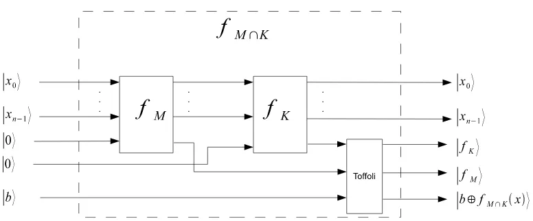
A straightforward algorithm for finding a member of the intersection between two sets of marked statesKandM, based on the oracles fKand fMinvolves the use of the intersection oracle, compris-ing the oracles in Equation 2, Equation 3 in sequence, and a Toffoli gate as depicted in Figure 6.
When the input to the oracle is|xi ⊗ |0i ⊗ |0i ⊗ |0i, then the output is|xi ⊗ |fK(x)i ⊗ |fM(x)i ⊗ |fK∩M(x)i. The intersection phase oracle is realized when|bi=|−i, then, the input|xi⊗|0i⊗|0i⊗ |−iwill cause the output to be|xi ⊗ |fK(x)i ⊗ |fM(x)i ⊗
(−1)fK∩M(x)|−i.
Retrieving a state in the intersection between the two sets is accomplished by using Grover’s quantum search algorithm with the phase versionIK∩M of the oracle fM∩K.
However, under certain conditions, one might not have the two oracles at hand, and, thus, the use of the intersection oracle might not be feasible. Another usage is when one constant oracle is available and the second oracle needs to be changed with each activation. We present an algorithm that applies a series of computations carried out by the two owners of the oracles in an alternating fashion.
Algorithm 1 : Quantum Set Intersection
Given: Phase oraclesIMandIK
Figure 6: The intersection oracleFK∩Mcreated using fM, fK, andTo f f oli.
2. Repeat
|Ψi=QK|Ψi
|Ψi=QM|Ψi T =Oq N
|K∩M|
times 3.Measure|Ψi
Algorithm 1 assumes that the size of the intersection set|K∩M|is known in order to determine the number of iterations. In the more general case where|K∩M|is unknown we apply the mod-ification for an unknown number of marked states (Boyer et al., 1996). Alteratively, we can use the quantum counting algorithm (Brassard et al., 1998) for the apriori estimation of the number of marked states. In both cases the time complexity of the set intersection algorithm is sub-exponential. Next, we present two theorems that prove that Algorithm 1 measures a member of the intersection set with maximal probability and this probability is asymptotically close to 1.
Theorem 1 Let IK and IM be phase oracles that mark two sets of n-qubit states K and M with
|K|,|M|<<N. Let us denote|K|=k,|M|=m,|K∩M|=r,
Q≡QMQK= (HI0HIMHI0HIK) (4)
and
|Ψ(t)i=QTH|0i.
Then, the maximal probability of measuring a state in the intersection K∩M is achieved at
T =arg max t x
∑
∈K∩M
|hx|Ψ(t)i|2=
π/2−arctanqNr−r
arccos 4Nkm2 −4Nr+Γ
(5)
where
Γ= r
1−8rN
3+8kmN2−16rkN2−16rmN2+32rkmN−16k2m2
Proof The Hilbert space spanned by all computational basis states of the n-qubit register can be divided into four different subspaces: the subspace spanned by the states inK∩M, the subspace spanned by the states inK\M, the subspace spanned by the states inM\K, and the subspace spanned by the states inK∪M. Accordingly, we select an orthonormal basis for representing the operator, in which the first four basis states are:
|l1i ≡ p 1
|K∩M|i∈
∑
K∩M|ii, (6)
|l2i ≡ p 1
|K\M|i∈
∑
K\M|ii, (7)
|l3i ≡ p 1
|M\K|i∈
∑
M\K|ii, (8) |l4i ≡ p 1|K∪M|i∈
∑
K∪M|ii (9)and the rest of the basis consists of orthonormal extensions of these states, then
H|0i= r
r N|l1i+
r
k−r N |l2i+
r
m−r
N |l3i+
r
N−m−k+r
N |l4i.
The operatorQKaffects only the four states(|l1i,|l2i,|l3i,|l4i)as follows:
QK|l1i= −HI0HIK|l1i=−H(I−2|0ih0|)H I−2
∑
i∈K|iihi|
!
|l1i=
1−2r N
|l1i+ −2 p
r(k−r)
N
!
|l2i
+ −2
p
r(m−r)
N
!
|l3i+ −2 p
r(N−m−k+r)
N
!
|l4i,
QK|l2i= −HI0HIK|l2i=−H(I−2|0ih0|)H I−2
∑
i∈K|iihi|
!
|l2i=
−2
p
r(k−r)
N
!
|l1i+
1−2(k−r) N
|l2i
+ −2
p
(k−r)(m−r)
N
!
|l3i+ −2 p
(k−r)(N−m−k+r)
N
!
QK|l3i= −HI0HIK|l3i=−H(I−2|0ih0|)H I−2
∑
i∈K|iihi|
!
|l3i=
2pr(m−r)
N
!
|l1i+ 2 p
(k−r)(m−r)
N
!
|l2i
+
2(m−r)
N −1
|l3i+ 2 p
(m−r)(N−m−k+r)
N
!
|l4i,
QK|l4i= −HI0HIK|l4i=−H(I−2|0ih0|)H I−2
∑
i∈K|iihi|
!
|l4i=
2pr(N−m−k+r)
N
!
|l1i+ 2 p
(k−r)(N−m−k+r)
N
!
|l2i
+ 2
p
(m−r)(N−m−k+r)
N
!
|l3i+
2(N−m−k−+r)
N −1
|l4i
yieldingQKin matrix form
QK=
1−2Nr −2
√
r√k−r N
2√r√m−r N
2√r√N−k−m+r N
−2√r√k−r
N 1−
2(k−r)
N
2√k−r√m−r N
2√k−r√N−k−m+r N
−2√r√m−r
N −
2√k−r√m−r N
2(m−r)
N −1
2√m−r√N−k−m+r N
−2√r√N−k−m+r
N −
2√k−r√N−k−m+r N
2√m−r√N−k−m+r N
2(N−k−m+r)
N −1
. (10)
Similarly, we obtain the matrix form ofQM
QM=
1−2Nr 2√r
√
k−r N
−2√r√m−r N
2√r√N−k−m+r N
−2√r√k−r N
2(k−r)
N −1 −
2√k−r√m−r N
2√k−r√N−k−m+r N
−2√r√m−r N
2√k−r√m−r N
1−2(m−r)
N
2√m−r√N−k−m+r N
−2√r√N−k−m+r N
2√k−r√N−k−m+r
N −
2√m−r√N−k−m+r N
2(N−k−m+r)
N −1
. (11)
Substituting Equation 10 and Equation 11 into Equation 4 yields
Q =
1−8r(NN−2m) −
4√r√k−r(N−2m)
N2 0 0
−4√r√k−r(N−2m)
N2
8m(k−r)
N2 −1 0 0 −8√r√m−r(N−m)
N2 −
4√k−s√m−r(N−2m)
N2 0 0
−4√r√N−k−m+r(N−2m)
N2
8m√k−r√N−k−m+r
N2 0 0
+
0 0 8√r
√
m−r(N−m)
N2
4√r√N−k−m+r(N−2m)
N2
0 0 4
√
k−r√m−r(N−2m)
N2 −
8m√k−r√N−k−m+r N2
0 0 8(N−mN)(2m−r)−1
4√m−r√N−k−m+r(N−2m)
N2
0 0 4
√
m−r√N−k−m+r(N−2m)
N2 1−
8m(N−k−m+r)
The compound operator Qis a rotation in the 4dimensional space spanned by Equations 6 -Equation 9. Finding the rotation angles requires the diagonalized matrix ofQ. LetV be the matrix whose columns are the eigenvectors ofQ, thenQD=V−1QV is a diagonal matrix whose diagonal components are the eigenvalues ofQas follows:
QD=
e−iw1 0 0 0
0 eiw1 0 0
0 0 e−iw2 0
0 0 0 eiw2
where
e−iw1 = 4km
N2 −
4r
N +Γ−∆
eiw1 = 4km
N2 −
4r
N +Γ+∆
e−iw2 = 4km
N2 −
4r
N −Γ−∆
eiw2 = 4km
N2 −
4r
N −Γ+∆
andΓand∆are given by
Γ =
r
1−8rN
3+8kmN2−16rkN2−16rmN2+32rkmN−16k2m2
N4 ,
∆ = 2
r
2N2r(r+k+m)−N3r(1+Γ) +N2kmΓ−N2km−8Nkmr+4k2m2 N4
which implies
w1 = arccos
4km
N2 −
4r
N +Γ
,
w2 = arccos
4km
N2 −
4r
N −Γ
.
The amplitude of|l1iis given by
a(t) =Asin(w1t+φ) (12)
whereAis the maximal amplitude, to be found, andφis the angle between the initial stateH|0i⊗n and|l1i:
φ=arctan
r
r N−r.
The maximal probabilityA2that a measurement of the system will produce a state inK∩Mwill be obtained at time
T =arg max t A
yielding
T =
π/2−arctanqN−rr arccos 4Nkm2 −4Nr+Γ
as asserted (Equation 5).
Theorem 1 suggests a way for approximating the time complexity of the algorithm whenm,k<< N. Employing the Taylor series, the second order approximation of the rotation angle is
w1=O
r
r N
and the number of iterations can be approximated by
T ≈O
π/2−qN−rr
pr
N
=O r
N r
!
. (13)
Theorem 2 The maximal probability, A2from Equation 12, of measuring a marked state in K∩M from Theorem 1 is approximately1when|K|,|M|<<N and N is large.
Proof The amplitudea(t)of|l1ibehaves as in Equation 12 and the maximal amplitudeAcan be obtained from
Asin(w1+φ) =
r
r N
1−8r(N−m) N2
+ r
k−r N
−4√r√k−r(N−2m)
N2
+ r
m−r
N
8√r√m−r(N−m)
N2
+ r
N−m−k+r N
4√r√N−m−k+r(N−2m)
N2
. (14)
A≈
pr
N
1−8r(NN−2m)
q
2−2Γ−8km N2 +8Nr+
q
r N−r
+ q
k−r N
−4√r√k−r(N−2m)
N2
q
2−2Γ−8km N2 +8Nr+
q
r N−r
+ q
m−r N
8√r√m−r(N−m)
N2
q
2−2Γ−8km N2 +8Nr+
q
r N−r
+ q
N−m−k+r N
4√r√N−m−k+r(N−2m)
N2
q
2−2Γ−8Nkm2 +
8r N +
q
r N−r
which, under the assumptionr,k,m<<N, is close to 1.
3. Quantum Associative Memory
In this section we introduce our associative memory model and the retrieval procedure with pattern completion and correction abilities. We present the concept of memory as a quantum operator that flips the phase of the memory patterns. The operator is based on an oracle that identifies, or ”marks”, memory patterns. This allows the initial state of our algorithm to be independent of the memory set. The input of our algorithms is ann-qubit register that contains the superposition of all basis states. This input is created by applying the Hadamard operation on ann-qubit register set to zeros,H|0i.
3.1 Pattern Completion
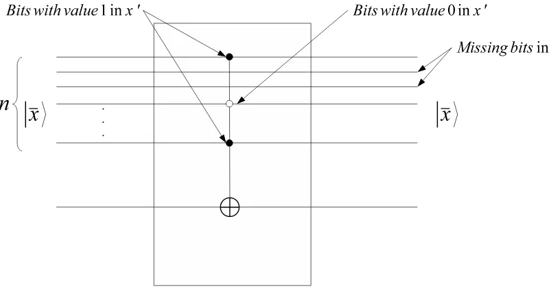
Let IM be a phase oracle on a set M, called the memory set, of m n-qubit patterns and let x′ be a version of a memory pattern x∈M with d missing bits. We are required to output the pattern x based on IM and x′. The partial pattern is given as a string of binary values 0 and 1 and some unknown bits marked ’?’. Denoting the set of possible completions of the partial pattern K and its size k, the completion problem can be reduced to the problem of retrieving a member x of the intersection between two sets K and M, x∈K∩M. For example, let M=
{0101010,0110100,1001001,1111000,1101100,1010101,0000111,0010010}be a 7-bit memory set of size 8 and let ”0110?0?” be a partial pattern with 2 missing bits, so the completion set is K={0110000,0110001,0110100,0110101}. Pattern completion is the computation of the inter-section betweenKandM, which is the memory pattern 0110100.
Figure 7: An implementation of a completion operator with an up ton+1 dimensional controlled-not operator.
to the corresponding qubit. The dark circle means that the control is activated when the bit value is 1 and the empty circle means that the control is activated when the bit value is 0. For each missing bit, no control is added for the corresponding qubit. A singlenqubit operator can be implemented byO(n)2 and 3-qubit operators (Barenco et al., 1995).
The algorithm for pattern completion through the quantum intersection algorithm is
Algorithm 2 : Quantum Pattern Completion
Given: A memory operatorIMand a patternx′∈ {0,1}n, which is a partial version
of some memory pattern with up todmissing bits
1. Create the completion operatorIK. 2. Apply Algorithm 1 with IMand IK
3.2 Pattern Correction
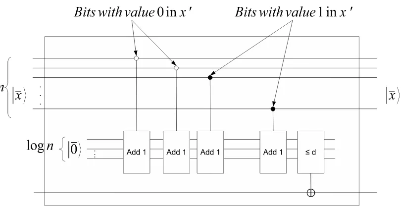
Figure 8: An implementation of a correction operator with a ⌈logn⌉additional bits, n controlled operators that add 1, and a threshold operator.
consists of all patterns that are in Hamming distance up to 2 fromx′. Pattern correction should then retrieve the memory pattern 0110100.
Pattern correction can be solved using the quantum intersection algorithm, which requires the creation of the correction operator fKor its phase versionIK. This can be implemented by checking whether the number of different bits between any given state and the faulty patternx′is less or equal tod. Such an implementation is shown in Figure 8. The operator applies a linear threshold on the hamming distance betweenx′and any inputx. The operator consists ofninput qubits,⌈logn⌉qubits for the hamming distance ofxfromx′, and an additional qubit for the output. The operator adds 1 for each bit inxthat is not equal to the corresponding bit inx′, then applies a controlled not operator if the hamming distance does not exceed the thresholdd. The operator can, thus, be implemented usingO(nlogn)2 and 3-qubit operators.
Algorithm 3 : Quantum Pattern Correction
Given: A memory operatorIMand a patternx′∈ {0,1}n, which is a faulty version of some memory pattern with up tod faulty bits
1. Create the correction operatorIK. 2. Apply Algorithm 1 with IMand IK
Algorithm 3 finds a memory pattern that is in Hamming distance up todfromx′. If the memory is within the correction capacity bounds, Algorithm 3 finds the correct patternxwith high probabil-ity, as will be proved in Section 4. However, if we are interested in ensuring that we find the closest memory pattern tox′, with no dependence on the capacity bound, then we can apply Algorithm 3 fori=0 bits and increase it up toi=dbits. In this case we ensure that we find a pattern x, such that
x:(x∈M)∧ ∀x′′∈M:dist(x′′,x)≥dist(x′,x)
wheredist(·,·)is the Hamming distance.
4. Analysis of the Quantum Associative Memory
In this section we analyze the time complexity and memory capacity of the proposed quantum as-sociative memory. We first show that the time complexity of retrieval operations is sub-exponential in the number of bits. Then we show that the number of memory patterns that can be stored while the model retains its correction and completion abilities is exponential in the number of bits.
4.1 Time Complexity Analysis
The time complexity of the retrieval procedure with either pattern completion or correction ability is determined by the complexity of the quantum intersection algorithm and the complexity of the completion and correction operators. The two operators can be implemented by a number of oper-ations which is linear innor in nlogn. According to Equation 13, the completion and correction operations are performed in
T ≈nlogn+O
s
N |K∩M|
!
=O
s
N |K∩M|
!
operations, which is sub-exponential in number of bits.
4.2 Capacity Analysis
We consider three different capacity measures. The first is the equilibrium capacityMeq, which is the maximal memory size that ensures that all memory patterns are equilibrium points of the model. An Equilibrium point is a pattern that, when presented to the model as an input, is also retrieved as an output with high probability. The second is the pattern completion capacityMcom, which is the maximal memory size that allows the completion of any partial pattern with up to d missing bits with high probability. The third is the pattern correction capacityMcor, which is the maximal memory size that allows the correction of any pattern with up todfaulty bits with high probability. Equilibrium is a special case of completion and correction with neither missing nor faulty bits. Therefore, the equilibrium capacity should be equal to the completion and correction capacities for d=0.
4.2.1 EQUILIBRIUMCAPACITY
The equilibrium capacity of the quantum associative memory is
because every memory state of ann-bit associative memoryMof any sizem≤Nis an equilibrium state, that is, ifQx=−(HI0HIx),T =
π
4 √
N, and|Ψ(T)i=QTxH|0i, then
∀x∈M: |hx|Ψ(T)i|2→1as n→∞.
This is a direct consequence of Grover’s algorithm (Grover, 1996) and the results obtained by Boyer et al. (1996) concerning the ability to find any member of the sizeNdatabase with probability close to 1.
4.2.2 COMPLETIONCAPACITY
Given a patternx′, which is a partial version of some memory patternxc withd missing bits, we seek the maximal memory size, for which the pattern can be completed with high probability from a random uniformly distributed memory set (McEliece et al., 1987; Baram, 1991; Baram and Sal’ee, 1992).
The completion capacity is bounded from above by two different bounds. The first is a result of Grover’s quantum search algorithm limitations and the second is a result of the probability of correct completion.
A Bound on Memory Size due to Grover’s Quantum Search Limitations. Grover’s operator flips the
marked states around the zero amplitude (negating their amplitudes) then flips all amplitudes around the average of all amplitudes (Biham et al., 1999). Amplification of the desired amplitudes occurs only when the average of all amplitudes is closer to the amplitudes of the non-marked states than to the marked states. This imposes the following upper bound on the memory size:
m<N/2.
This can be observed in the first iteration of the quantum search algorithm on a number of marked states. The initial amplitude of all basis states inH|0iis 1/√N. Flipping the phase ofm marked states byIMto−1/
√
Nyields an average amplitude of
(N−m)∗1/√N
−m∗
1/√N
=N√−2m
N .
Then, flipping the phases of all basis states around this average by HI0H yields two values of amplitudes. The amplitudes of marked and unmarked states become
2
N−2m
√ N
±√1
N =
2N−4m±1 √
N
(15)
where±correspond to marked and unmarked states respectively.
A necessary condition for the amplification of marked states is that the absolute value of their amplitudes after an iteration of the algorithm is higher than the absolute value of the amplitude of unmarked states. The condition is satisfied if and only if the two equations given in Equation 15 satisfy
2N−4m+1 √ N >
which holds true if and only ifm<N/2. Therefore, ifm≥N/2 the amplitudes of the marked states will not increase, which gives the following upper bound on the completion capacity:
Mcom<N/2. (16)
However, this is a very loose bound and the success probability of the completion will impose a tighter bound.
A Bound on Memory Size due to Pattern Completion.The bound on memory size that ensures a high
probability of correct completion depends on the definition of the pattern completion procedure. If one defines pattern completion as the process of outputting any of a number of possible memory patterns when given a partial input, then the capacity bound of our memory is the amplification bound given in Equation 16. However, this is not always the case. Pattern completion capacity is usually defined as the maximal size of a random uniformly distributed memory set that, given a partial versionx′of a memoryxc∈Mwithd missing bits, outputsxc. The following theorem gives an upper bound on the capacity for pattern completion with high probability:
Theorem 3 An n-bit associative memory with m random patterns can complete up to d missing bits on average when
m≤2n−d with probability higher than
v ev−1
m
∑
i=1 vi−1
ii (17)
as n grows to infinity, where
v= m
2n−d.
Proof LetMbe a random uniformly distributed memory set of sizem=v2n−d, where 0<v<1. Letx′be a partial pattern ofxc∈Mwithd missing bits.x′induces the set
K=
xx is a completion o f x′
where|K|=2d. LetZibe random indicator variables representing the existence of theith member ofMinK. Denotingp=Pr(Zi=1) =2
d
2n =2n1−d, we have
m=v/p. (18)
Let us denote|Ψ(T)i=QTH|0iandS=∑mi=1Zi. If there is only one possible memory completion, then it isxc, and if there are two, thenxc is one of the two, and so on. Therefore, the probability of successfully outputtingxc from the partial patternx′ is the sum of the conditional probabilities that there areimemory completions divided byi:
|hxc|Ψ(T)i|2 = m
∑
i=1
Pr(S=i|S≥1)
i
=
m
∑
i=1
Pr(S=i)
iPr(S≥1) =
m
∑
i=1 m
i
pi(1−p)m−i
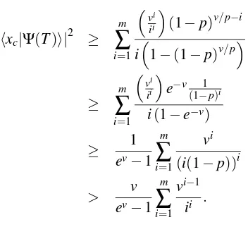
Now, this probability can be lower-bounded by
|hxc|Ψ(T)i|2≥ m
∑
i=1 m
i
i
pi(1−p)m−i
i(1−(1−p)m) . (20)
Substituting Equation 18 in Equation 20 we have
|hxc|Ψ(T)i|2 ≥ m
∑
i=1
vi
ii
(1−p)v/p−i
i
1−(1−p)v/p
≥ m
∑
i=1
vi ii
e−v(1−1p)i
i(1−e−v) ≥ 1
ev−1 m
∑
i=1 vi
(i(1−p))i
> v
ev−1 m
∑
i=1 vi−1
ii . (21)
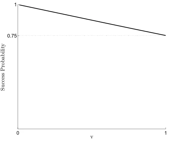
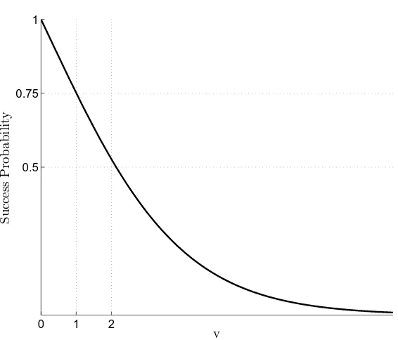
Figure 9 shows that the lower bound with approximation by only three terms of the sum in Equation 17 as a function ofv is higher than 75% for all possible sizes of a non-empty memory within the capacity limits.
Theorem 3 implies thatMcom(d) =2n−d, which agrees with the result concerning the equilib-rium capacity, sinceMcom(0) =2n−0=2n=N=Meq.
4.2.3 CORRECTIONCAPACITY
A bound on the correction capacity of Algorithm 3 is given be the following theorem:
Theorem 4 An n-bit associative memory with m random patterns can correct up to d faulty bits on average when
m≤2n−d/
n d
with probability higher than
v ev−1
m
∑
i=1 vi−1
ii
as n grows to infinity, where
v= m
2n−d.
Proof LetMbe a random uniformly distributed memory set of size
m=v2n−d/
n d
0 1 0.75
1
v
S
u
cc
es
s
P
ro
b
a
b
il
it
y
Figure 9: Success probability of pattern completion vs. memory size divided by the maximal com-pletion capacityvfor an associative memory withn=30 qubits.
where 0<v<1. Letx′be a patternxc∈Mwithdfaulty bits.x′induces a set
D=
xdist(x,x′)≤d
where|D|= dn
2d. LetZibe random indicator variables representing the existence of theith mem-ber ofMinD. Denotingp=Pr(Zi=1) = nd
2d−n, we have m=v/p.
Let us denote|Ψ(T)i=QTH|0iandS=∑mi=1Zi. The probability of successfully retrievingxcfrom the patternx′is then
|hxc|Ψ(T)i|2= m
∑
i=1
Pr(S=i|S≥1)
i
which, according to Equations 19 - 21, also satisfies
|hxc|Ψ(T)i|2≥ v ev−1
m
∑
i=1 vi−1
ii .
Theorem 4 yieldsMcor(d) = nd
2n−d, which also agrees with the result concerning the equilib-rium capacity, sinceMcor(0) = n0
2n−0=2n=N=M eq.
0 1 2 0.75
0.5 1
v
S
u
cc
es
s
P
ro
b
a
b
il
it
y
Figure 10: Pattern completion or correction probability vs. the memory size divided by the maximal completion capacityv. For 0<v<1, the probability is above 75% and forv<2 is above 50%.
4.2.4 INCREASINGMEMORYSIZEBEYOND THECAPACITYBOUNDS
The various capacities presented above are exponential innunder the assumptiond<<n. However, an increase ofmbeyond the capacity bound results in a decay of the correct completion probability as depicted in Figure 10. It can be seen that it is more likely to find the correct completion than not to find it as long asv<2.
In addition, the model can also output a superposition of a number of possible outputs, by skipping the measurement operation in Algorithm 1. This is not true for most classical memory models where spurious memories arise and the output is usually not a memorized pattern, but, rather, some spurious combination of multiple memory patterns (Hopfield, 1982; Bruck, 1990; Goles and Mart´ınez, 1990).
5. Comparison to Previous Works
0 N/4 N 0
0.1 0.2 0.3 0.4 0.5 0.6 0.7 0.8 0.9 1
|M|
S
u
cc
es
s
P
ro
b
a
b
il
it
y
Figure 11: Memory size vs. success probability of Algorithm 4. Optimal results are achieved only when the memory size is close to N4.
Algorithm 4 The algorithm proposed by Ventura and Martinez (2000)
Given: Phase oraclesIMandIK
1. DenoteQM=−HI0HIMandQK=−HI0HIK 2. Let|Ψi= 1
m∑ m i=1|ii. 3. ApplyQMQKon|Ψi 4. ApplyQK on|ΨiforT=
j
π/4pN/|K∩M| k
-2times. 5. Measure|Ψi.
Algorithm 5 The algorithm proposed by Arima et al. (2009)
Given: Phase oraclesIMandIK
1. DenoteQM=−HI0HIMandQK=−HI0HIK 2. Let|Ψi= 1
m∑ m i=1|ii.
3. ApplyQMQKon|ΨiforTtimes. (Twas not found by Arima et al., 2009) 4. Measure|Ψi.
0 N/4 N2 N 0
0.1 0.2 0.3 0.4 0.5 0.6 0.7 0.8 0.9 1
|M|
S
u
cc
es
s
P
ro
b
a
b
il
it
y
Figure 12: Memory size vs. success probability in Algorithm 5. Satisfactory results are achieved only when the memory size exceedsN4.
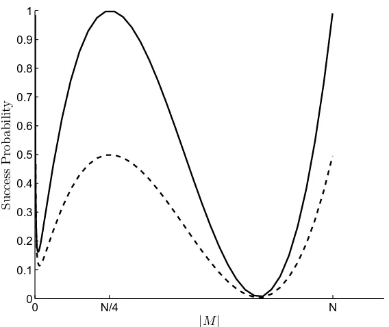
Algorithm 5 gives satisfying results only when the memory size exceedsN4, which is exponential in the number of qubits, leaving the possibility of effective pattern completion only for 2 qubits or less. It is therefore not helpful for associative memory with pattern completion and correction abilities. The success probability of Algorithm 5 vs. the memory size is depicted in Figure 12. Miyajima et al. (2010) added a control parameter to tune the algorithm, changing the memory size for which the maximal amplitude is achieved. The algorithm is presented only for one marked state with no completion and correction abilities. The time complexity and stopping criteria were not stated by Arima et al. (2008) and were later found to be O √N (Arima et al., 2009; Miyajima et al., 2010).
Our algorithm, on the other hand achieves high success probability up to memory size N4, as depicted in Figure 13.
Furthermore, both Algorithm 4 and Algorithm 5 need to initialize the system at a superposition of the memory states:
|Ψi=√1
m m
∑
i=1 |ii
0 N/4 N/2 N 0
0.1 0.2 0.3 0.4 0.5 0.6 0.7 0.8 0.9 1
|M|
S
u
cc
es
s
P
ro
b
a
b
il
it
y
Figure 13: Memory size vs. success probability in Algorithms 2 and 3.
a multiple number of times. Our algorithm’s initialization, on the other hand, does not depend on the memory patterns.
6. Numerical Examples and Simulations
Let us first consider an associative memory of 10 qubits. We have randomly chosen a set of 50 patternsMout of the possible 1024 to be stored in memory. We also chose two partial patterns, each with 4 missing qubits, yielding two completion setsK1andK2of 16 possible completions each. We choseK1andK2such that they have one and two completions in memory respectively. Figure 14(a) shows the memory set, where each vertical line represents a memory pattern, and Figure 14(b) shows the completion setK1in the same manner. The amplitudes of the final state of the completion algorithm are shown in Figure 14(c), where the only possible memory completion has amplitude close to 1. Figure 15 shows the high amplitudes of the two possible memory completions when the completion set isK2.
As can be seen, applying our algorithm to both completion sets amplified the states that are possible completions in memory. The amplitudes of the desired states reached up to 96.76% in the first case and 68.44% in the second case for each one of the two high amplitudes. Therefore, the probability of measuring the correct completion in the first case is 93.62% and the probability of measuring one of the two correct completions in the second case is 93.67%.
0 200 400 600 800 1000
0 200 400 600 800 1000
0 200 400 600 800 1000
0 1
K1
M∩K1 M
(a)
(c)
(b)
Figure 14: (a) A set of memory patternsM(b) a set of possible completionsK1to a partial pattern, and (c) the memory completion result in amplitudes.
0 200 400 600 800 1000
0 200 400 600 800 1000
0 200 400 600 800 1000
0 1
M
K2
M∩K2
(a)
(b)
(c)
−1 0 1
NOT(K∪M) K∩M
K\M M\K
Figure 16: Simulation of a series of iterations of the completion algorithm. The graph shows the different behavior of the different subgroups of basis states.Kis the completion set and Mis the memory set. The memory completions and the non completions or memories are amplified alternatingly, while the amplitudes ofK\MandM\Ksubgroups stay close to zero.
groupK∩M and inNOT(K∪M)alternatingly, while the amplitudes of states inK\M andM\K stay close to zero.
We have also tested our algorithms with a larger number of qubits in order to verify that the success rate of retrieval grows asymptotically to 1 as the number of qubits grows. For instance, we tested a 30 qubit system with 225 memory patterns and a completion query that has 8 missing bits. We tested different completions of 8 missing bits so that the intersection set size varied from 1 to 10 patterns. Our algorithm found a member of the memory completion set with probability 96.8%. Increasing the memory size to 226 and 227, and thereby bringing the capacity close to its limit resulted in completion probabilities of 93.5% and 86.7% respectively. Figure 17 depicts the success rates of pattern completion in a 30 qubit system. An explanation of the different graphs can be found in Table 1. The solid line in Figure 17 depicts the success probability vs. the logarithm of the size of memory with completion queries set to 8 missing bits and the number of possible memory completions set to 1. The dashed line depicts the success probability vs. the logarithm of the completion query size when the memory size is set to 225 patterns and the number of possible memory completions set to 1. The dotted line depicts the success probability vs. the logarithm of the number of possible memory completions when both the memory size and the completion query size are set to 225. The dash-dotted line depicts the success probability vs. the number of qubits in the system (growing from 5 to 30 qubits) when the memory size, the completion query size, and the number of possible memory completions are small constants.
Further-Graph |N| |M| |K| |K∩M|| Solid constant varying constant constant —— 230 23−227 23 1 Dashed constant constant varying constant
– – – 230 225 23−225 1 Dotted constant constant constant varying
··· 230 225 225 1−225 Dash-dotted varying constant constant constant
–·–·– 25−230 23 23 1
Table 1: Properties of the four simulations depicted in Figure 17. Thexaxis in Figure 17 represents the varying set size, while the other set sizes are constant in each simulation.
0 5 10 15 20 25 30
0.75 1
S
u
cc
es
s
P
ro
b
a
b
il
it
y
more, the success probability increases when the number of possible memory completions (the size of the intersection set) grows towards the sizes of the completion query and the memory, which indicates that choosing a member of the intersection becomes easy (by randomly choosing a possi-ble completion). Finally, the figure also shows that, as the number of qubits in the system grows, the success probability becomes asymptotically 1, which indicates that, practically, our algorithm produces the intersection whenn>>1.
7. Conclusion
We have presented a quantum computational algorithm that computes the intersection between two subsets ofn-bit strings. The algorithm is based on a modification of Grover’s quantum search. Us-ing the intersection algorithm, we have presented a set of algorithms that implement a model of associative memory via quantum computation. We introduced the notion of memory as a quantum operator, thus avoiding the dependence of the initial state of the system on the memory set. We have shown that our algorithms have both speed and capacity advantages with respect to classical asso-ciative memory models, consuming sub-exponential time, and are able to store a number of memory patterns which is exponential in the number of bits. Pattern retrieval algorithms with completion and correction abilities were presented. Bounds relating memory capacity to the maximal allowed signal to noise ratio were found.
References
K. Arima, H. Miyajima, N. Shigei, and M. Maeda. Some properties of quantum data search algo-rithms. InProceedings of the The 23rd International Technical Conference on Circuits/Systems, Computers and Communication (ITC-CSCC2008), pages 1169–1172, 2008.
K. Arima, N. Shigei, and H. Miyajima. A proposal of a quantum search algorithm. International Conference on Convergence Information Technology, 0:1559–1564, 2009.
Y. Baram. On the capacity of ternary hebbian networks. Information Theory, IEEE Transactions on, 37(3):528–534, May 1991.
Y. Baram and D. Sal’ee. Lower bounds on the capacities of binary and ternary networks storing sparse random vectors. Information Theory, IEEE Transactions on, 38(6):1633 –1647, nov 1992. A. Barenco, C. H. Bennett, R. Cleve, D. P. DiVincenzo, N. H. Margolus, P. W. Shor, T. Sleator, J. A. Smolin, and H. Weinfurter. Elementary gates for quantum computation. Physical Review A, 52 (5):3457–3467, 1995.
E. Biham, O. Biham, D. Biron, M. Grassl, and D. A. Lidar. Grover’s quantum search algorithm for an arbitrary initial amplitude distribution. Physical Review A, 60(4):2742–2745, 1999.
M. Boyer, G. Brassard, P. H ¨oyer, and A. Tapp. Tight bounds on quantum searching. Technical Report PP-1996-11, 30, 1996.
J. Bruck. On the convergence properties of the hopfield model. Proceedings of the IEEE, 78(10): 1579–1585, oct 1990.
D. Deutsch. Quantum theory, the church-turing principle and the universal quantum computer. Proceedings of the Royal Society A Mathematical Physical and Engineering Sciences, 400:97– 117, 1985.
D. Deutsch and R. Jozsa. Rapid solution of problems by quantum computation.Proceedings Math-ematical and Physical Sciences, 439(1907):553–558, 1992.
A. Ezhov, A. Nifanova, and D. Ventura. Quantum associative memory with distributed queries. Inf. Sci. Inf. Comput. Sci., 128(3-4):271–293, 2000.
E. Goles and S. Mart´ınez. Neural and Automata Networks: Dynamical Behavior and Applications. Kluwer Academic Publishers, 1990.
L. K. Grover. A fast quantum mechanical algorithm for database search. InSTOC ’96: Proceedings of the Twenty-eighth Annual ACM Symposium on Theory of Computing, pages 212–219, 1996.
J. Hopfield. Neural networks and physical systems with emergent collective computational abilities. Proceedings of the National Academy of Sciences of the United States of America, 79:2554–2558, 1982.
J. C. Howell, J. A. Yeazell, and D. Ventura. Optically simulating a quantum associative memory. Physical Review A, 62(4):042303, 2000.
P. Kanerva. Sparse distributed memory and related models. InAssociative Neural Memories, pages 50–76. Oxford University Press, 1993.
R. McEliece, E. Posner, E. Rodemich, and S. Venkatesh. The capacity of the hopfield associative memory. Information Theory, IEEE Transactions on, 33(4):461–482, jul 1987.
H. Miyajima, N. Shigei, and K. Arima. Some quantum search algorithms for arbitrary initial ampli-tude distribution. InSixth International Conference on Natural Computation (ICNC), volume 8, pages 603–608, 2010.
M.A. Nielsen and I.L. Chuang.Quantum Computation and Quantum Information. Cambridge Univ. Press, 2000.
P. W. Shor. Algorithms for quantum computation: Discrete logarithms and factoring. InProceedings of the IEEE Symposium on Foundations of Computer Science, pages 124–134, 1994.
D.R. Simon. On the power of quantum computation. InFoundations of Computer Science, 1994 Proceedings., 35th Annual Symposium on, pages 116 –123, nov 1994.