Feature Selection via Dependence Maximization

Feature Selection via Dependence Maximization

Le Song LSONG@CC.GATECH.EDU

Computational Science and Engineering Georgia Institute of Technology

266 Ferst Drive

Atlanta, GA 30332, USA

Alex Smola ALEX@SMOLA.ORG

Yahoo! Research 4301 Great America Pky Santa Clara, CA 95053, USA

Arthur Gretton∗ ARTHUR.GRETTON@GMAIL.COM

Gatsby Computational Neuroscience Unit 17 Queen Square

London WC1N 3AR, UK

Justin Bedo† JUSTIN.BEDO@NICTA.COM.AU

Statistical Machine Learning Program National ICT Australia

Canberra, ACT 0200, Australia

Karsten Borgwardt KARSTEN.BORGWARDT@TUEBINGEN.MPG.DE

Machine Learning and Computational Biology Research Group Max Planck Institutes

Spemannstr. 38

72076 T¨ubingen, Germany

Editor: Aapo Hyv¨arinen

Abstract

We introduce a framework for feature selection based on dependence maximization between the selected features and the labels of an estimation problem, using the Hilbert-Schmidt Independence Criterion. The key idea is that good features should be highly dependent on the labels. Our ap-proach leads to a greedy procedure for feature selection. We show that a number of existing feature selectors are special cases of this framework. Experiments on both artificial and real-world data show that our feature selector works well in practice.

Keywords: kernel methods, feature selection, independence measure, Hilbert-Schmidt indepen-dence criterion, Hilbert space embedding of distribution

1. Introduction

In data analysis we are typically given a set of observations X =_{x1, . . . ,xm} ⊆

X

which can be

used for a number of tasks, such as novelty detection, low-dimensional representation, or a range of

supervised learning problems. In the latter case we also have a set of labels Y=_{y1, . . . ,ym} ⊆

Y

at

our disposition. Tasks include ranking, classification, regression, or sequence annotation. While not always true in practice, we assume in the following that the data X and Y are drawn independently and identically distributed (i.i.d.) from some underlying distribution Pr(x,y).

We often want to reduce the dimension of the data (the number of features) before the actual learning (Guyon and Elisseeff, 2003); a larger number of features can be associated with higher data collection cost, more difficulty in model interpretation, higher computational cost for the classifier, and sometimes decreased generalization ability. In other words, there often exist motives in addition to finding a well performing estimator. It is therefore important to select an informative feature subset.

The problem of supervised feature selection can be cast as a combinatorial optimization prob-lem. We have a full set of features, denoted by

S

(each element in

S

corresponds to one dimension of the data). It is our aim to select a subset

T

⊆

S

such that this subset retains the relevant infor-mation contained in X . Suppose the relevance of a feature subset (to the outcome) is quantified by

Q

(

T

), and is computed by restricting the data to the dimensions in

T

. Feature selection can then be formulated as

T0

=arg max

T⊆S

Q

(

T

)subject to|

T

| ≤t, (1)

where_{| · |}computes the cardinality of a set and t is an upper bound on the number of selected fea-tures. Two important aspects of problem (1) are the choice of the criterion

Q

(

T

)and the selection algorithm.

1.1 Criteria for Feature Selection

A number of quality functionals

Q

(

T

)are potential candidates for feature selection. For instance, we could use a mutual information-related quantity or a Hilbert Space-based estimator. In any case, the choice of

Q

(

T

)should respect the underlying task. In the case of supervised learning, the goal is to estimate a functional dependence f from training data such that f predicts well on test data. Therefore, a good feature selection criterion should satisfy two conditions:

I:

Q

(

T

)is capable of detecting desired (linear or nonlinear) functional dependence between the data and the labels.

II:

Q

(

T

) is concentrated with respect to the underlying measure. This guarantees with high probability that detected functional dependence is preserved in test data.

HSIC has good uniform convergence guarantees, and an unbiased empirical estimate. As we show in Section 2, HSIC satisfies conditions I and II required for

Q

(

T

).

1.2 Feature Selection Algorithms

Finding a global optimum for (1) is typically NP-hard (Weston et al., 2003), unless the criterion is easily decomposable or has properties which make approximate optimization easier, for example, submodularity (Nemhauser et al., 1978; Guestrin et al., 2005). Many algorithms transform (1) into a continuous problem by introducing weights on the dimensions (Weston et al., 2000; Bradley and Mangasarian, 1998; Weston et al., 2003; Neal, 1998). These methods perform well for linearly sep-arable problems. For nonlinear problems, however, the optimisation usually becomes non-convex and a local optimum does not necessarily provide good features. Greedy approaches, such as for-ward selection and backfor-ward elimination, are often used to tackle problem (1) directly. Forfor-ward selection tries to increase

Q

(

T

)as much as possible for each inclusion of features, and backward elimination tries to achieve this for each deletion of features (Guyon et al., 2002). Although for-ward selection is computationally more efficient, backfor-ward elimination provides better features in general since the features are assessed within the context of all others present. See Section 7 for experimental details.

In principle, the Hilbert-Schmidt independence criterion can be employed for feature selection using either a weighting scheme, forward selection or backward selection, or even a mix of several strategies. While the main focus of this paper is on the backward elimination strategy, we also discuss the other selection strategies. As we shall see, several specific choices of kernel function will lead to well known feature selection and feature rating methods. Note that backward elimination using HSIC (BAHSIC) is a filter method for feature selection. It selects features independent of a particular classifier. Such decoupling not only facilitates subsequent feature interpretation but also speeds up the computation over wrapper and embedded methods.

We will see that BAHSIC is directly applicable to binary, multiclass, and regression problems. Most other feature selection methods are only formulated either for binary classification or regres-sion. Multiclass extensions of these methods are usually achieved using a one-versus-the-rest strat-egy. Still fewer methods handle classification and regression cases at the same time. BAHSIC, on the other hand, accommodates all these cases and unsupervised feature selection in a principled way: by choosing different kernels, BAHSIC not only subsumes many existing methods as special cases, but also allows us to define new feature selectors. This versatility is due to the generality of HSIC. The current work is built on earlier presentations by Song et al. (2007b,a). Compared with this earlier work, the present study contains more detailed proofs of the main theorems, proofs of secondary theorems omitted due to space constraints, and a number of additional experiments.

particular variants of HSIC as their feature relevance criterion. Finally, Sections 7–9 contain our ex-periments, where we apply HSIC to a number of domains, including real and artificial benchmarks, brain computer interface data, and microarray data.

2. Measures of Dependence

We begin with the simple example of linear dependence detection, and then generalize to the

de-tection of more general kinds of dependence. Consider spaces

X

⊂Rd _and

_Y

_⊂Rl_{, on which we}

jointly sample observations(x,y)from a distribution Pr(x,y). Denote by

C

xythe covariance matrix

C

xy=Exy

h

xy⊤i₋E_x[x]E_yh_y⊤i_{, (2)}

which contains all second order dependence between the random variables. A statistic that effi-ciently summarizes the degree of linear correlation between x and y is the Frobenius norm of

C

xy.

Given the singular valuesσiof

C

xythe norm is defined as

k

C

xyk2Frob:=

∑

i

σ2

i =tr

C

xy

C

xy⊤.

This quantity is zero if and only if there exists no linear dependence between x and y. This statistic is limited in several respects, however, of which we mention two: first, dependence can exist in forms other than that detectable via covariance (and even when a second order relation exists, the full extent of the dependence between x and y may only be apparent when nonlinear effects are included). Second, the restriction to subsets ofRd _{excludes many interesting kinds of variables,}

such as strings and class labels. In the next section, we generalize the notion of covariance to nonlinear relationships, and to a wider range of data types.

2.1 Hilbert-Schmidt Independence Criterion (HSIC)

In general

X

and

Y

will be two domains from which we draw samples(x,y): these may be real val-ued, vector valval-ued, class labels, strings (Lodhi et al., 2002), graphs (G¨artner et al., 2003), dynamical systems (Vishwanathan et al., 2007), parse trees (Collins and Duffy, 2001), images (Sch¨olkopf, 1997), and any other domain on which kernels can be defined. See Sch¨olkopf et al. (2004) and Sch¨olkopf and Smola (2002) for further references.

We define a (possibly nonlinear) mapping φ:

X

_→

F

from each x_∈

X

to a feature space

F

(and an analogous mapψ:

Y

→

G

wherever needed). In this case we may write the inner product

between the features via the positive definite kernel functions

k(x,x′):=

φ(x),φ(x′)

and l(y,y′):=

ψ(y),ψ(y′) .

The kernels k and l are associated uniquely with respective reproducing kernel Hilbert spaces

F

and

G

(although the feature mapsφandψmay not be unique). For instance, if

X

=Rd_{, then this}

could be as simple as a set of polynomials of order up to b in the components of x, with kernel k(x,x′) = (_hx,x′_i+a)b_{. Other kernels, like the Gaussian RBF kernel correspond to infinitely large}

We may now define a cross-covariance operator1 between these feature maps, in accordance with Baker (1973) and Fukumizu et al. (2004): this is a linear operator

C

xy:

G

7−→

F

such that

C

xy:=Exy[(φ(x)−µx)⊗(ψ(y)−µy)] where µx=Ex[φ(x)]and µy=Ey[ψ(y)].

Here_⊗denotes the tensor product. We need to extend the notion of a Frobenius norm to operators. This leads us to the Hilbert-Schmidt norm, which is given by the trace of

C

xy

C

xy⊤. For operators with

discrete spectrum this amounts to computing theℓ2norm of the singular values. We use the square of

the Hilbert-Schmidt norm of the cross-covariance operator (HSIC),_k

C

xyk2HSas our feature selection

criterion

Q

(

T

). Gretton et al. (2005a) show that HSIC can be expressed in terms of kernels as

HSIC(

F

,

G

,Pr

xy):=k

C

xyk 2

HS (3)

=E_xx′_yy′[k(x,x′)l(y,y′)] +E_xx′[k(x,x′)]E_yy′[l(y,y′)]−2E_xy[E_x′[k(x,x′)]E_y′[l(y,y′)]].

This allows us to compute a measure of dependence between x and y simply by taking expectations over a set of kernel functions k and l with respect to the joint and marginal distributions in x and y without the need to perform density estimation (as may be needed for entropy based methods).

2.2 Estimating the Hilbert-Schmidt Independence Criterion

We denote by Z= (X,Y) the set of observations_{(x1,y1), . . . ,(xm,ym)}which are drawn iid from

the joint distribution Prxy. We denote by EZ the expectation with respect Z as drawn from Prxy.

Moreover, K,L_∈Rm×m_{are kernel matrices containing entries Ki j =k(xi,xj) and Li j =l(yi,yj).}

Finally, H=I₋m−111_∈Rm×m_{is a centering matrix which projects onto the space orthogonal to}

the vector 1.

Gretton et al. (2005a) derive estimators of HSIC(

F

,G,Prxy)which have O(m−1)bias and they

show that this estimator is well concentrated by means of appropriate tail bounds. For completeness we briefly restate this estimator and its properties below.

Theorem 1 (Biased estimator of HSIC Gretton et al., 2005a) The estimator

HSIC0(

F

,G,Z):= (m−1)−2tr KHLH (4)

has bias O(m−1), that is, HSIC(

F

,G,Prxy)−EZ[HSIC0(

F

,G,Z)] =

O

(m−1).

This bias arises from the self-interaction terms which are present in HSIC0, that is, we still have

O(m) terms of the form Ki jLil and KjiLli present in the sum, which leads to the O(m−1) bias.

To address this, we now devise an unbiased estimator which removes those additional terms while ensuring proper normalization. Our proposed estimator has the form

HSIC1(

F

,

G

,Z):=

1 m(m₋3)

tr(K ˜˜L) + 1⊤K11˜ ⊤L1˜ (m₋1)(m₋2)−

2 m₋21

⊤_{K ˜}˜_L1

, (5)

where ˜K and ˜L are related to K and L by ˜Ki j= (1−δi j)Ki jand ˜Li j= (1−δi j)Li j(i.e., the diagonal

entries of ˜K and ˜L are set to zero).

1. We abuse the notation here by using the same subscript in the operatorCxyas in the covariance matrix of (2), even

Theorem 2 (Unbiased estimator of HSIC) The estimator HSIC1 is unbiased, that is, we have

E_Z[HSIC1(

_F

_,

_G

_{,Z)] =HSIC(}

_F

_,G,Prxy).

Proof We prove the claim by constructing unbiased estimators for each term in (3). Note that we

have three types of expectations, namelyE_xyE_x′_y′, a partially decoupled expectationE_xyE_x′E_y′, and E_xE_yE_x′E_y′, which takes all four expectations independently.

If we want to replace the expectations by empirical averages, we need to take care to avoid using the same discrete indices more than once for independent random variables. In other words, when taking expectations over n independent random variables, we need n-tuples of indices where each index occurs exactly once. We define the sets im_n to be the collections of indices satisfying this property. By simple combinatorics one can see that their cardinalities are given by the Pochhammer symbols(m)n=_(mm!_−n)!. Jointly drawn random variables, on the other hand, share the same index.

For the joint expectation over pairs we have

E_xyE_x′_y′k(x,x′)l(y,y′)= (m)−₂1E_Z

h

∑

(i,j)∈im

2

Ki jLi j i

= (m)−1 2 EZ

tr ˜K ˜L

. (6)

Recall that we set ˜Kii =L˜ii =0. In the case of the expectation over three independent terms E_xyE_x′E_y′[k(x,x′)l(y,y′)]we obtain

(m)−₃1E_Z h

∑

(i,j,q)∈im3

Ki jLiq i

= (m)−₃1E_Z h

1⊤K ˜˜L1₋tr ˜K ˜L i

. (7)

For four independent random variablesE_xE_yE_x′E_y′[k(x,x′)l(y,y′)],

(m)−1 4 EZ

h

∑

(i,j,q,r)∈im

4

Ki jLqr i

= (m)−1 4 EZ

h

1⊤K11˜ ⊤L1˜ ₋41⊤K ˜˜L1+2 tr ˜K ˜Li. (8)

To obtain an expression for HSIC we only need to take linear combinations using (3). Collecting terms related to tr ˜K ˜L, 1⊤K ˜˜L1, and 1⊤K11˜ ⊤L1 yields˜

HSIC(

F

,G,Pr

xy) =

1 m(m₋3)EZ

tr ˜K ˜L+ 1⊤K11˜ ⊤L1˜ (m₋1)(m₋2)−

2 m₋21

⊤_{K ˜}˜_L1

. (9)

This is the expected value of HSIC1[

F

,

G

,Z].

Note that neither HSIC0 nor HSIC1 require any explicit regularization parameters, unlike earlier

work on kernel dependence estimation. Rather, the regularization is implicit in the choice of the kernels. While in general the biased HSIC is acceptable for estimating dependence, bias becomes a significant problem for diagonally dominant kernels. These occur mainly in the context of sequence analysis such as texts and biological data. Experiments on such data (Quadrianto et al., 2009) show that bias removal is essential to obtain good results.

For suitable kernels HSIC(

F

,

G

,Prxy) =0 if and only if x and y are independent. Hence the

empirical estimate HSIC1can be used to design nonparametric tests of independence. A key feature

is that HSIC1 itself is unbiased and its computation is simple. Compare this to quantities based

on the mutual information, which requires sophisticated bias correction strategies (e.g., Nemenman et al., 2002).

2.3 HSIC Detects Arbitrary Dependence (Property I)

Whenever

F

,G are RKHSs with characteristic kernels k,l (in the sense of Fukumizu et al., 2008; Sriperumbudur et al., 2008, 2010), then HSIC(

F

,G,Prxy) =0 if and only if x and y are

indepen-dent.2 In terms of feature selection, a characteristic kernel such as the Gaussian RBF kernel or the

Laplace kernel permits HSIC to detect any dependence between

X

and

Y

. HSIC is zero only if

features and labels are independent. Clearly we want to reach the opposite result, namely strong dependence between features and labels. Hence we try to select features that maximize HSIC. Likewise, whenever we want to select a subset of features from X we will try to retain maximal dependence between X and its reduced version.

Note that non-characteristic and non-universal kernels can also be used for HSIC, although they may not guarantee that all dependence is detected. Different kernels incorporate distinctive prior knowledge into the dependence estimation, and they focus HSIC on dependence of a certain type. For instance, a linear kernel requires HSIC to seek only second order dependence, whereas a polynomial kernel of degree b restricts HSIC to test for dependences of degree (up to) b. Clearly HSIC is capable of finding and exploiting dependence of a much more general nature by kernels on graphs, strings, or other discrete domains. We return to this issue in Section 5, where we describe the different kernels that are suited to different underlying classification tasks.

2.4 HSIC is Concentrated (Property II)

HSIC1, the estimator in (5), can be alternatively formulated using U-statistics (Hoeffding, 1948).

This reformulation allows us to derive a uniform convergence bound for HSIC1. Thus for a given

set of features, the feature quality evaluated using HSIC1closely reflects its population counterpart

HSIC.

Theorem 3 (U-statistic of HSIC) HSIC1can be rewritten in terms of a U-statistic

HSIC1(

F

,G,Z) = (m)−₄1

∑

(i,j,q,r)∈im4

h(i,j,q,r), (10)

where the kernel h of the U-statistic is defined by

h(i,j,q,r) = 1

24

(i,j,q,r)

∑

(s,t,u,v)

Kst[Lst+Luv−2Lsu] (11)

=1

6

(i,j,q,r)

∑

(s_≺t),(u_≺v)

Kst[Lst+Luv]−

1 12

(i,j,q,r)

∑

(s,t,u)

KstLsu. (12)

Here the first sum represents all 4!=24 quadruples(s,t,u,v) which can be selected without re-placement from(i,j,q,r). Likewise the sum over(s,t,u)is the sum over all triples chosen without replacement. Finally, the sum over(s_≺t),(u_≺v) has the additional condition that the order im-posed by(i,j,q,r)is preserved. That is(i,q)and(j,r) are valid pairs, whereas(q,i)or(r,q)are not.

2. This result is more general than the earlier result of Gretton et al. (2005a, Theorem 4), which states that whenF,G are RKHSs with universal kernels k,l in the sense of Steinwart (2001), on respective compact domainsX andY , then HSIC(F,G,Prxy) =0 if and only if x and y are independent. Universal kernels are characteristic on compact

Proof Combining the three unbiased estimators in (6-8) we obtain a single U-statistic

HSIC1(

F

,G,Z) = (m)−₄1

∑

(i,j,q,r)∈im

4

(Ki jLi j+Ki jLqr−2Ki jLiq). (13)

In this form, however, the kernel h(i,j,q,r) =Ki jLi j+Ki jLqr−2Ki jLiq is not symmetric in its

arguments. For instance h(i,j,q,r)=₆ h(q,j,r,i). The same holds for other permutations of the indices. Thus, we replace the kernel with a symmetrized version, which yields

h(i,j,q,r):= 1

4!

(i,j,q,r)

∑

(s,t,u,v)

(KstLst+KstLuv−2KstLsu) (14)

where the sum in (14) represents all ordered quadruples(s,t,u,v)selected without replacement from

(i,j,q,r).

This kernel can be simplified, since Kst=Ktsand Lst=Lts. The first one only contains terms LstKst, hence the indices(u,v)are irrelevant. Exploiting symmetry we may impose(s≺t)without

loss of generality. The same holds for the second term. The third term remains unchanged, which completes the proof.

We now show that HSIC1(

F

,G,Z)is concentrated and that it converges to HSIC(

F

,

G

,Prxy)with

rate 1/√m. The latter is a slight improvement over the convergence of the biased estimator

HSIC0(

F

,G,Z), proposed by Gretton et al. (2005a).

Theorem 4 (HSIC is Concentrated) Assume k,l are bounded almost everywhere by 1, and are non-negative. Then for m>1 and allδ>0, with probability at least 1₋δfor all Prxy

HSIC1(

F

,G,Z)−HSIC(

F

,

G

,Pr_xy) ≤8

p

log(2/δ)/m.

Proof [Sketch] By virtue of (10) we see immediately that HSIC1is a U-statistic of order 4, where each term is contained in[₋2,2]. Applying Hoeffding’s bound for U-statistics as in Gretton et al. (2005a) proves the result.

If k and l were just bounded by 1 in terms of absolute value the bound of Theorem 4 would be worse by a factor of 2.

2.5 Asymptotic Normality

Theorem 4 gives worst case bounds on the deviation between HSIC and HSIC1. In many instances,

however, an indication of this difference in typical cases is needed. In particular, we would like

to know the limiting distribution of HSIC1 for large sample sizes. We now show that HSIC1 is

asymptotically normal, and we derive its variance. These results are also useful since they allow us to formulate statistics for a significance test.

Theorem 5 (Asymptotic Normality) IfE_[h2_]<∞_{, and data and labels are not independent,}3_then

as m _→ ∞, HSIC1 converges in distribution to a Gaussian random variable with mean

HSIC(

F

,

G

,Prxy)and estimated variance

σ2 HSIC1=

16

m R−HSIC

2 1

where R= 1 m

m

∑

i=1

(m₋1)−1

3

∑

(j,q,r)∈im

3\{i}

h(i,j,q,r)2, (15)

where im_n \ {i}denotes the set of all n-tuples drawn without replacement from{1, . . . ,m} \ {i}.

Proof [Sketch] This follows directly from Serfling (1980, Theorem B, p. 193), which shows

asymp-totic normality of U-statistics.

Unfortunately (15) is expensive to compute by means of an explicit summation: even computing the kernel h of the U-statistic itself is a nontrivial task. For practical purposes we need an expres-sion which can exploit fast matrix operations. As we shall see,σ2_HSIC

1 can be computed in O(m

2_),

given the matrices ˜K and ˜L. To do so, we first form a vector h with its ith entry corresponding to ∑(j,q,r)∈im

3\{i}h(i,j,q,r). Collecting terms in (11) related to matrices ˜K and ˜L, h can be written as

h=(m₋2)2_{(K˜ ◦L˜)1+ (m−2)(tr ˜K ˜L)1−K ˜˜L1−L ˜˜K1−m(K1˜ )◦(L1˜ )} + (1⊤L1˜ )_K1˜ _{+ (1}⊤_K1˜ _)L1˜ ₋₍₁⊤_{K ˜}˜_L1)1

where _◦ denotes elementwise matrix multiplication. Then R in (15) can be computed as R=

(4m)−1_(m−1)−2

3 h⊤h. Combining this with the the unbiased estimator in (5) leads to the matrix

computation ofσ2_HSIC 1.

2.6 Computation

In this section, we first analyze the complexity of computing estimators for Hilbert-Schmidt Inde-pendence Criterion. We then propose efficient methods for approximately computing these estima-tors which are linear in the number of examples.

2.6.1 EXACTCOMPUTATION OFHSIC0ANDHSIC1

Note that both HSIC0and HSIC1are simple to compute, since only the kernel matrices K and L are

needed, and no density estimation is involved. Assume that computing an entry in K and L takes constant time, then computing the full matrix takes

O

(m2)time. In term of the sample size m, we have the following analysis of the time complexity of HSIC0and HSIC1(by considering summation

and multiplication as atomic operations):

HSIC0 Centering L takes

O

(m2)time. Since tr(KHLH) is equivalent to 1⊤(K◦HLH)1, it also

takes

O

(m2)time. Overall, computing HSIC0takes

O

(m2)time.

HSIC1 Each of the three terms in HSIC1, namely tr(K ˜˜L), 1⊤K11˜ ⊤L1 and 1˜ ⊤K ˜˜L1, takes

O

(m2)

time. Overall, computing HSIC1also takes

O

(m2)time.

2.6.2 APPROXIMATECOMPUTATION OFHSIC0 ANDHSIC1

Lemma 6 (Efficient Approximation to HSIC0) Let K≈AA⊤ and L≈BB⊤, where A∈Rm×df

and B_∈Rm×dg_{. Then HSIC}

0can be approximated in

O

(m(d2_f +dg2))time.

Note that in this case the dominant computation comes from the incomplete Cholesky decompo-sition, which can be carried out in

O

(md2_f) and

O

(md_g2) time respectively (Fine and Scheinberg, 2000).

The three terms in HSIC1 can be computed analogously. Denote by DK =diag(AA⊤) and

DL=diag(BB⊤)the diagonal matrices of the approximating terms. The latter can be computed in

O

(mdf)and

O

(mdg)time respectively. We have

1⊤K1˜ =1⊤(AA⊤₋DK)1=k1⊤Ak2+1⊤DK1.

Computation requires

O

(mdf)time. The same holds when computing 1⊤L1. To obtain the second˜

term we exploit that

1⊤K ˜˜L1=1⊤(AA⊤₋DK)(BB⊤−DK)1= ((A(A⊤1))−DK1)⊤((B(B⊤1))−DL1).

This can be computed in

O

(m(df+dg)). Finally, to compute the third term we use

tr ˜K ˜L=tr(AA⊤−DK)(BB⊤−DL)

=_kA⊤B_k2_Frob−tr B⊤DKB−tr A⊤DLA+tr DKDL.

This can be computed in

O

(mdfdg) time. It is the most costly of all operations, since it takes all

interactions between the reduced factorizations of K and L into account. Hence we may compute HSIC1efficiently (note again that dominant computation comes from the incomplete Cholesky

de-composition):

Lemma 7 (Efficient Approximation of HSIC1) Let K_≈AA⊤ and L_≈BB⊤, where A_∈Rm×df

and B_∈Rm×dg_{. Then HSIC}

1can be approximated in

O

(m(d2f +dg2))time.

2.6.3 VARIANCE OFHSIC1

To compute the variance of HSIC1 we also need to deal with (K˜ ◦L˜)1. For the latter, no

imme-diate linear algebra expansion is available. However, we may use of the following decomposition. Assume that a and b are vectors inRm_{. In this case}

((aa⊤)_◦(bb⊤))1= (a◦b)(a◦b)⊤1

which can be computed in

O

(m)time. Hence we may compute

((AA⊤)_◦(BB⊤))1=

df

∑

i=1 dg

∑

j=1

((Ai◦Bj)(Ai◦Bj)⊤)1

which can be carried out in

O

(mdfdg) time. To take care of the diagonal corrections note that

(AA⊤₋DK)◦DL=0. The same holds for B and DK. The remaining term DKDL1 is obviously

3. Notation

In the following sections, we will deal mainly with vectorial data. Whenever we have vectorial data, we use X as a shorthand to denote the matrix of all vectorial observations xi∈Rd(the ith row of X

corresponds to x⊤_i ). Likewise, whenever the labels can be bundled into a matrix Y or a vector y (for binary classification), we will use the latter for a more concise notation. Also, we will refer to the

jth column of X and Y as x_∗j and y∗j respectively as needed.

Furthermore, we denote the mean and standard deviation of the jth feature (dimension) by ¯

xj=_m1∑mi xi jand sj= (_m1∑im(xi j−x¯j)2)1/2respectively (xi jis the value of the jth feature of data xi).

For binary classification problems we denote by m+ and m− the numbers of positive and negative

observations. Moreover, ¯xj+ and ¯xj− correspond respectively to the means of the positive and

negative classes at the jth feature (the corresponding standard deviations are sj+ and sj₋). More

generally, let mybe the number of samples with class label equal to y (this notation is also applicable

to multiclass problems). Finally, let 1nbe a vector of all ones with length n and 0nbe a vector of all

zeros.

For non-vectorial or scalar data, we will use lower case letters to denote them. Very often the labels are scalars, we use y to denote them. The mean and standard deviation of the labels are ¯y and sy respectively.

4. Feature Selection via HSIC

Having defined our feature selection criterion, we now describe algorithms that conduct feature selection on the basis of this dependence measure. Denote by

S

the full set of features,

T

a subset of features (

T

⊆

S

). We want to find

T

such that the dependence between features in

T

and the labels is maximized. Moreover, we may choose between different feature selection strategies, that is, whether we would like to build up a catalog of features in an incremental fashion (forward selection) or whether we would like to remove irrelevant features from a catalog (backward selection). For certain kernels, such as a linear kernel, both selection methods are equivalent: the objective function decomposes into individual coordinates, and thus feature selection can be done without recursion in one go. Although forward selection is computationally more efficient, backward elimination in general yields better features (especially for nonlinear features), since the quality of the features is assessed within the context of all other features (Guyon and Elisseeff, 2003).

4.1 Backward Elimination Using HSIC (BAHSIC)

BAHSIC works by generating a list

S

†_{which contains the features in increasing degree of relevance.}

At each step

S

†_{is appended by a feature from}

_S

_{which is not contained in}

_S

†_{yet by selecting the}

features which are least dependent on the reference set (i.e., Y or the full set X ).

Once we perform this operation, the feature selection problem in (1) can be solved by simply taking the last t elements from

S

†_{. Our algorithm produces}

_S

† _{recursively, eliminating the least}

relevant features from

S

and adding them to the end of

S

†_{at each iteration. For convenience, we}

also denote HSIC as HSIC(σ,S), where

S

are the features used in computing the data kernel matrix

K, andσ is the parameter for the data kernel (for instance, this might be the size of a Gaussian kernel k(x,x′_{) =exp(−σkx−x}′_k2

)).

1. If we have prior knowledge about the nature of the nonlinearity in the data, we can use a fixed kernel parameter throughout the iterations. For instance, we can use a polynomial kernel of fixed degree, for example,(_hx,x′_i+1)2_{, to select the features for the XOR data set in Figure}

2(a).

2. If we have no prior knowledge, we can optimize HSIC over a set of kernel parameters. In this case, the policy corresponds to arg max_σ∈Θ HSIC(σ,S), whereΘis a set of parameters that ensure the kernel is bounded. For instance,σcan be the scale parameter of a Gaussian kernel, k(x,x′) =exp(₋σ_kx₋x′_k2). Optimizing over the scaling parameter allows us to adapt to the scale of the nonlinearity present in the (feature-reduced) data.

3. Adapting kernel parameters via optimization is computational intensive. Alternatively we can use a policy that produces approximate parameters in each iteration. For instance, if we normalize each feature separately to zero mean and unit variance, we know that the expected value of the distance between data points,E

(x₋x′)2

, is 2d (d is the dimension of the data). When using a Gaussian kernel, we can then use a policy that assigns σ to 1/(2d) as the dimension of the data is reduced.

We now consider in more detail what it means to optimize the kernel. In the case of a radial basis kernel on the observations and a linear kernel on binary labels, the example in Section 5.2 is instructive: optimizing the bandwidth of the kernel k on the observations corresponds to finding the optimum lengthscale for which smooth functions may be found to maximize the linear covariance with the labels. This optimum lengthscale will change as the dimensionality of the observation feature space changes (as feature selection progresses). For a related discussion, see (Sriperumbudur et al., 2009, Section 5): in this case, the kernel bandwidth which maximizes a kernel distance measure between two distributions P and Q corresponds to the lengthscale at which P and Q differ. When P is the joint distirbution P=Pr(x,y), and Q the product of the marginals Q=Pr(x)Pr(y), the kernel distance measure in Sriperumbudur et al. (2009) corresponds to HSIC (see Gretton et al., 2007b, Section 7.3). Note further that when a radial basis kernel (such as the Gaussian) is used, the unbiased HSIC1is zero both for bandwidth zero, and as the bandwidth approaches infinity (in

the former case, the off-diagonal kernel values are zero; in the latter, the off-diagonal kernel values

are all equal). Thus HSIC1 must have a maximum between these two extremes in bandwidth, and

this maximum is bounded since the kernel is bounded. Again, see Sriperumbudur et al. (2009) for a related discussion when comparing arbitrary distributions P and Q.

Algorithm 1 BAHSIC

Input: The full set of features

S

Output: An ordered set of features

S

†

1:

S

†←∅

2: repeat

3: σ←Ξ

4:

I

←arg maxI ∑j_∈IHSIC(σ,S\ {j}),

I

⊂

S

5:

S

←

S

\

I

Step 4 of the algorithm is concerned with the selection of a set

I

of features to eliminate. While one could choose a single element of

S

, this would be inefficient when there are a large number of irrelevant features. On the other hand, removing too many features at once risks the loss of relevant features. In our experiments, we found a good compromise between speed and feature quality was to remove 10% of the current features at each iteration.

In BAHSIC, the kernel matrix L for the labels is fixed through the whole process. It can be precomputed and stored for speedup if needed. Therefore, the major computation comes from repeated calculation of the kernel matrix K for the dimension-reduced data. If we remove 1₋βof the data at every step and under the assumption that beyond computing the dot product the actual evaluation of an entry in K requires only constant time irrespective of the dimension of the data, then the ith iteration of BAHSIC takes

O

(βi−1_dm2_{)time: d is the total number of features, henceβ}i−1_d

features remain after i₋1 iterations and we have m2 elements in the kernel matrix in total. If we want to reduce the number of features to t we need at mostτ=log_β(t/d)iterations. This brings the

total time complexity to

O

1₁−₋β_βτdm2

=

O

d−t 1₋βm2

operations. When using incomplete Cholesky

factorization we may reduce computational complexity somewhat further to

O

d−t

1₋βm(d2f+dg2)

time. This saving is significant as long as dfdg<m, which may happen, for instance whenever Y

is a binary label matrix. In this case dg=1, hence incomplete factorizations may yield significant

computational gains.

4.2 Forward Selection Using HSIC (FOHSIC)

FOHSIC uses the converse approach to backward selection: it builds a list of features in decreasing degree of relevance. This is achieved by adding one feature at a time to the set of features

S

†

obtained so far using HSIC as a criterion for the quality of the so-added features. For faster selection of features, we can choose a group of features (for instance, a fixed proportionγ) at step 4 and add them in one shot at step 6. The adaptation of kernel parameters in step 3 follows the same policies as those for BAHSIC. The feature selection problem in (1) can be solved by simply taking the first t elements from

S

†_.

Algorithm 2 FOHSIC

Input: The full set of features

S

Output: An ordered set of features

S

†

1:

S

†←∅

2: repeat

3: σ←Ξ

4:

I

←arg maxI ∑j∈IHSIC(σ,S†∪ {j}),

I

⊂

S

5:

S

←

S

\

I

6:

S

†←(

S

†,

I

) 7: until

S

=∅

4.2.1 TIMECOMPLEXITY

Under the same assumption as BAHSIC, the ith iteration of FOHSIC takes

O

((1₋γ)i−1_dm2_)time.

The total number of iterationsτto obtain t features is t= [1₋(1₋γ)τ]d, that isτ=log(_log(1d−t)−log d

iterations. Performingτsteps will therefore take∑τ_i=0−1d(1−γ)i_=d(1−(1−γ₎τ₎/γ_=t/γ_operations.

This means that FOHSIC takes O(tm2/γ)time to extract t features.

5. Variants of BAHSIC

So far we discussed a set of algorithms to select features once we decided to choose a certain family of kernels k,l to measure dependence between two sets of observations. We now proceed to dis-cussing a number of design choices for k and l. This will happen in two parts: in the current section we discuss generic choices of kernels on data and labels. Various combinations of such kernels will then lead to new algorithms that aim to discover different types of dependence between features and labels (or between a full and a restricted data set we are interested in unsupervised feature selec-tion). After that (in Section 6) we will study specific choices of kernels which correspond to existing feature selection methods.

5.1 Kernels on Data

There exists a great number of kernels on data. Obviously, different kernels will correspond to a range of different assumptions on the type of dependence between the random variables x and y. Hence different kernels induce distinctive similarity measure on the data.

5.1.1 LINEARKERNEL

The simplest choice for k is to take a linear kernel k(x,x′) =_hx,x′_i. This means that we are just using the underlying Euclidean space to define the similarity measure. Whenever the dimensionality d of x is very high, this may allow for more complexity in the function class than what we could measure and assess otherwise. An additional advantage of this setting is that the kernel decomposes into the sum of products between individual coordinates. This means that any expression of the type tr KM can be maximized with respect to the subset of available features via

d

∑

j=1

x⊤_∗jMx_∗j.

This means that the optimality criterion decomposes into a sum over the scores of individual coor-dinates. Hence maximization with respect to a subset of size t is trivial, since it just involves finding the t largest contributors. Using (9) we can see that for HSIC1the matrix M is given by

M= 1

m(m₋3)

˜

L+11⊤₋I

1⊤L1˜

(m₋1)(m₋2)−

2 m₋2

˜

L11⊤₋diag ˜L1

.

These terms are essentially rank-1 and diagonal updates on ˜L, which means that they can be

com-puted very efficiently. Note also that in this case FOHSIC and BAHSIC generate the optimal feature selection with respect to the criterion applied.

5.1.2 POLYNOMIAL KERNEL

using a polynomial kernel

k(x,x′) = x,x′

+ab for some a≥0 and b∈N_.

This kernel incorporates all polynomial interactions up to degree b (provided that a>0). For instance, if we wanted to take only mean and variance into account, we would only need to consider b=2 and a=1. Placing a higher emphasis on means is achieved by increasing the constant offset a.

5.1.3 RADIALBASISFUNCTIONKERNEL

Note that polynomial kernels only map data into a finite dimensional space: while potentially huge, the dimensionality of polynomials of bounded degree is finite, hence criteria arising from such ker-nels will not provide us with guarantees for a good dependence measure. On the other hand, many radial basis function kernels, such as the Gaussian RBF kernel map x into an infinite dimensional space. One may show that these kernels are in fact characteristic (Fukumizu et al., 2008; Sriperum-budur et al., 2008, 2010). That is, we use kernels of the form

k(x,x′) =κ(_kx₋x′_k)whereκ(ξ) =exp(₋ξ)orκ(ξ) =exp(₋ξ2)

to obtain Laplace and Gaussian kernels respectively. Since the spectrum of the corresponding matri-ces decays rapidly (Bach and Jordan, 2002, Appendix C), it is easy to compute incomplete Cholesky factorizations of the kernel matrix efficiently.

5.1.4 STRING ANDGRAPHKERNEL

One of the key advantages of our approach is that it is not limited to vectorial data. For instance, we can perform feature selection on documents or graphs. For many such situations we have

k(x,x′) =

∑

a⊑x

wa#a(x)#a(x′),

where a_⊑x is a substring of x (Vishwanathan and Smola, 2003; Leslie et al., 2002). Similar

decompositions can be made for graphs, where kernels on random walks and paths can be defined. As before, we could use BAHSIC to remove or FOHSIC to generate a list of features such that only relevant ones remain. That said, given that such kernels are additive in their features, we can use the same argument as made above for linear kernels to determine meaningful features in one go.

5.2 Kernels on Labels

5.2.1 BINARYCLASSIFICATION

The simplest kernel we may choose is

l(y,y′) =yy′where y,y′_{∈ {±}1_}. (16)

In this case the label kernel matrix L=yy⊤ has rank 1 and it is simply the outer product of the vector of labels. Note that we could transform l by adding a positive constant c, such as to obtain l(y,y′) =yy′+c which yields l(y,y′) =2δy,y′for c=1. This transformation, however, is immaterial:

once K has been centered it is orthogonal to constant matrices.

A second transformation, however, leads to nontrivial changes: we may change the relative weights of positive and negative classes. This is achieved by transforming y_→cyy. For instance,

we may pick c+=m−+1and c−=m−−1. That is, we choose

y=m−₊11⊤_m+,m−₋11⊤_m− ⊤

which leads to l(y,y′) =m_y−1m−_y′1yy′. (17)

That is, we give different weight to positive and negative class according to their sample size. As we shall see in the next section, this corresponds to making the feature selection independent of the class size and it will lead to criteria derived from Maximum Mean Discrepancy estimators (Gretton et al., 2007a).

At this point, it is worth examining in more detail what it means to maximize HSIC in binary classification, as required in Step 3 of Algorithms 1 and 2 (see Section 4). When a linear kernel is used on the observations, HSIC is related to a number of well-established dependence measures, as we will establish in Section 6. Hence, we focus for the moment on the case where the feature space

F

for the observations is nonlinear (eg, an RBF kernel), and we use the linear kernel (16) on the labels. HSIC being the squared Hilbert-Schmidt norm of the covariance operator between the fea-ture spaces

F

and

G

, it corresponds to the sum of the squared singular values of this operator. The maximum singular value (COCO; see Gretton et al., 2005b) corresponds to the largest covariance between the mappings f1(X)and g1(Y) of X and Y . Given a linear kernel is used on the labels,

g1(Y)will be a linear function on the label space. The nature of f1(X)will depend on the choice of

observation kernel k. For a Gaussian kernel, f1(X)will be a smooth mapping.

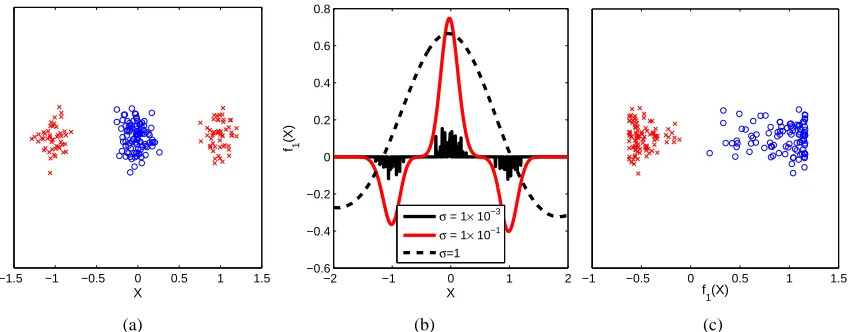
We illustrate this property with a simple toy example in Figure 1. Figure 1(a) plots our obser-vations, where one class has a bimodal distribution in feature X , with cluster centres at_±1. The second class has a single peak at the origin. The maximum singular vector f1(X)is shown in Figure

−1.5 −1 −0.5 0 0.5 1 1.5 X

(a)

−2 −1 0 1 2

−0.6 −0.4 −0.2 0 0.2 0.4 0.6 0.8

X

f1

(X)

σ = 1× 10−3

σ = 1× 10−1 σ=1

(b)

−1 −0.5 0 0.5 1 1.5

f

1(X) (c)

Figure 1: Maximum eigenfunction of the covrariance operator. Figure 1(a) contains the original data, where blue points have the label+1 and red points are labeled₋1. The feature of interest is plotted along the x-axis, and an irrelevant feature on the y-axis. Figure 1(b) contains the largest eigefunction of the covariance operator on the relevant feature alone, for three different kernel sizes: the smallest kernel shows overfitting, and the largest is too smooth. Figure 1(c) contains the mapped points for a “good” kernel choiceσ=0.1, illustrating a strong linear relation between the mapped points and the labels for this choice ofσ.

5.2.2 MULTICLASSCLASSIFICATION

Here we have a somewhat larger choice of options to contend with. Clearly the simplest kernel would be

l(y,y′) =cyδy,y′ where c_y>0. (18)

For cy=m−y1 we obtain a per-class normalization. Clearly, for n classes, the kernel matrix L can

be represented by the outer product of a rank-n matrix, where each row is given by cyie⊤yi, where ey

denotes the y-th unit vector inRn_{. Alternatively, we may adjust the inner product between classes}

to obtain

l(y,y′) =ψ

(y),ψ(y′)

(19)

whereψ(y) =ey

m my(m−my)−

z and z= ((m₋m1)−1, . . . ,(m−mn)−1)⊤.

5.2.3 REGRESSION

This is one of the situations where the advantages of using HSIC are clearly apparent: we are able to adjust our method to such situations simply by choosing appropriate kernels. Clearly, we could just use a linear kernel l(y,y′) =yy′which would select simple correlations between data and labels.

Another choice is to use an RBF kernel on the labels, such as

l(y,y′) =exp

−σ¯y−y′

2

. (20)

This will ensure that we capture arbitrary nonlinear dependence between x and y. The price is that in this case L will have full rank, hence computation of BAHSIC and FOHSIC are correspondingly more expensive.

6. Connections to Other Approaches

We now show that several feature selection criteria are special cases of BAHSIC by choosing appro-priate preprocessing of data and kernels. We will directly relate these criteria to the biased estimator HSIC0 in (4). Given the fact that HSIC0 converges to HSIC1with rate

O

(m−1)it follows that the

criteria are well related. Additionally we can infer from this that by using HSIC1these other criteria

could also be improved by correcting their bias. In summary BAHSIC is capable of finding and exploiting dependence of a much more general nature (for instance, dependence between data and labels with graph and string values).

6.1 Pearson Correlation

Pearson’s correlation is commonly used in microarray analysis (van’t Veer et al., 2002; Ein-Dor et al., 2006). It is defined as

Rj:=

1 m

m

∑

i=1

xi j−x¯j

sxj

yi−y¯

sy

where (21)

¯ xj=

1 m

m

∑

i=1

xi j and ¯y=

1 m

m

∑

i=1

yiand s2xj=

1 m

m

∑

i=1

(xi j−x¯j)2and s2y=

1 m

m

∑

i=1

(yi−y¯)2.

This means that all features are individually centered by ¯xj and scaled by their coordinate-wise

variance sxj as a preprocessing step. Performing those operations before applying a linear kernel

yields the equivalent HSIC0formulation:

tr KHLH=trXX⊤Hyy⊤H=

HX

⊤_Hy

2

(22)

=

d

∑

j=1 m

∑

i=1

xi j−x¯j

sxj

yi−y¯

sy !2

=

d

∑

j=1

R2_j. (23)

Hence HSIC1computes the sum of the squares of the Pearson Correlation (pc) coefficients. Since

6.2 Mean Difference and Its Variants

The difference between the means of the positive and negative classes at the jth feature,(x¯j+−x¯j−),

is useful for scoring individual features. With different normalization of the data and the labels, many variants can be derived. In our experiments we compare a number of these variants. For example, the centroid (lin) (Bedo et al., 2006), t-statistic (t), signal-to-noise ratio (snr), moderated t-score (m-t) and B-statistics (lods) (Smyth, 2004) all belong to this family. In the following we make those connections more explicit.

Centroid Bedo et al. (2006) use vj:=λx¯j+−(1−λ)x¯j−forλ∈(0,1)as the score for feature j.4

Features are subsequently selected according to the absolute valuev_j

. In experiments the

authors typically chooseλ=1 2.

Forλ=1

2 we can achieve the same goal by choosing Lii′ = yiyi′

m_yimy_i′ (yi,yi′∈ {±1}), in which

case HLH=L, since the label kernel matrix is already centered. Hence we have

tr KHLH=

m

∑

i,i′₌₁ yiyi′ myimyi′

x⊤_i xi′ =

d

∑

j=1 m

∑

i,i′₌₁

yiyi′x_{i j}x_i′_j myimyi′

!

=

d

∑

j=1

(x¯j+−x¯j−)2.

This proves that the centroid feature selector can be viewed as a special case of BAHSIC in the case ofλ=1

2. From our analysis we see that other values ofλamount to effectively rescaling

the patterns xi differently for different classes, which may lead to undesirable features being

selected.

t-Statistic The normalization for the jth feature is computed as

¯ sj=

"

s2_j+ m+

+s 2

j−

m₋

#1₂

. (24)

In this case we define the t-statistic for the jth feature via tj= (x¯j+−x¯j−)/s¯j.

Compared to the Pearson correlation, the key difference is that now we normalize each feature not by the overall sample standard deviation but rather by a value which takes each of the two classes separately into account.

Signal to noise ratio is yet another criterion to use in feature selection. The key idea is to normalize

each feature by ¯sj =sj++sj− instead. Subsequently the (x¯j+−x¯j−)/s¯j are used to score

features.

Moderated t-score is similar to t-statistic and is used for microarray analysis (Smyth, 2004). Its

normalization for the jth feature is derived via a Bayes approach as

˜ sj=

m ¯s2 j+m0s¯20

m+m0

where ¯sjis from (24), and ¯s0and m0are hyperparameters for the prior distribution on ¯sj(all ¯sj

are assumed to be iid). ¯s0and m0are estimated using information from all feature dimensions.

This effectively borrows information from the ensemble of features to aid with the scoring of an individual feature. More specifically, ¯s0and m0can be computed as (Smyth, 2004)

m0=2Γ′−1

1 d

d

∑

j=1

(zj−¯z)2−Γ′ m

2

!

, (25)

¯ s2₀=exp

¯z₋Γ

m

2

+Γm0

2

−ln

m 0

m

whereΓ(_·)is the gamma function,′denotes derivative, zj=ln(s¯2j)and ¯z= 1d∑ d

j=1zj.

B-statistic is the logarithm of the posterior odds (lods) that a feature is differentially expressed. L¨onnstedt and Speed (2002) and Smyth (2004) show that, for large number of features, B-statistic is given by

Bj=a+b˜t2j

where both a and b are constant (b>0), and ˜tjis the moderated-t statistic for the jth feature.

Here we see that Bj is monotonic increasing in ˜tj, and thus results in the same gene ranking

as the moderated-t statistic.

The reason why these connections work is that the signal-to-noise ratio, moderated t-statistic, and B-statistic are three variants of the t-test. They differ only in their respective denominators, and are thus special cases of HSIC0if we normalize the data accordingly.

6.3 Maximum Mean Discrepancy

For binary classification, an alternative criterion for selecting features is to check whether the dis-tributions Pr(x_|y=1)and Pr(x_|y=₋1)differ and subsequently pick those coordinates of the data which primarily contribute to the difference between the two distributions.

More specifically, we could use Maximum Mean Discrepancy (MMD) (Gretton et al., 2007a), which is a generalization of mean difference for Reproducing Kernel Hilbert Spaces, given by

MMD=_kE_x[φ_(x)|y=1]−E_x[φ_(x)|y=−1]k2

H.

A biased estimator of the above quantity can be obtained simply by replacing expectations by av-erages over a finite sample. We relate a biased estimator of MMD to HSIC0again by setting m−+1

as the labels for positive samples and₋m−₋1 for negative samples. If we apply a linear kernel on labels, L is automatically centered, that is, L1=0 and HLH=L. This yields

tr KHLH=tr KL (26)

= 1

m2₊

m+

∑

i,j

k(xi,xj) +

1 m2₋

m−

∑

i,j

k(xi,xj)−

2 m+m−

m+

∑

i m−

∑

j

k(xi,xj)

=

1 m+

m+

∑

i

φ(xi)−

1 m₋

m−

∑

j φ(xj)

2

H

.

The quantity in the last line is an estimator of MMD with bias

O

(m−1)(Gretton et al., 2007a). This implies that HSIC0and the biased estimator of MMD are identical up to a constant factor. Since the

bias of HSIC0is also

O

(m−1), this effectively show that scaled MMD and HSIC1converges to each

6.4 Kernel Target Alignment

Alternatively, one could use Kernel Target Alignment (KTA) (Cristianini et al., 2003) to test di-rectly whether there exists any correlation between data and labels. KTA has been used for feature selection in this context. Formally it is defined as tr(KL)/_kK_kkL_k, that is, as the normalized cosine between the kernel matrix and the label matrix.

The nonlinear dependence on K makes it somewhat hard to optimize for. Indeed, for compu-tational convenience the normalization is often omitted in practice (Neumann et al., 2005), which leaves us with tr KL, the corresponding estimator of MMD.5_{Note the key difference, though, that}

normalization of L according to label size does not occur. Nor does KTA take centering into ac-count. Both normalizations are rather important, in particular when dealing with data with very uneven distribution of classes and when using data that is highly collinear in feature space. On the other hand, whenever the sample sizes for both classes are approximately matched, such lack of normalization is negligible and we see that both criteria are similar.

Hence in some cases in binary classification, selecting features that maximizes HSIC also maxi-mizes MMD and KTA. Note that in general (multiclass, regression, or generic binary classification) this connection does not hold. Moreover, the use of HSIC offers uniform convergence bounds on the tails of the distribution of the estimators.

6.5 Shrunken Centroid

The shrunken centroid (pam) method (Tibshirani et al., 2002, 2003) performs feature ranking using the differences from the class centroids to the centroid of all the data, that is

(x¯j+−x¯j)2+ (x¯j−−x¯j)2,

as a criterion to determine the relevance of a given feature. It also scores each feature separately. To show that this criterion is related to HSIC we need to devise an appropriate map for the labels y. Consider the feature mapψ(y) withψ(1) = (m−₊1,0)⊤ _{andψ(−1) = (0,m}−1

− )⊤. Clearly, when

applying H to Y we obtain the following centered effective feature maps

¯

ψ(1) = (m−₊1₋m−1,₋m−1)and ¯ψ(₋1) = (₋m−1,m−₋1₋m−1).

Consequently we may express tr KHLH via

tr KHLH=

1 m+

m+

∑

i=1 xi−

1 m

m

∑

i=1 xi

2

+

1 m₋

m−

∑

i=1 xi−

1 m

m

∑

i=1 xi

2

(27)

=

d

∑

j=1 



1 m+

m+

∑

i=1

xi j−

1 m

m

∑

i=1

xi j !2

+ 1

m₋

m−

∑

i=1

xi j−

1 m

m

∑

i=1

xi j !2

 (28)

=

d

∑

j=1

(x¯j+−x¯j)2+ (x¯j−−x¯j)2

.

5. The denominator provides a trivial constraint in the case where the features are individually normalized to unit norm for a linear kernel, since in this casekKk=d: that is, the norm of the kernel matrix scales with the dimensionality d