Linear Regression With Random Projections

Linear Regression With Random Projections

Odalric-Ambrym Maillard [email protected]

R´emi Munos [email protected]

INRIA Lille Nord Europe SequeL Project

40 avenue Halley

59650 Villeneuve d’Ascq, France

Editor:Sanjoy Dasgupta

Abstract

We investigate a method for regression that makes use of a randomly generated subspaceGP⊂F (of finite dimensionP) of a given large (possibly infinite) dimensional function spaceF, for ex-ample,L2([0,1]d_{;R). GPis defined as the span ofPrandom features that are linear combinations} of a basis functions ofF weighted by random Gaussian i.i.d. coefficients. We show practical mo-tivation for the use of this approach, detail the link that this random projections method share with RKHS and Gaussian objects theory and prove, both in deterministic and random design, approx-imation error bounds when searching for the best regression function inGPrather than inF, and derive excess risk bounds for a specific regression algorithm (least squares regression inGP). This paper stresses the motivation to study such methods, thus the analysis developed is kept simple for explanations purpose and leaves room for future developments.

Keywords: regression, random matrices, dimension reduction

1. Introduction

We consider a standard regression problem. Thus let us introduce

X

an input space, and

Y

=Rthe

real line. We denote by

P

an unknown probability distribution over the product space

Z

=

X

×R

and by

P

X its first marginal, that is, d

P

X(x) =

Z

R

P

(x,dy). In order for this quantity to be well

defined we assume that

X

is a Polish space (i.e., metric, complete, separable), see Dudley (1989,

Th. 10.2.2). Finally, let L2,PX(

X

;R) be the space of real-valued functions on

X

that are squared

integrable with respect to (w.r.t.)

P

X, equipped with the quadratic norm

kf_kPX

def

=

r_Z

X f 2_(x)dP

X(x).

In this paper, we consider that

P

has some structure corresponding to a model of regression with

random design; there exists a (unknown) function f⋆:

X

_→R such that if(xn,yn)n6N ∈

X

×Rare

independently and identically distributed (i.i.d.) according to

P

, then one can write

yn= f⋆(xn) +ηn,

whereηnis a centered noise, independent from

P

X, introduced for notational convenience. In terms

Let

F

⊂L2,PX(

X

;R)be some given class of functions. The goal of the statistician is to build,

from the observations only, a regression function bf_∈

F

that is closed to the so-called target function

f⋆, in the sense that it has a low excess riskR(f)₋R(f⋆), where the risk of any f _∈L2,PX(

X

;R)is

defined as

R(f) def=

Z

X×R

(y₋f(x))2d

P

(x,y).

Similarly, we introduce the empirical risk of a function f to be

RN(f) def

= 1 N

N

∑

n=1

[yn−f(xn)]2,

and we define the empirical norm of f as_kf_kN

def

=

s

1 N

N

∑

n=1

f(xn)2.

Function spaces and penalization. In this paper, we consider that

F

is an infinite dimensional

space that is generated by the span over a denumerable family of functions_{ϕi}i>1ofL2,PX(

X

;R):

We call the_{ϕi}i>1theinitial featuresand thus refer to

F

as to the initial feature space:

F

def=nfα(x)def=

∑

i>1

αiϕi(x),kαk<∞

o

.

Examples of initial features include Fourier basis, multi-resolution basis such as wavelets, and also less explicit features coming from a preliminary dictionary learning process.

In the sequel, for the sake of simplicity we focus our attention to the case when the target

function f⋆= fα⋆ belongs to the space

F

, in which case the excess risk of a function f can be

written as R(f)₋R(f⋆) =_kf₋f⋆_kPX.Since

F

is an infinite dimensional space, empirical risk

minimization in

F

defined by argmin

f∈F

RN(f)is certainly subject to overfitting. Traditional methods

to circumvent this problem consider penalization techniques, that is, one searches for a function that satisfies

b

f =arg min

f∈FRN(f) +pen(f),

where typical examples of penalization include pen(f) =λ_kf_kpp for p=1 or 2, whereλis a

pa-rameter and usual choices for the norm areℓ2 (ridge-regression: Tikhonov 1963) andℓ1(LASSO:

Tibshirani 1994).

Motivation.In this paper we follow a complementary approach introduced in Maillard and Munos (2009) for finite dimensional space, called Compressed Least Squares Regression, and extended in

Maillard and Munos (2010), which considers generatingrandomlya space

G

P∈

F

of finite

dimen-sionPand then returning an empirical estimate in

G

P. The empirical risk minimizer in

G

P, that is,

arg ming∈GPRN(g)is a natural candidate, but other choices of estimates are possible, based on

tra-ditional literature on regression whenP<N (penalization, projection, PAC-Bayesian estimates...).

The generation of the space

G

P makes use of random matrices, that have already demonstrated

their benefit in different settings (see for instance Zhao and Zhang 2009 about spectral clustering or Dasgupta and Freund 2008 about manifold learning).

for the proposed method, and also by providing links to other standards approaches, in order to encourage research in that direction, which, as showed in the next section, has already been used in several applications.

Outline of the paper. In Section 2, we quickly present the method and give practical motivation for investigating this approach. In Section 3, we give a short overview of Gaussian objects theory

(Section 3.1), which enables us to show how to relate the choice of the initial features_{ϕi}i>1to the

construction of standard function spaces via Gaussian objects (Section 3.2), and we finally state a useful version of the Johnson-Lindenstrauss Lemma for our setting (Section 3.3).

In Section 4, we describe a typical algorithm (Section 4.1), and then provide some quick survey of classical results in regression while discussing the validity of their assumptions in our setting (Section 4.2). Then our main results are stated in Section 4.3, where we provide bounds on

approxi-mation error of the random space

G

Pin the framework of regression with deterministic and random

designs, and in Section 4.4, where we derive excess risk bounds for a specific estimate.

Section 5 provides some discussion about existing results and finally appendix A contains the proofs of our results.

2. Summary Of The Random Projection Method

From now on, we assume that the set of features_{ϕi}i>1are continuous and satisfy the assumption

that,

sup

x∈Xk

ϕ(x)_k2_{<∞,whereϕ(x)}def_{= (ϕ}

i(x))i>1∈ℓ2andkϕ(x)k2 def=

∑

i>1

ϕi(x)2.

Let us introduce a set of P random features(ψp)16p6P defined as linear combinations of the

initial features_{ϕi}1>1weighted by random coefficients:

ψp(x)def=

∑

i>1

Ap,iϕi(x), for 16p6P, (1)

where the (infinitely many) coefficientsAp,iare drawn i.i.d. from a centered distribution (e.g.,

Gaus-sian) with variance 1/P. Then let us define

G

P to be the (random) vector space spanned by those

features, that is,

G

P def

=ng_β(x)def=

P

∑

p=1

βpψp(x),β∈RP

o

.

In the sequel,

P

G will refer to the law of the Gaussian variables,

P

ηto the law of the observation

noise and

P

Y to the law of the observations. Remember also that

P

X refers to the law of the inputs.

One may naturally wish to build an estimateg_bβin the linear space

G

P. For instance in the case of

deterministic design, if we consider the ordinary least squares estimate, that is,

b

β=arg min_β∈RPR_N(g_β), then we can derive the following result (see Section 4.4 for a similar result

with random design):

that on this event, the excess risk of the least squares estimate g_bβis bounded as

kg_bβ−f⋆_k2_N612 log(8N/δ)

P kα

⋆_k21

N

N

∑

n=1

kϕ(xn)k2+κB2

P+log(2/δ)

N , (2)

for some numerical constantκ>0.

Example: Let us consider as an example the features_{ϕi}i>1to be a set of functions defined by

rescaling and translation of a mother one-dimensional hat function (illustrated in Figure 1, middle column) and defined precisely in paragraph 3.2.2. Then in this case we can show that

kα⋆_k21

N

N

∑

n=1

kϕ(xn)k26

1 2kf

⋆

k2H1,

where H1=H1([0,1]) is the Sobolev space of order 1. Thus we deduce that the excess risk is

bounded as_kg_bβ−f⋆_k2_N=O(Bkf⋆kH_√1log(N/δ)

N )forPof the order

√ N.

Similarly, the analysis given in paragraph 3.2.1 below shows that when the features_{ϕi}i>1are

wavelets rescaled by a factor σi =σj,l =2−js for some real number s>1/2, where j,l are the

scale and position index corresponding to theith element of the family, and that the mother wavelet

enables to generate the Besov space

B

s,2,2([0,1])(see paragraph 3.2.1), then for some constantc, it

holds that

kα⋆_k21

N

N

∑

n=1

kϕ(xn)k26

c 1₋2−2s+1kf

⋆_k2 s,2,2.

Thus the excess risk in this case is bounded as_kg_bβ−f⋆_k2_N=O(Bkf⋆ks,2,2log(N/δ) √

N ).

2.1 Comments

The second term in the bound (2) is a usual estimation error term in regression, while the first term

comes from the additional approximation error of the space

G

Pw.r.t.

F

. It involves the norm of the

parameterα⋆_{, and also the normkϕ(x)kat the sample points.}

The nice aspects of this result:

• The weak dependency of this bound with the dimension of the initial space

F

. This appears

implicitly in the termskα⋆_k2_and 1

N∑ N

n=1kϕ(xn)k2, and we will show that for a large class of

function spaces, these terms can be bounded by a function of the norm of f⋆only.

• The result does not require any specific smoothness assumptions on the initial features_{ϕi}i>1;

by optimizing overP, we get a rate of orderN−1/2that corresponds to theminimaxrates under

such assumptions up to logarithmic factors.

• Because the choice of the subspace

G

Pwithin which we perform the least-squares estimate is

random, we avoid (with high probability) degenerated situations where the target function f⋆

cannot be well approximated with functions in

G

P. Indeed, in methods that consider a given

deterministic finite-dimensional subspace

G

of the big space

F

(such as linear approximation

infg∈GPkf

⋆_−gk

Nis large. On the other hand when we use the random projection method, the

random choice of

G

Pimplies that for any f⋆∈

F

, the approximation error infg_∈GPkf

⋆_−gk

N

can be controlled (by the first term of the bound (2)) in high probability. See section 5.2 for an illustration of this property. Thus the results we obtain is able to compete with non-linear approximation (Barron et al., 2008) or kernel ridge regression (Caponnetto and De Vito, 2007).

• In terms of numerical complexity, this approach is more efficient than non-linear regression

and kernel ridge regression. Indeed, once the random space has been generated, we simply solve a least squares estimate in a low-dimensional space. The computation of the Gram matrix involves performing random projections (which can be computed efficiently for several

choices of the random coefficients Ap,i, see Liberty et al. 2008; Ailon and Chazelle 2006;

Sarlos 2006 and many other references therein). Numerical aspects of the algorithms are described in Section 5.4.

Possible improvements. As mentioned previously we do not make specific assumptions about

the initial features_{ϕi}i>1. However, considering smoothness assumptions on the features would

enable to derive a better approximation error term (first term of the bound (2)); typically with a

Sobolev assumption or orders, we would get a term of orderP−2sinstead ofP−1. For simplicity of

the presentation, we do not consider such assumptions here and report the general results only.

The log(N) factor may be seen as unwanted and one would like to remove it. However, this

term comes from a variant of the Johnson-Lindenstrauss lemma combined with a union bound, and

it seems difficult to remove it, unless the dimension of

F

is small (e.g., we can then use covers) but

this case is not interesting for our purpose.

Possible extensions of the random projection method. It seems natural to consider other construc-tions than the use of i.i.d. Gaussian random coefficients. For instance we may consider Gaussian

variables with varianceσ2

i/Pdifferent for eachiinstead of homeoscedastic variables, which is

ac-tually equivalent to considering the features_{ϕ′_i}i>1withϕ′i=σiϕiinstead.

Although in the paper we develop results using Gaussian random variables, such method will essentially work similarly for matrices with sub-Gaussian entries as well.

A more important modification of the method would be to consider, like for data-driven

pe-nalization techniques, a data-dependent construction of the random space

G

P, that is, using a

data-driven distribution for the random variable Ap,i instead of a Gaussian distribution. However the

analysis developed in this paperwill notwork for such modification, due to the fact we longer have

independent variables, and thus a different analysis is required.

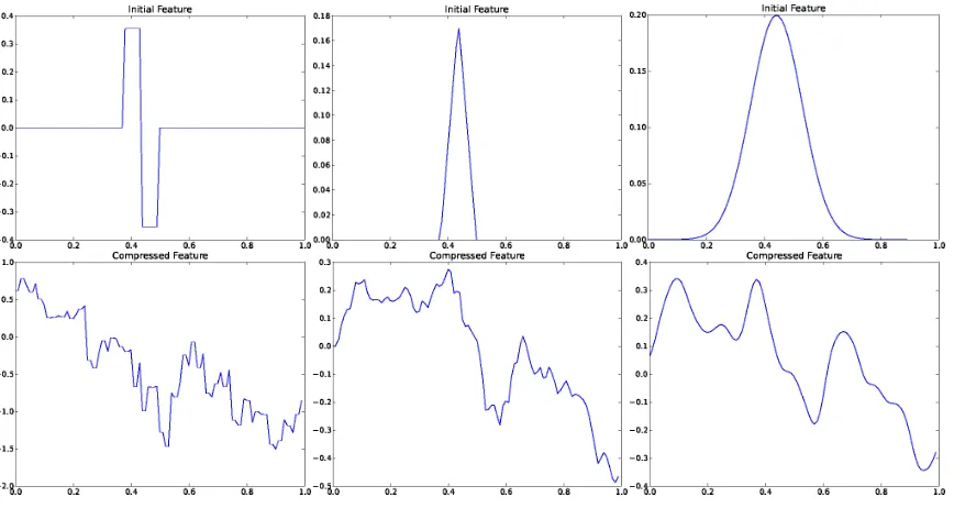
Illustration. In order to illustrate the method, we show in figure 1 three examples of initial

features _{ϕi} (top row) and random features{ψp} (bottom row). The first family of features is

the basis of wavelet Haar functions. The second one consists of multi-resolution hat functions (see paragraph 3.2.2) and the last one shows multi-resolution Gaussian functions. For example, in the case of multi-resolution hat functions (middle column), the corresponding random features are Brownian motions. The linear regression with random projections approach described here simply consists in performing least-squares regression using the set of randomly generated features

Figure 1: Three representative of initial featuresϕ(top row) and a sample of a corresponding

ran-dom featureψ(bottom row). The initial set of features are (respectively) Haar functions

(left), multi-resolution hat functions (middle) and multi-resolution Gaussian functions (right).

2.2 Motivation From Practice

We conclude this introduction with some additional motivation to study such objects coming from practical applications. Let us remind that the use of random projections is well-known in many domains and applications, with different names according to the corresponding field, and that the corresponding random objects are widely studied and used. Our contribution is to provide an anal-ysis of this method in a regression setting.

For instance, in Sutton and Whitehead (1993) the authors mentioned such constructions under

the namerandom representationas a tool for performing value function approximation in practical

implementations of reinforcement learning algorithms, and provided experiments demonstrating the benefit of such methods. They also pointed out that such representations were already used in 1962 in Rosenblatt’s perceptron as a preprocessing layer. See also Sutton (1996) for other comments concerning the practical benefit of “random collapsing” methods.

Another example is in image processing, when the initial features are chosen to be a wavelet

(rescaled) system, in which case the corresponding random features_{ψp}16p6Pare special cases of

random wavelet series, objects that are well studied in signal processing and mathematical physics (see Aubry and Jaffard 2002; Durand 2008 for a study of the law of the spectrum of singularities of these series).

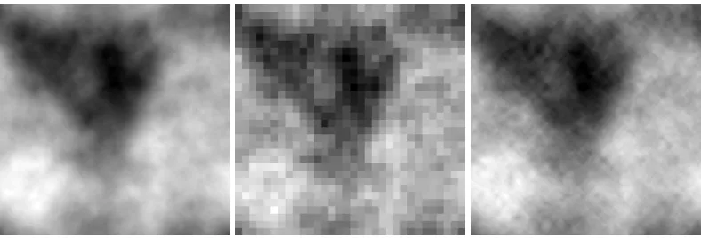
Figure 2: Example of an initial large texture (left), subsampled (middle), and possible recovery using regression with random projections (right)

and Benassi (2001). In their paper, the authors show that with the appropriate choice of the wavelet

functions and when using rescaling coefficients of the formσj,l=2−jswith scale indexjan position

index l(see paragraph 3.2.1), where sis not a constant but is now a function of jandl, we can

generate fractional Brownian motions, multi-scale fractional Brownian motions, and more generally what is called intermittent locally self-similar Gaussian processes.

In particular, for image texture generation they introduce a class of functions called morphlets

that enables to perform approximations of intermittent locally self-similar Gaussian processes. These approximations are both numerically very efficient and have visually imperceptible differ-ences to the targeted images, which make them very suitable for texture generation. The authors

also allow other distributions than the Gaussian for the random variablesξ (which thus does not

fit the theory presented here), and use this additional flexibility to produce an impressive texture generator.

Figure 2 illustrates an example performed on some simple texture model1 where an image of

size 512_×512 is generated (two-dimensional Brownian sheet with Hurst indexH=1.1) (left) and

then subsampled at 32_×32 (middle), which provides the data samples for generating a regression

function (right) using random features (generated from the symlets as initial features, in the simplest

model whensis constant).

3. Gaussian Objects

We now describe some tools of Gaussian object theory that would be useful in later analysis of

the method. Each random featureψpbuilt from Equation (1), when the coefficients are Gaussian,

qualifies as a Gaussian object. It is thus natural to study some important features of Gaussian objects.

3.1 Reminder of Gaussian Objects Theory

In all this section,

S

will refer to a vector space,

S

′ _{to its topological dual, and(·,·)to its duality}

product. The reader mostly interested in application of the random projection method may skip this section and directly go to Subsection 3.2 that provides examples of function spaces together with explicit construction of the abstract objects considered here.

Definition 2 (Gaussian objects) A random variable W _∈

S

is called a Gaussian object if for all

ν_∈

S

′_{,(ν,W)is a Gaussian (real-valued) variable. We further call any a∈}

_S

_{to be anexpectation} of W if

∀ν_∈

S

′,_E(ν,W) = (ν,a)<∞,

and any K:

S

′→

S

to be acovariance operatorof W if

∀ν,ν′_∈

S

′,Cov((ν,W)(ν′,W)) = (ν,Kν′)<∞,

where Cov refers to the correlation between two real-valued random variables.

Whenever there exist such a and K, we say that W follows the law

N

(a,K). Moreover, W is called a centered Gaussian object if a=0.

Kernel space. We only provide a brief introduction to this notion and refer the interested reader to Lifshits (1995) or Janson (1997) for refinements.

Let I′ :

S

′ →L2(

S

,

N

(0,K)) be the canonical injection from the space of continuous linear

functionals

S

′_{to the space of measurable linear functionals}

L2(

S

;R,

N

(0,K)) =

n

z:

S

→R,EW_∼N(0,K)|z(W)|2<∞ o

,

endowed with inner product_hz1,z2i=E(z1(W)z2(W)), that is, for anyν∈

S

′,I′is defined byI′(ν) =

(ν,_·). It belongs toL2(

S

;R,

N

(0,K))since by definition ofKwe have(ν,Kν) =E(ν,W)2<∞.

Then note that the space defined by

S

′

N def

=I′₍

_S

′_{), that is, the closure of the image of}

_S

′_byI′_{in the}

sense ofL2(

S

;R,

N

(0,K)), is a Hilbert space with inner product inherited fromL2(

S

;R,

N

(0,K)).

Now under the assumption thatI′is continuous (see Section 4.1 for practical conditions ensuring

that this is the case), we can define the adjointI:

S

_N′ →

S

ofI′, by duality. Indeed for anyµ_∈

S

′

andz_∈I′(

S

′_{), we have by definition that}

(µ,Iz) =I′µ,z_S′

N =EW((µ,W)z(W)),

from which we deduce by continuity thatIz=EW(W z(W)). For the sake of clarity, this specifies

for instance in the case when

S

=L2(

X

;R), for allx∈

X

as

(Iz)(x) =_EW(W(x)z(W)).

Now that the two injection mappingsI,I′have been defined, we are ready to provide the formal

(though slightly abstract) definition for our main object of interest:

A more practical way of dealing with kernels is given by the two following lemmas that we use extensively in Section 3.2. First, the kernel space can be built alternatively based on a separable

Hilbert space

H

as follows (Lifshits, 1995):

Lemma 4 (Construction of the Kernel space.) Let J:

H

→

S

be an injective linear mapping such that K=JJ′, where J′is the adjoint operator of J. Then the kernel space of

N

(0,K)is

K

=J(

H

),

endowed with inner product_hJh1,Jh2iH def

=_hh1,h2i_H.

We then conclude this section with the following Lemma from Lifshits (1995) that enables to

define the expansion of a Gaussian objectW.

Lemma 5 (Expansion of a Gaussian object) Let _{ϕi}i>1 be an orthonormal basis of

K

for the

inner product_h·,_·iK and{ξi i.i.d.

∼

N

(0,1)_}i>1. Then∑∞i=1ξiϕi is a Gaussian object following the

law

N

(0,K). It is called anexpansionfor

N

(0,K).

Note that from Lemma 4, one can build an orthonormal basis_{ϕi}i>1by defining, for alli>1,

ϕi=Jhiwhere{hi}i>1is an orthonormal basis of

H

andJ satisfies conditions of Lemma 4.

3.2 Interpretation of Some Function Spaces with Gaussian Objects Theory

In this section, we precise the link between Gaussian objects theory and reproducing kernel Hilbert spaces (RKHS) in order to provide more intuition about such objects. Indeed in many cases, the kernel space of a Gaussian object is a RKHS. Note, however, that in general, depending on the Gaussian object we consider, the former space may also be a more general space for instance when the Hilbert assumption is dropped (see Canu et al. 2002 about RKS). Therefore, there is no one-to-one correspondence between RKHS and kernel spaces of Gaussian objects and it is worth explaining when the two notions coincide. More importantly, this section shows various examples of classical

function spaces, related to the construction of the space

G

P for different choices of initial features

{ϕi}i>1, and that can be useful for applications.

3.2.1 GAUSSIANOBJECTS WITH ASUPPORTINGHILBERTSPACE

In this subsection only, we make the assumption that

S

=

H

is a Hilbert space and we introduce

{ei}i>1an orthonormal basis of

H

. Let us now considerξi∼

N

(0,1)i.i.d., and positive coefficients

σi>0 such that∑iσ2i <∞. Since∑iσ2i <∞, the Gaussian objectW=∑iξiσieiis well defined and

our goal is to identify the kernel of the law ofW.

To this aim we first identify the functionI′. Since

S

is a Hilbert space, then its dual is

S

′=

S

,

thus we consider f=∑iciei∈

S

′for somec∈ℓ2. For such an f, we deduce by the previous section

that the injection mapping is given by(I′_{f)(g) =∑}

ici(g,ei), and that we also have

kI′f_k2_S′

N =E (I

′_f,W)2₌

E

∑

i>1

σiξici2=

∑

i>1

σ2_ic2_i .

Now, since_kf_kS =kckℓ2, the continuity ofI′is insured by the assumption that∑iσ2i <∞, and

thusIis defined as in the previous section. Therefore, a function in the space

K

corresponding to f

is of the form∑iσiciei, and one can easily check that the kernel space of the law ofW is thus given

by

K

=nfc=

∑

i>1

ciei ;

∑

i>1

_ci

σi

endowed with inner product(fc,fd)K =∑i>1c_σid2i i

.

Reproducing Kernel Hilbert Spaces (RKHS).Note that if we now introduce the functions_{ϕi}i>1

defined byϕi

def

=σiei∈

H

, then we get

K

=nfα=

∑

i>1

αiϕi ;kαkl2 <∞

o

,

endowed with inner product(fα,fβ)K =hα,βil2. For instance, if we consider that

H

⊂L2,µ(

X

;R)

for some reference measureµ, and that _{ei}i>1 are orthonormal w.r.t. L2,µ(

X

;R), then

K

appears

to be a RKHS that can be made fully explicit; its kernel is defined byk(x,y) =∑∞_i=1σ2

iei(x)ei(y),

and _{σi}i>1 and {ei}i>1 are trivially the eigenvalues and eigenfunctions of the integral operator

Tk:L2,µ(

X

)→L2,µ(

X

)defined by(Tk(f))(x) = R

Xk(x,y)f(y)dµ(y).

Wavelet basis and Besov spaces. In this paragraph, we now apply the previous construction to

the case when the_{ei}i>1are chosen to be a wavelet basis of functions defined on

X

= [0,1]with

reference measureµbeing the Lebesgue measure. Letedenote the mother wavelet function, and let

us writeej,l theith element of the basis, with j∈Na scale index andl∈ {0, . . . ,2j−1}a position

index, where we re-index all families indexed byiwith the indice j,l. Let us define the coefficients

{σi}i>1to be exponentially decreasing with the scale index:

σj,l def

=2−js for all j>0 andl_{∈ {}0, . . . ,2j₋1_},

where we introduced some positive real numbers.

Now assume that for someq_∈N\ {0_}such thatq>s, the mother wavelet functionebelongs

to

C

q₍

_X

_{), the set of q-times continuously differentiable functions on}

_X

_{, and admits q vanishing}

moments. The reason to consider such case is that the (homogeneous) Besov space

B

s,2,2([0,1]d)

then admits the following known characterization (independent of the choice of the wavelets, see Frazier and Jawerth 1985; Bourdaud 1995):

B

s,2,2(

X

;µ) =

n

f _∈L2,µ(

X

);kfk2s,2,2 def

=

∞

∑

j=1

h

22js

2j₋₁

∑

l=0

|f,ej,l

|2i<∞o.

On the other hand, with the notations above, where in particularϕj,l =σj,lεj,l, we deduce that

the kernel space of the Gaussian object W =∑j,lξj,lϕj,l (that we call a Scrambled wavelet), is

simply the space

K

=nfα=

∑

j,l

αj,lϕj,l ;

∑

j,l

α2_j,l<∞o,

and a straightforward computation shows that_kα_k2

l2=kfαk

2

s,2,2, so that

K

=

B

s,2,2(

X

;µ). Moreover,

assuming that the mother wavelet is bounded by a constantλand has compact support[0,1], then

we have the property that is useful in view of our main Theorem

sup

x∈Xk

ϕ(x)_k26 λ 2

1₋2−2s+1.

Note that a similar construction applies to the case when the orthonormal basis_{ei}i>1is chosen

3.2.2 GAUSSIANOBJECTSDEFINED BY ACARLEMANEXPANSION

We now no longer assume that the supporting space

S

is a Hilbert space. In this case, it is still

possible to generate a Gaussian object with kernel space being a RKHS by resorting to Carleman operators.

A Carleman operator is a linear injective mappingJ:

H

7→

S

(where

H

is a Hilbert space) such

thatJ(h)(t) =RΓt(s)h(s)dswhere(Γt)t is a collection of functions of

H

. As shown for instance

in Canu et al. (2002); Saitoh (1988), there is a bijection between Carleman operators and the set of

RKHSs. In particular,J(

H

)is a RKHS.

A Gaussian object admittingJ(

H

)as a kernel space can be built as follows. By application of

Lemma 5, we have that

K

=J(

H

)endowed with the inner product_hJh1,Jh2iK

def

=_hh1,h2iH is the

kernel space of

N

(0,JJ′). Now, if we consider an orthonormal basis_{ei}i>1of

H

, an application

of Lemma 5 shows that the functions_{ϕi}i>1 defined byϕi

def

=J(ei)form an orthonormal basis of

J(

H

) and are such that the objectW =∑i>1ξiϕis first a well-defined Gaussian object and then

an expansion for the law

N

(0,JJ′). We call this expansion a Carleman expansion. Note that this

expansion is bottom-up whereas the Mercer expansion of a kernel via the spectral Theorem is top-down, see, for example, Zaanen (1960).

Cameron-Martin space. We apply as an example this construction to the case of the Brownian motion and the Cameron-Martin space.

Let

S

=

C

([0,1])be the space of continuous real-valued functions of the unit interval. Then

S

′ is the set of signed measures and we can define the dual product by (ν,f) =R_[0,1]f dν. It is

straightforward to check that the Brownian motion indexed by [0,1]is a Gaussian objectW _∈

S

,

witha_≡0 andKdefined by(Kν)(t) =R_[0,1]min(s,t)ν(ds).

Kernel space. We consider the Hilbert space

H

=L2([0,1])and define the mappingJ:

H

7→

S

by

(Jh)(t) =

Z

[0,t]h(s)ds;

simple computations show that (J′_{ν)(t) =ν([t,1]), K =JJ}′ _{and that J is a Carleman operator.}

Therefore, the kernel space

K

is equal toJ(L2([0,1])), or more explicitly

K

=k_∈H1([0,1]);k(0) =0 ,

whereH1([0,1])is the Sobolev space of order 1.

Expansion of the Brownian motion. We build a Carleman expansion for the Brownian motion

thanks to the Haar basis ofL2([0,1]), whose image byJdefines an orthonormal basis of

K

; the Haar

basis(e0,{ej,l}j,l∈N)is defined in a wavelet-way via a mother functione(x) =I[0,1/2[−I[1/2,1[and

father functione0(x) =I[0,1](x)with functions{ej,l}j,l_∈N defined for any scale j>1 and translation

index 06l62j₋1 by

ej,l(x) def

=2j/2e(2j_x−l).

An orthonormal basis of the kernel space of the Brownian motionW and an expansion ofW is thus

obtained by

W =

_∑

j,l>1

ξj,lϕj,l+ξ0ϕ0,

whereΛ(x) =xI[0,1/2[+ (1−x)I[1/2,1[ is the mother hat function.

Bounded energy. Note that the rescaling factor inside ϕj,l naturally appears as 2−j/2, and not

as 2j/2 _{as usually defined in wavelet-like transformations. Note also that since the support of the}

mother functionΛis[0,1], and also_kΛ_k∞61/2, then for any x∈[0,1]d, for all jthere exists at

most onel=l(x)such thatϕj,l(x)6=0, and we have the property that

kϕ(x)_k2 ₌

_∑

j>1

ϕ_j,l(x)(x)2 ₆

_∑

j>1

(2−j/2_kΛk ∞)2 6

1 2.

Remark 6 This construction can be extended to the dimension d>1in at least two ways. Consider the space

S

=

C

([0,1]d_{), and the Hilbert space}

_H

_=L

2([0,1]d). Then if we define J to be the volume

integral(Jh)(t) =R_[0,t]h(s)ds where[0,t]_⊂[0,1]d_{, this corresponds to the covariance operator}

de-fined by(Kν)(t) =R_[0,1]dΠd_i=1min(si,ti)ν(ds), that is, to the Brownian sheet defined by tensorization

of the Brownian motion. The corresponding kernel space in this case is thus

K

=J(L2_([0,1]d_)),

endowed with the norm _kf_kK =k ∂

d_f

∂x1...∂xdkL2([0,1]d). It corresponds to the Cameron-Martin space (Janson, 1997) of functions having a d-th order crossed (weak) derivative _∂x∂df

1...∂xd that belongs to L2([0,1]d_{), vanishing on the “left” boundary (edges containing0) of the unit d-dimensional cube.}

A second possible extension that is not detailed here would be to consider the isotropic Brownian sheet.

3.3 A Johnson-Lindenstrauss Lemma for Gaussian Objects

In this section, we derive a version of the Johnson-Lindenstrauss’ lemma that applies to the case of Gaussian objects.

The original Johnson-Lindenstrauss’ lemma can be stated as follows; its proof directly uses concentration inequalities (Cramer’s large deviation Theorem from 1938) and may be found, for example, in Achlioptas (2003).

Lemma 7 Let A be a P_×F matrix of i.i.d. Gaussian

N

(0,1/P)entries. Then for any vectorαin

RF, the random (with respect to the choice of the matrix A) variable_kAα_k2_{concentrates around its}

expectation_kα_k2_{when P is large: forε∈(0,1), we have}

PkAα_k2_>(1+ε)kαk2 _{6 e}−P(ε2_/4 −ε3_/6)

,

and PkAα_k2₆₍₁

−ε)_kα_k2 _{6 e}−P(ε2_/4−ε3_/6) .

Remark 8 Note the Gaussianity is not mandatory here, and this is also true for other distributions, such as:

• Rademacher distributions, that is, which takes values±1/√P with equal probability1/2,

• Distribution taking values_±p3/P with probability1/6and0with probability2/3.

What is very important is the scaling factor1/P appearing in the variance of

N

(0,1/P).

Lemma 9 Let{xn}n6Nbe N (deterministic) points of

X

. Let A:ℓ2(R)7→RPbe the operator defined

with i.i.d. Gaussian

N

(0,1/P)variables(Ai,p)i>1,p6P, such that for allα∈ℓ2(R), then

(Aα)p=

∑

i>1

αiAi,p.

Let us also defineψp=

∑

i>1

Ai,pϕi, fα=

∑

i>1

αiϕiand gβ= P

∑

p=1

βpψp.

Then, A is well-defined and for all P>1, for allε_∈(0,1), with probability larger than1₋ 4Ne−P(ε2/4−ε3/6)w.r.t. the Gaussian random variables,

kfα−gAαk2N6ε2kαk2

1 N

N

∑

n=1

kϕ(xn)k2,

where we recall that by assumption, for any x,ϕ(x)def= (ϕi(x))i>1is inℓ2.

This result is natural in view of concentration inequalities, since for all x_∈

X

, the

expecta-tion satisfiesEPG(gAα(x)) = fα(x)and the varianceVPG(gAα(x)) =

1 P(f

2

α(x) +kαk2kϕ(x)k2). See

Appendix A.1 for the full proof.

Note also that a natural idea in order to derive generalization bounds would be to derive a similar

result uniformly over

X

instead of a union bound over the samples. However, while such extension

would be possible for finite dimensional spaces

F

(by resorting to covers) these kind of results are

not possible in the general case, since

F

is typically big.

More intuition. Let us now provide some more intuition about when such a result is interesting.

In interesting situations described in Section 4 we consider a number of projectionsPlower than

the number of data samples N, typically P is of order√N. Thus, it may seem counter-intuitive

that we can approximate—at a set ofNpoints—a function fαthat lies in a high (possibly infinite)

dimensional space

F

by a functiongAαin a space

G

of dimensionP<N.

Of course in general this is not possible. To illustrate this case, let us consider that there is no

noise, assume that all points(xn)n6N belong to the unit sphere, and thatϕis the identity of

X

=RD.

Thus a target functionf is specified by someα_∈RD(whereDis assumed to be large, that is,D>N)

and the response values areyn= fα(xn) =αTxn. Writeyb∈RDthe estimategAαat the points, that is,

such thaty_bn=gAα(xn). In that case, the bound of Lemma 9 provides an average quadratic estimation

error _N1_ky_−by_k2of order log(N/δ) P ||α||

2_{, with probability 1}

−δ.

On the other hand the zero-value regressor has an estimation error of

1 Nkyk

2₌ 1

N

N

∑

n=1

(αTxn)2=αTSα, where S

def

= 1 N

N

∑

n=1

xnxTn ∈RD×D.

This shows that the result of Lemma 9 is essentially interesting when α

T_Sα

kα_k2 ≫

log(N/δ)

P , which

may not happen in certain cases: Indeed if we specifically choose xn=en∈RD, forn6N6D,

where(e1, . . . ,eD)denotes the Euclidean basis ofRD, then for such a choice, we have

αT_Sα

||α_||2 =

∑N_d=1α2 d

N∑Dd=1α2d 6 1

N 6

log(N/δ)

which means that the random projection method fails to recover a better solution than a trivial one.

The reason why it fails is that in that case the points _{xn}n6N lie in a subspace of RD of

high-dimension N, that is, such that the information at any set of points does not help us to predict the value at any other point. Essentially, what Lemma 9 tells us is that the random projection method

will work when the points_{xn}n6N lie in a vector subspace of smaller dimensiond0<N and that

the d0 corresponding coefficients of α contain most information about α (i.e., the other D−d0

coordinates are small). Let us illustrate this case by considering the case wherexn=e_1+(nmodd0)

for alln6N. In that case, we have (forNmultiple ofd0),

αT_Sα

||α_||2 =

∑d0

d=1α2d

d0∑Dd=1α2d ,

which is larger thanlog(_PN/δ)whenever the components_{αd}d>d0decrease fast andPis large enough,

in which case, the random projection method will work well.

Now introducing features, the condition says that the number of relevant features should be rela-tively small, in the sense that the parameter should mostly contain information at the corresponding coordinates, which is the case in many functional spaces, such as the Sobolev and Besov spaces

(for whichD=∞) described in Section 2 and Section 3.2.1, paragraph ”Wavelet basis and Besov

spaces”, for which _kα_k equals the norm of the function fα in the corresponding space. Thus a

”smooth” function fα(in the sense of having a low functional norm) has a low norm of the

param-eter_kα_k, and is thus well approximated with a small number of wavelets coefficients. Therefore,

Lemma 9 is interesting and the random projection method will work in such cases (i.e., the

addi-tional projection error is controlled by a term of order_kα_k2 log(N/δ)

P ).

4. Regression With Random Subspaces

In this section, we describe the construction of the random subspace

G

P⊂

F

defined as the span

of the random features _{ψp}p6P generated from the initial features {ϕi}i>1. This method was

originally described in Maillard and Munos (2009) for the case when

F

is of finite dimension, and

we extend it here to the non-obvious case of infinite dimensional spaces

F

, which relies on the fact

that the randomly generated features_{ψp}p6P are well-defined Gaussian objects.

The next subsection is devoted to the analysis of the approximation power of the random features space. We first give a survey of existing results on regression together with the standard hypothesis under which they hold in section 4.2, then we describe in section 4.4 an algorithm that builds the proposed regression function and provide excess risk bounds for this algorithm.

4.1 Construction of Random Subspaces

Assumption on initial features. In this paper we assume that the set of features_{ϕi}i>1are

con-tinuous and satisfy the assumption that,

sup

x∈Xk

ϕ(x)_k2<∞,where_kϕ(x)_k2 def=

∑

i>1

ϕi(x)2. (3)

Random features. The random subspace

G

P is generated by building a set of P random

fea-tures_{ψp}16p6Pdefined as linear combinations of the initial features{ϕi}1>1weighted by random

coefficients:

ψp(x)def=

∑

i>1

Ap,iϕi(x), for 16p6P,

where the (infinitely many) coefficientsAp,iare drawn i.i.d. from a centered distribution with

vari-ance 1/P. Here we explicitly choose a Gaussian distribution

N

(0,1/P). Such a definition of

the features ψp as an infinite sum of random variable is not obvious (this is an expansion of a

Gaussian object) and we refer to the Section 3 for elements of theory about Gaussian objects and Lemma 5 for the expansion of a Gaussian object. It is shown that under Assumption (3), the ran-dom features are well defined. Actually, they are ranran-dom samples of a centered Gaussian process

indexed by the space

X

with covariance structure given by_P1_hϕ(x),ϕ(x′)_i, where we use the notation

hu,v_idef=∑iuivifor two square-summable sequencesuandv. Indeed,EAp[ψp(x)] =0, and

CovAp(ψp(x),ψp(x′)) =EAp[ψp(x)ψp(x′)] = 1

P_i

∑

_>1ϕi(x)ϕi(x ′_{) =} 1

P

ϕ(x),ϕ(x′).

The continuity of each of the initial features_{ϕi}i>1guarantees that there exists a continuous version

of the processψpthat is thus a Gaussian process.

Random subspace. We finally define

G

P⊂

F

to be the (random) vector space spanned by those

features, that is,

G

P def

=ng_β(x)def=

P

∑

p=1

βpψp(x),β∈RP

o

.

We now want to compute a high probability bound on the excess risk of an estimator built using

the random space

G

P. To this aim, we first quickly review known results in regression and see

what kind of estimator can be considered and what results can be applied. Then we compute a high probability bound on the approximation error of the considered random space w.r.t. to initial space

F

. Finally, we combine both bounds in order to derive a bound on the excess risk of the proposed

estimate.

4.2 Reminder of Results on Regression

Short review of existing results. For the sake of completeness, we now review other existing results in regression that may or may not apply to our setting. Indeed it seems natural to apply

existing results for regression to the space

G

P. For that purpose, we focus on the randomness

coming from the data points only, and not from the Gaussian entries. We will thus consider in this

subsection only a space

G

that is the span over adeterministicset ofPfunctions_{ψp}p6P, and we

will write, for a convex subsetΘ_⊂RP_,

G

Θdef=gθ∈

G

;θ∈Θ .

Similarly, we writeg⋆def=argmin

g∈G

R(g)andg⋆_Θdef=argmin

g∈GΘ

R(g). Examples of well studied estimates

• gbolsdef=argmin_g∈GRN(g), the ordinary least-squares (ols) estimate.

• gbermdef=argmin_g∈GΘRN(g)the empirical risk minimizer (erm) that coincides with the ols when

Θ=RP.

• gbridgedef_=argmin

g∈GRN(g) +λkθk,gblasso def

=argmin_g∈GRN(g) +λkθk1.

We also introduce for conveniencegB, the truncation at level±Bof someg∈

G

, defined bygB(x)

def

=

TB[g(x)], whereTB(u) def

=

u if_|u_|6B,

Bsign(u) otherwise.

There are at least 9 different theorems that one may want to apply in our setting. Since those theorems hold under some assumptions, we list them now. Unfortunately, as we will see, these assumptions are usually slightly too strong to apply in our setting, and thus we will need to build our own analysis instead.

AssumptionsLet us list the following assumptions.

• Noise assumptions: (for some constantsB,B1,σ,ξ)

(N1)|Y|6B1,

(N2) supx∈XE(Y|X=x)6B,

(N3) supx∈XV(Y|X=x)6σ2,

(N4)∀k>3 supx∈XE(|Y|k|X=x)6σ2k!ξk−2.

• Moment assumptions: (for some constantsσ,a,M)

(M1)supx∈XE([Y−gΘ⋆(X)]2|X=x)6σ2,

(M2)supx∈XE(exp[a|Y−g⋆Θ(X)|]|X=x)6M,

(M3)∃g0∈

G

Θ supx_∈XE(exp[a|Y−g0(X)|]|X=x)6M.

• Function space assumptions for

G

: (for some constantD)

(G1) supg1,g2∈GΘkg1−g2k∞6D,

(G2)∃g0∈

G

Θ, known, such thatkg0−g⋆Θk∞6D.

• Dictionary assumptions:

(D1)L= max

16p6Pkψpk∞<∞,

(D2)L=supx∈Xkψ(x)k2<∞,

(D3)esssupkψ(X)k26L,

(D4)L= inf

{ψ′_p}p6P sup θ∈Rd_−{0}

k∑Pp=1θpψ′pk∞

kθ_k∞

<∞where the infimum is over all orthonormal

ba-sis of

G

w.r.t. toL2,PX(

X

;R).

• Orthogonality assumptions:

(O1){ψp}p6Pis an orthonormal basis of

G

w.r.t. toL2,PX(

X

;R),

(O2)det(Ψ)>0,whereΨ=E(ψ(X)ψ(X)T)is the Gram matrix.

• Parameter space assumptions:

(P1) supθ∈Θkθk∞<∞,

(P2)kθ⋆k16Swhereθ⋆is such thatgθ⋆=g⋆

ΘandSis known,

Theorem 10 (Gy¨orfi et al. 2002) Let Θ=_RP_{. Under assumption (N}

2) and(N3), the truncated

estimatorg_bL=TL(gbols)satisfies

ER(_bgL)−R(f(reg))68[R(g∗)−R(f(reg))] +κ

(σ2_∨B2_)Plog(N)

N ,

whereκis some numerical constant and f(reg)(x)def=E(Y_|X =x). Theorem 11 (Catoni 2004) Let Θ_⊂RP_{. Under assumption (M}

3), (G1) and (O2), there exists

constants C1,C2>0(depending only on a, M and D) such that with probability1−δ, provided that

n

g_∈

G

;RN(g)6RN(bgols) +C1

P N

o

⊂

G

Θ,

then the ordinary least squares estimate satisfies

R(g_bols)₋R(g⋆_Θ)6C2

P+log(δ−1_{) +log(}detΨb detΨ)

N ,

whereΨb =_N1∑Ni=1ψ(Xi)ψ(Xi)T is the empirical Gram matrix.

Theorem 12 (Audibert and Catoni 2010 from Alquier 2008) LetΘ=RP. Under assumption(N1)

and(G2), there exists a randomized estimateg that only depends on gb 0,L,C, such that for allδ>0,

with probability larger than1₋δw.r.t. all sources of randomness,

R(g)_{b −}R(g⋆)6κ(B2₁+D2)Plog(3ν −1

min) +log(log(N)δ−1)

N ,

whereκdoes not depend on P and N, andνminis the smallest eigenvalue ofΨ.

Theorem 13 (Koltchinskii 2006) LetΘ_⊂RP. Under assumption(N1),(D3)and(P3),gberm

satis-fies, for anyδ>0with probability higher than1₋δ,

R(g_berm)₋R(g_Θ⋆)6κ(B1+L)2

rank(Ψ) +log(δ−1₎

N ,

whereκis some constant.

Theorem 14 (Birg´e and Massart 1998) LetΘ_⊂RP. Under assumption(M3),(G1)and(D4), for

allδ>0with probability higher than1₋δ,

R(g_berm)₋R(g⋆_Θ)6κ(a−2+D2)Plog(2+ (L

2_{/N)∧(N/P)) +log(δ}−1₎

N ,

whereκis some constant depending only on M.

Theorem 15 (Tsybakov 2003) LetΘ=RP. Under assumption(N2),(N3)and(O1), the projection

estimate_bgpro jsatisfies

E(R(g_bpro j))₋R(g⋆)6(σ

2_+B2_)P

Theorem 16 (Caponnetto and De Vito 2007) Under assumption(M2)and(D2), for allδ>0for

λ=PL2log2(δ−1_)/N6ν

min, with probability higher than1−δ,

R(g_bridge)₋R(g⋆_Θ)6κ(a−2+λL

2_kθ⋆_k2_log2_(δ−1₎

νmin

)Plog

2_(δ−1₎

N ,

whereκis some constant depending only on M.

Theorem 17 (Alquier and Lounici 2011) LetΘ=_RP_{and define for allα∈(0,1)the priorπ} α(J) = α|J|

∑Ni=0αi

P

|J|

−1

for all J⊂2P_{. Under assumption(N}

2),(N3),(N4),(D1)and(P2), by settingλ= _2CN

where

Cdef=max_{64σ2+ (2B+L(2S+ 1 N))

2_{,64[ξ+2B+L(2S+} 1

N)]L(2S+ 1 N)},

the randomized aggregate estimatorg defined in Alquier and Lounici (2011) based on prior_b πα

satisfies, for anyδ>0with probability higher than1₋δ,

R(g)_{b −}R(g⋆_Θ)6CS

⋆_log((S+c)eNP

αS⋆ ) +log(2δ−1/(1−α))

N +

3L2

N2,

where S⋆=_kθ⋆_k

0.

Theorem 18 (Audibert and Catoni 2010) LetΘ_⊂RP_{. Under assumption(M}

1),(G1)and(P1)so

that one can define the uniform probability distribution overΘ, there exists a random estimatorg_b (drawn according to a Gibbs distributionbπ) that satisfies, with probability higher than1₋δw.r.t. all source of randomness,

R(g)_{b −}R(g⋆_Θ)6(2σ+D)216.6P+12.5 log(2δ−1)

N .

Note that Theorem 10 and Theorem 15 provide a result in expectation only, which is not enough for our purpose, since we need high probability bounds on the excess risk in order to be able to

handle the randomness of the space

G

P.

Assumptions satisfied by the random space

G

P

We now discuss the assumptions that are satisfied in our setting where

G

is a random space

G

P

built from the random features_{ψp}p6P, in terms of assumptions on the underlying initial space

F

.

• The noise assumptions(N)do not concern

G

.

• The moment assumptions(M)are not restrictive. By combining similar assumptions on

F

,

the results on approximation error of Section 4.3 can be shown to hold (with different con-stants).

• Assumptions(P)are generally too strong. For(P1), the reason is that there is no high

prob-ability link between_kAα_k∞andkαk for usual norms. Now even ifα⋆ is sparse or has low

l1-norm, this does not imply this is the case forβ⋆=argminβ∈RPR(g_β)orAα⋆in general, thus

(P2) cannot be assumed either. Finally(P3)may be assumed in some cases: Let us assume

that we know that_kα⋆_k

261. ThenkAα⋆k261+εwith high probability, thus it is enough to

consider the space

G

P(Θ)with parameter spaceΘ={β;kβk26(1+ε)}, and thusAα⋆∈Θ

• Assumptions(G)are strong assumptions. The reason is that it is difficult to relate the vector

coefficientβ⋆ or evenAα⋆to the vector coefficientα⋆ of f⋆= fα⋆ inl_∞norm. Thus even if

we know some f0close to f⋆inℓ∞-norm, this does not imply that we can build a functiong0

close tog⋆=gβ⋆.

• Assumptions(D)will not be valid a.s. w.r.t. the law of the Gaussian variables. The

assump-tions(D1)and(D4)are difficult to satisfy since they concernk.k∞. For assumption(D2)and

(D3), we have the property that for eachx,kψ(x)k22is close tokϕ(x)k22with high probability.

However, we need here a uniform result overx_∈

X

which seems difficult to get since the

space

F

is actually big (not of finite dimension).

• Assumptions(O), which are typically strong assumptions for specific featuresϕappear to be

almost satisfied. The reason is due to the covariance structure of the random features. Indeed

whatever the distribution

P

X (independent of

P

G), we have thathψp,ψqiconcentrates around

EPGhψp,ψqi=

1

Pk_i

∑

_>1ϕik

2 PXδp,q,

where δp,q is the Kronecker symbol between p andq. Thus the orthogonality assumption

is satisfied with high probability. Note that the knowledge of

P

X is still needed in order to

rescale the features and obtain orthonormality. Similar argument shows that(O2)is also valid.

As a consequence, only Theorems 10 and 15 would apply safely, but unfortunately these Theo-rems do not give results in high probability.

In the next two sections, we derive similar results but in high probability with assumptions that correspond to our setting. We provide a hand-made Theorem that makes use of the technique intro-duced in Gy¨orfi et al. (2002) and that can be applied without too restrictive assumptions, although not being optimal in terms of constant and logarithmic factors.

4.3 Approximation Power of Random Spaces

We assume from now on that we are in the case when f⋆= fα⋆∈

F

.

Theorem 19 (Approximation error with deterministic design) For all P>1, for allδ_∈(0,1) there exists an event of

P

G-probability higher than1−δsuch that on this event,

inf

g∈GPk

f⋆₋g_k2_N 612log(4N/δ)

P kα

⋆_k21

N

N

∑

n=1

kϕ(xn)k2.

Theorem 20 (Approximation error with random design) Under assumption(N2),

then for all P>1, for all δ_∈(0,1), the following bound holds with

P

G-probability higher than

1₋δ:

inf

g∈GPk

f⋆−TB(g)k2PX 6 25

kα⋆_k2_sup

xkϕ(x)k2

P

1+1

2log

Plog(8P/γ2_δ)

18γ2_δ

,

whereγdef= 1 Bkα

⋆_ksup

The result is not trivial because of the randomness of the space

G

P. Thus in order to keep

the explanation simple, the proof (detailed in the Appendix) makes use of Hoeffding’s Lemma only, which relies on the bounded assumption of the features (which can be seen either as a nice assumption, since it is simple and easy to check, or as a too strong assumption for some cases). Note that this result can be further refined by making use, for instance, of moment assumptions on the feature space instead.

4.4 Excess Risk of Random Spaces

In this section, we analyze the excess risk of the random projection method. Thus for a proposed

random estimateg, we are interested in bounding_b R(g)_{b −}R(f⋆)in high probability with respect to

any source of randomness.

4.4.1 REGRESSIONALGORITHM

From now on we consider the estimateg_bto be the least-squares estimateg_bβ∈

G

Pthat is the function

in

G

Pwith minimal empirical error, that is,

g_bβdef=arg min

gβ∈GP

RN(gβ), (4)

and that is the solution of a least-squares regression problem, that is,bβ=Ψ†_{Y ∈R}P _with

matrix-wise notations, whereY _∈RNis here the vector of observations (not to be confused with the random

variableY that shares the same notation),Ψis theN_×P-matrix composed of the elements:Ψn,p

def

=

ψp(xn), andΨ†is the Moore-Penrose pseudo-inverse2 ofΨ. The final prediction functiong(x)b is

the truncation (at level_±B) ofg_bβ, that is,g(x)_b def=TB[g_bβ(x)].

In the next subsection, we provide excess risk bounds w.r.t. f⋆in

G

P.

4.4.2 REGRESSION WITHDETERMINISTICDESIGN

Theorem 21 Under assumption(N1), then for all P>1, for allδ∈(0,1) there exists an event of

P

Y×

P

G-probability higher than1−δsuch that on this event, the excess risk of the estimator g_bβis

bounded as

kf⋆₋g_bβk2_N612 log(8N/δ)

P kα

⋆

k2_N1

N

∑

n=1

kϕ(xn)k2+κB21

P+log(2/δ)

N ,

for some numerical constantκ>0.

Note that from this theorem, we deduce (without further assumptions on the features_{ϕi}i>1)

that for instance for the choiceP=_log√_(NN_/δ)then

kf⋆₋g_bβk2_N6κ′h_kα⋆_k21

N

N

∑

n=1

kϕ(xn)k2

r

log(N/δ)

N +

log(1/δ)

N

i

,

for some positive constant κ′_{. Note also that whenever an upper-bound on the square terms}

kα⋆_k2 1 N∑

N

n=1kϕ(xn)k2 is known, this can be used in the definition of P in order to improve this

bound.

4.4.3 REGRESSION WITHRANDOMDESIGN

In the regression problem with random design, the analysis of the excess risk of a given method is not straightforward, since the assumptions to apply standard techniques may not be satisfied without further knowledge on the structure of the features. In a general case, we can use the techniques introduced in Gy¨orfi et al. (2002), which yields to the following (not optimal) result:

Theorem 22 Under assumption (N1) and (N2), provided that Nlog(N) > 4_P (thus whenever

min(N,P)>2), then with

P

G×

P

-probability at least1−δ,

R(TB(g_bβ))−R(f⋆) 6 κ

h_log(12N/δ)

P kα

⋆_k2_sup x∈Xk

ϕ(x)_k2

+max_{B2₁,B2_}P+Plog(N) +log(3/δ)

N

i

,

for some positive constantκ.

Let us now provide some intuition about the proof of this result. We first start by explaining what does not work. A natural idea in order to derive this result would be to consider the following decomposition:

R(TB(g_bβ))−R(f⋆)6[R(TB(g⋆B))−R(f⋆)] + [R(TB(g_bβ))−R(TB(g⋆B))],

whereg⋆_B∈argmin

g∈G

R(TB(g))−R(f⋆).

Indeed the first term is controlled on an eventΩG of high

P

G-probability by Theorem 20, and

sinceR(g_bβ)₋R(g⋆_B)6R(g_bβ)₋R(g⋆), the second term is controlled for each fixedωG ∈ΩG with

high

P

-probability by standard Theorems for regression, provided that we can relateR(TB(gbβ))−

R(TB(g⋆B))toR(gbβ)−R(g⋆B). Thus by doing the same careful analysis of the events involved, this

should lead to the desired result.

However, the difficulty lies first in ensuring that the conditions of application of standard

Theo-rems are satisfied with high

P

G-probability and then in relating the excess risk of the truncated

func-tion to that of the non-truncated ones, since it is not true in general thatR(TB(gbβ))−R(TB(g

⋆

B))6

R(g_bβ)₋R(g⋆

B). Thus we resort to a different decomposition in order to derive our results. The sketch

of proof of Theorem 22 actually consists in applying the following lemma.

Lemma 23 The following decomposition holds for all C>0

kTB(g_bβ)−f⋆k2PX 6 Ckf

⋆

−g_β˜k2_N+Ckg_β˜−g_bβk2_N

+sup

g∈G k

f⋆₋TB(g)k2PX−Ckf

⋆

−TB(g)k2N

,

where g_β˜ =Π_k.kN(f⋆,

G

) and gbβ=Πk.kN(Y,

G

) are the projections of the target function f⋆ and

observation Y onto the random linear space

G

with respect to the empirical norm_k._kN.

We then call the first term _kf⋆₋g_β˜k2N an approximation error term, the second kg_β˜−g_bβk2N a

noise error term and the third one sup_{g∈G k}f⋆₋TB(g)k_P2_X−Ckf⋆−TB(g)k2N

In order to prove Theorem 22, we then control each of these terms: We apply Lemma 19 to the first term, Lemma 24 below to the second term and finally Theorem 11.2 of Gy¨orfi et al. (2002) to

the last term withC=8, and the result follows by gathering all the bounds.

Let us now explain the contribution to each of the three terms in details.

Approximation error termThe first term,_kf⋆₋g_β˜k2N, is an approximation error term in empirical

norm, it contains the number of projections as well as the norm of the target function. This term plays the role of the approximation term that exists for regression with penalization by a factor

λ_kf_k2. This term is controlled by application of Theorem 19 conditionally on the random samples,

and then w.r.t. all source of randomness by independence of the Gaussian random variables with the random samples.

Noise error termThe second term,_kg_β˜−g_bβk2_N, is an error term due to the observation noiseη.

This term classically decreases at speed D_Nσ2 whereσ2 _{is the variance of the noise andDis related}

to the log entropy of the space of function

G

considered. Without any more assumption, we only

know that this is a linear space of dimensionP, so this term finally behaves like P_Nσ2, but note that

this dependency withPmay be improved depending on the knowledge about the functionsψ(for

instance, if

G

is included in a Sobolev space of orders, we would haveP1/2sinstead ofP).

Lemma 24 Under assumption (N1), then for each realization of the Gaussian variables, with

P

-probability higher than1₋δ, the following holds true:

kg_β˜−g_bβk2N66B21

1616P+200 log(6/δ) +log(3/δ)

N .

Note that we may consider different assumptions on the noise term. Here we considered only

that the noise is upper-bounded as_kη_k∞6B1, but another possible assumption is that the noise has

finite varianceσ2 _{or that the tail of the distribution of the noise behaves nicely, for example, that}

kη_kψα6B, whereψαis the Orlicz norm or orderα, withα=1 or 2. Estimation error term The third term, sup_g∈GP(_kf⋆₋TB(g)k2PX −Ckf

⋆_−T

B(g)k2N), is an

esti-mation of the error term due to finiteness of the data. This term also depends on the log entropy

of the space of functions, thus the same remark applies to the dependency withPas for the noise

error term. We bound the third term by applying Theorem 11.2 of Gy¨orfi et al. (2002) to the class of

functions

G

0_={f⋆_−T

B(g),g∈

G

P}, for fixed random Gaussian variables. Note that for all f∈

G

0,

kf_k∞62B. The precise result of Gy¨orfi et al. (2002) is the following :

Theorem 25 Let

F

be a class of functions f :Rd→Rbounded in absolute value by B. Letε>0. Then

P(sup

f_∈Fk

f_kPX−2kfkN>ε)63E(

N

(

√ 2

24ε,

F

,k.k2N))exp(− Nε2

288B2).

We now have the following lemma whose proof is given in the Appendix:

Lemma 26 Assuming that Nlog(N)>_P4, then for each realization of the Gaussian variables, with

P

-probability higher than1₋δ, the following holds true:

sup

g∈GP

kf⋆₋TB(g)k2PX−8kf

⋆

−TB(g)k2N6(24B)2

4 log(3/δ) +2Plog(N)

5. Discussion

In this section, we now provide more insights about the main results of this paper by reminding some closely related existing works, showing some numerical illustration of the method and discussing some numerical issues.

5.1 Non-linear Approximation

In the work of Barron et al. (2008), the authors provide excess risk bounds for greedy algorithms (i.e., in a non-linear approximation setting). The precise result they derive in their Theorem 3.1 is reported now, using the notations of section 4.2:

Theorem 27 (Barron et al. 2008) Consider spaces_{

G

P}P>1generated respectively by the span of

features_{ep}p6Pwith increasing dimension P (thusΘ=RPfor each P). For each

G

Pwe compute

a corresponding greedy empirical estimateg_bP∈

G

Pprovided by some algorithm (see Barron et al.,

2008), then we definePb=argmin_ky₋TB1bfPk

2 N+κ

Plog(N)

N for some constantκ, and finally define

b

g=TB1(bg_Pb), and fix some P0.

Under assumption(N1), there existsκ0depending only on B1and a where P0=xNaysuch that

ifκ>κ0, then for all P>0and for all functions gθin

G

P0, the estimatorg satisfiesb

ER(g)_{b −}R(f(reg))62[R(gθ)−R(f(reg))] +8k

θ_k2 1

P +C

PlogN

N ,

where the constant C only depends onκ, B1and a.

The bound is thus similar to that of Theorem 22 in Section 4.4. One difference is that this bound

contains thel1 norm of the coefficientsθ∗ while theℓ2 norm of the coefficientsα⋆ appears in our

setting. We leave as an open question to understand whether this difference is a consequence of the non-linear aspect of their approximation or if it results from the different assumptions made about the approximation spaces, in terms of rate of decrease of the coefficients.

The main difference is actually about the tractability of the proposed estimator, since the result of Theorem 27 relies on greedy estimation that is computationally heavy while on the other hand, random projection is cheap (see Subsection 5.4).

5.2 Adaptivity

Randomization enables to define approximation spaces such that the approximation error, either in expectation or in high probability on the choice of the random space, is controlled, whatever the

measure

P

that is used to assess the performance. This is specially interesting in the regression

setting where

P

is unknown. As mentioned in the introduction, because the choice of the subspace

G

Pwithin which we perform the least-squares estimate israndom, we avoid (with high probability)

degenerated situations where the target function f⋆cannot be well approximated with functions in

G

P. Indeed, in methods that consider a givendeterministicfinite-dimensional subspace

G

of the big

space

F

(such as linear approximation using a predefined set of wavelets), it is often possible to

find a target function f⋆such that infg∈GPkf

⋆_−gk

N is large, whereas using the random projection

method, the random choice of

G

Pimplies that for any f⋆∈

F

, the approximation error infg∈GPkf

⋆₋

g_kN can be controlled (by the first term of the bound (2)) in high probability. We now illustrate this