Learning to Construct Fast Signal Processing Implementations

(1)

Learning to Construct

Fast Signal Processing Implementations

Department of Computer Science Carnegie Mellon University Pittsburgh, PA 15213 USA

Editors: Carla E. Brodley and Andrea Danyluk

Abstract

A single signal processing algorithm can be represented by many mathematically equivalent formu-las. However, when these formulas are implemented in code and run on real machines, they have very different runtimes. Unfortunately, it is extremely difficult to model this broad performance range. Further, the space of formulas for real signal transforms is so large that it is impossible to search it exhaustively for fast implementations. We approach this search question as a control learning problem. We present a new method for learning to generate fast formulas, allowing us to intelligently search through only the most promising formulas. Our approach incorporates signal processing knowledge, hardware features, and formula performance data to learn to construct fast formulas. Our method learns from performance data for a few formulas of one size and then can construct formulas that will have the fastest runtimes possible across many sizes.

Keywords: Signal processing optimization, regression trees, decision trees, reinforcement learning

1. Introduction

Signal processing algorithms take as an input a signal, as a numerical dataset, and output a

trans-formation of the signal that highlights specific aspects of the dataset. Many signal processing

algo-rithms can be represented by a transformation matrix A which is multiplied by an input data vector

X to produce the desired output vector Y =A X (Rao and Yip, 1990). Na¨ıve implementations of

this matrix multiplication are too slow for large datasets or real time applications. However, the transformation matrices can be factored, allowing for faster implementations.

These factorizations can be represented by mathematical formulas and a single signal processing algorithm can be represented by many different, but mathematically equivalent, formulas (Auslan-der et al., 1996). Interestingly, when these formulas are implemented in code and executed, they have very different runtimes. The complexity of modern processors makes it difficult to analytically predict or model by hand the performance of formulas. Further, the differences between current processors lead to very different optimal formulas from machine to machine. Thus, a crucial prob-lem is finding the formula that impprob-lements the signal processing algorithm as efficiently as possible (Moura et al., 1998).

(2)

(Singer and Veloso, 2000), and we have also developed a stochastic evolutionary algorithm for find-ing fast implementations (Sfind-inger and Veloso, 2001). Other learnfind-ing researchers select the optimal algorithm from a few algorithms. For example, Brewer (1995) uses linear regression to predict runtimes for four different implementations, and Lagoudakis and Littman (2000) use reinforcement learning for selecting between two algorithms to solve sorting or order statistic selection problems. We consider thousands of different algorithms in this work.

Accurate prediction of runtimes (Singer and Veloso, 2000) still does not solve the problem of searching a very large number of formulas for a fast, or the fastest, one. At larger sizes, it is infeasible to just enumerate all possible formulas, let alone obtain predicted runtimes for all of them in order to choose the fastest. In this article we present a method that learns to generate formulas with fast runtimes. Out of the very large space of possible formulas, our method learns how to

control the generation of formulas to produce the formulas with the fastest runtimes. In fact, our

method is able to construct the fastest known formula within the first 100 formulas it generates, even in spaces with more than 50,000 different formulas. Remarkably, our new method can be trained on data from a particular sized transform and still construct fast formulas across many sizes. Thus, our method can generate fast formulas for many sizes, even when not a single formula of those sizes has been timed yet.

Our work relies on a number of important signal processing observations. We have success-fully integrated this domain knowledge into our learning algorithms. With these observations, we have designed a method for learning to accurately predict the runtime or number of cache misses incurred by a formula. Additionally, we can train these predictors using only data for formulas of one size while still accurately predicting the runtime or number of cache misses incurred by for-mulas of many different sizes. We then use these predictors along with a number of concepts from reinforcement learning to generate formulas that will have the fastest runtimes possible.

Section 2 describes some necessary background for understanding the rest of the article. Sec-tion 3 then describes our method for automatically learning a performance model. Then, SecSec-tion 4 describes our method for generating fast formulas. Finally, we conclude in Section 5.

2. Background

This section presents some signal processing background necessary for understanding the remainder of the article. For this work, we have focused on the Fast Fourier Transform (FFT) and the Walsh-Hadamard Transform (WHT).

2.1 The Transforms

The Discrete Fourier Transform (DFT) of a signal x of size s is the product DFT(s)·x where

DFT(s) = h

e2πikls

i

k,l=0,...,s−1

and k and l define the rows and columns of the matrix. For example,

DFT(21) =

1 1

1 −1

, DFT(22) =

   

1 1 1 1

1 i −1 −i

1 −1 1 −1

1 −i −1 i

(3)

The Walsh-Hadamard Transform of a signal x of size 2nis the product W HT(2n)·x where

W HT(2n) =

n

O

i=1

1 1

1 −1

,

and⊗is the tensor or Kronecker product (Beauchamp, 1984). If A is a m×m matrix and B a n×n

matrix, then A⊗B is the block matrix product

  

a_1,1B ··· a_1,mB

..

. . .. ...

am,1B ··· am,mB

  .

For example,

W HT(22) =

1 1

1 −1

⊗

1 1

1 −1

=    

1 1 1 1

1 −1 1 −1

1 1 −1 −1

1 −1 −1 1

   .

By calculating and combining smaller DFTs or WHTs appropriately, the structure in the trans-formation matrices can be leveraged to produce more efficient algorithms (for the DFT these are called Fast Fourier Transforms or FFTs).

The well known Cooley-Tukey factorization for the DFT (Cooley and Tukey, 1965) is:

DFT(rs) = (DFT(r)⊗Is)Tsrs(Ir⊗DFT(s))Lrsr

where Ik is the k×k identity matrix, Tsrsis the twiddle matrix (a sparse matrix), and Lrsr is a stride

permutation (another sparse matrix). We call this equation a “break down rule” as it specifies how

a DFT of size n=r×s can be factored into smaller DFTs of size r and s.

Let n=n1+···+nt with all of the nj being positive integers. Then,

W HT(2n) =

t

∏

i=1

(I₂n1+···+ni−1⊗W HT(2

ni)⊗_I

2ni+1+···+nt) .

These break down rules can then be recursively applied to each of these new smaller DFTs and WHTs. Thus, the FFT and the WHT can be implemented as any of a large number of different but mathematically equivalent formulas.

2.2 Split Trees

Any of these formulas for the FFT or WHT can be uniquely represented by a tree, which we call a

“split tree.” For example, suppose W HT(25)was factored as:

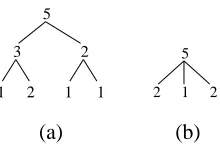
W HT(25) = [W HT(23)⊗I22][I₂3⊗W HT(22)]

= [{(W HT(21)⊗I₂2)(I₂1⊗W HT(22))} ⊗I₂2]

(4)

5

3 2

2

1 1 1

5 2 1 2

(a) (b)

Figure 1: Two different split trees for W HT(25).

The split tree corresponding to this final formula is shown in Figure 1(a). Each node in the split tree is labeled with the base two logarithm of the size of the WHT at that level. The children of a node indicate how the node’s WHT is recursively computed.

Implicit in the split tree is the stride at which nodes compute their respective DFTs or WHTs. A node’s stride determines how it accesses data from the input and output vectors. The exact nature of how nodes access data depending on their stride is not important for this article. However, it is important that stride can greatly impact the performance of the cache. Two nodes of the same size but that have different strides can have very different cache performance. Further, the stride of a node depends on its location in the split tree and the size of the nodes to its right.

2.3 WHT Timing Package

For the results with the WHT presented in this article we used a WHT package, (Johnson and P ¨uschel, 2000), which can implement in code and run WHT formulas passed to it. By using hard-ware performance counters, the package can count a number of different performance measures, including the number of cycles needed to execute the given formula or the number of cache misses incurred by the formula. The package can return performance measures for entire formulas or for

each node in the split tree. The WHT package allows leaves of the split trees to be sizes 21 to

28 which are implemented as unrolled straight-line code, while internal nodes are implemented as

recursive calls to their children.

We will be discussing the level 1 data cache which is the smallest and fastest memory cache closest to the CPU that contains data. Many processors also have a level 1 instruction cache to hold program instructions and a larger and slower level 2 cache closer to memory. The WHT package can specifically count the number of level 1 data cache misses. To simplify the discussion, we will often use the term “cache” in this article while we really mean “level 1 data cache.”

2.4 The SPIRAL System

For the results with the FFT presented in this article we used the SPIRAL system (Moura et al., 1998; P ¨uschel et al., 2002). Given a transform definition and break down rules for that transform, the SPIRAL system is able to construct any possible full factorization of a transform and implement that factorization in C or Fortran code. Further, the SPIRAL system provides methods to search over the different factorizations for a fast implementation.

(5)

performed an exhaustive search over all possible split trees of sizes 22 to 27, implementing them in unrolled, straight-line code. The system can then either continue factoring a transform using the Cooley-Tukey break down rule, implementing this in loops, or use one of these unrolled leaves (if the size is small enough).

The SPIRAL system has the ability to compile, run, and time the generated code. It can also use performance counters to keep track of the amount of runtime spent in computing different portions of the split tree. This allows the amount of runtime spent computing in each node in the split tree to be obtained. Unfortunately due to overhead, the timings become inaccurate for small sized nodes,

particularly those of size 21. To avoid this problem, we prevented the system from constructing split

trees with nodes of size 21, but instead had it use the leaves of sizes 22to 27.

2.5 Search Space

Even though we limited SPIRAL’s space of FFT implementations, there are still a large number of

possible FFT split trees. For example, at size 214 there are still 2,449 different split trees and at

size 218there are 70,376. There is also a very large number of possible formulas for a WHT of any

given size. W HT(2n)has on the order of θ((4+√8)n/n3/2)different possible formulas (Johnson

and P ¨uschel, 2000). For example, W HT(28)has 16,768 different split trees.

To aid in evaluating the performance of our algorithms with the WHT, we also limited the space of WHT formulas considered. We have observed that the fastest binary split trees are just as fast

as the fastest non-binary ones. However, there are still on the order of θ(5n/n3/2) binary split

trees (Johnson and P ¨uschel, 2000), making it infeasible to search through all binary split trees for transforms larger than the size of the cache. We have found that the fastest formulas never have

leaves of size 21 _{since it is beneficial to use unrolled code of larger sizes. Searching over all split}

trees with no leaves of size 21greatly reduces the search space, being feasible for formulas of sizes

larger than the cache. Unfortunately, it still becomes infeasible to exhaustively search over this

limited space for transforms much larger than 216. We have observed that the best split trees are

always rightmost (trees where every left child is a leaf). This limited space can be searched for larger sizes.

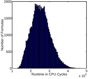
These different formulas have very different runtimes. Figure 2 shows a histogram of the

run-times of all DFT(218) formulas. There is about a factor of 4 difference in runtimes between the

fastest and slowest formulas. Further there are relatively few formulas that have the fastest times in comparison to those formulas that have about the average runtime.

1 2 3 4 5 x 108 0

500 1000 1500 2000

Runtime in CPU Cycles

Number of Formulas

(6)

3. Modeling Performance

In this section, we discuss our work in modeling performance for signal transforms. We begin in Section 3.1 with a number of key observations that we made for the WHT on a Pentium. These observations led us to develop methods for predicting cache misses for WHT leaves as discussed in Section 3.2. Next, Section 3.3 discusses our observations for the WHT on a Sun. These new obser-vations directed us to develop methods for predicting actual runtimes for WHT leaves as discussed in Section 3.4. Finally, Section 3.5 extends these methods for predicting runtimes for FFT leaves and internal nodes.

3.1 Pentium Observations

This section discusses several important observations that we made about the WHT that directed our research. Specifically, these observations were made on a Pentium III 450 MHz running Linux 2.2.5-15.

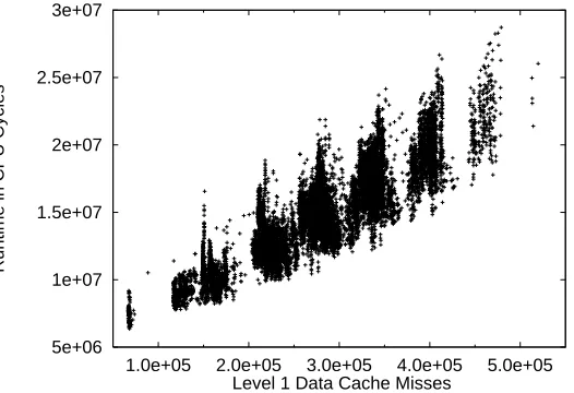
Figure 3 shows a scatter plot of runtimes versus level 1 data cache misses for all binary W HT(216)

split trees with no leaves of size 21. Each point in the scatter plot corresponds to a different WHT

formula. The placement of this point corresponds to that formula’s runtime and cache misses. The plot shows that while there is a complete spread of runtimes, there is a grouping of formulas with similar numbers of cache misses. Both runtimes and cache misses vary considerably differing by about a factor of 6 and 10 respectively from the smallest to the largest. Further, as the number of cache misses decreases so does the minimal and maximal runtimes for formulas with the same number of cache misses. The formula with the fastest runtime also has the minimal number of cache misses.

5e+06 1e+07 1.5e+07 2e+07 2.5e+07 3e+07

1.0e+05 2.0e+05 3.0e+05 4.0e+05 5.0e+05

Level 1 Data Cache Misses

Figure 3: Runtimes vs. cache misses for entire W HT(216)formulas on a Pentium.

(7)

The second key observation is that all of the runtime and cache misses occur in computing the leaves. The WHT package we are using (Johnson and P ¨uschel, 2000) implements leaf WHTs as unrolled, straight-line code. There is no work necessary to combine the leaf WHTs. The recursive calls to children from an internal node in the WHT package simply specify which portions of the input and output data vectors are to be operated on when calculating a smaller WHT. Additionally, the total runtime and number of cache misses of a formula is simply the sum of the runtime and cache misses at each of the leaves.

This observation allows us to consider simply modeling performance of individual leaves. The performance of an entire formula could then be predicted by summing up the individual predictions for the leaves.

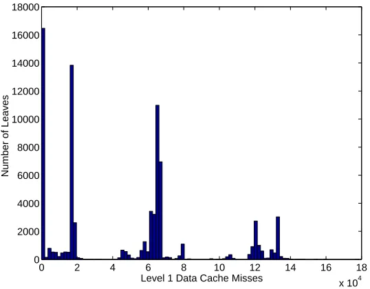
Figure 4 shows a histogram of the number of level 1 data cache misses incurred by leaves of all

binary W HT(216)split trees with no leaves of size 21. For all of the WHT formulas, the number

of cache misses incurred by each leaf was measured, and a histogram was generated over all these leaves. The spikes in the histogram show that the number of cache misses incurred by leaves takes on only a few possible values.

0 2 4 6 8 10 12 14 16 18

x 104 0

2000 4000 6000 8000 10000 12000 14000 16000 18000

Number of Leaves

Figure 4: Histogram of the number of cache misses incurred by leaves of W HT(216)formulas on

a Pentium.

Thus, it is not necessary to predict a real valued number of cache misses, but rather only to predict the correct group of cache misses out of only four groups. This observation indicates that simple classification algorithms can be used to predict cache misses for leaves instead of needing to use a function approximator.

(8)

• 0

• s/4

• s

• 2s or more.

These particular fractions correspond to particular features of the cache. To have no cache misses means that all of the data that the leaf needed was already in cache. To have as many cache misses as the size of the transform means that the leaf incurred one cache miss for each data item. On a Pentium machine, it is possible to have as many cache misses as one quarter of the size of the transform since a cache line holds exactly four data items. Further, it is possible to have more cache misses than data items, since a single data item may need to be accessed multiple times during a computation.

Thus, the number of level 1 data cache misses incurred by a leaf comes in only a few specific fractions of the size of the transform being computed. This suggests the possibility to learn across different sized WHTs by predicting cache misses in terms of fractions of the transform size.

In summary, we observed the following:

• For a given size, the WHT formula with the fastest runtime has the minimal number of level

1 data cache misses. So minimizing cache misses produces a group of formulas containing the fastest one.

• All of the computational time and cache misses occur in the leaves of the split trees. So

predicting leaf cache misses allows predicting for entire formulas.

• The number of level 1 data cache misses incurred by a leaf is only one of a few possible

values. So we can learn categories instead of real-valued numbers of cache misses.

• The number of level 1 data cache misses incurred by leaves are fractions of the transform

size. So learning may be able to generalize across different sizes.

3.2 Predicting WHT Leaf Cache Misses

Given the observations discussed in the previous section, we now turn to modeling level 1 data cache misses for WHT leaves. We discuss the features used for the leaves, then we present the learning algorithm, and finally we evaluate our approach.

3.2.1 FEATURES FORWHT LEAVES

To use standard machine learning methods to predict cache misses for WHT leaves, we need to describe the leaves with features. These features need to be able to distinguish leaves with different cache misses. The use of good features provides a source of domain knowledge about the WHT to our methods.

The features that we have decided to use came about from trying to model cache misses for leaves by hand. Trying to understand cache misses is difficult, and we were only able to understand a few simple cases by hand. However, after the attempt, we were able to write down a number of the features that we were considering.

(9)

each call. A leaf’s position in a split tree is also very important in determining its number of cache misses. The position of a leaf in a split determines the state of the cache when the leaf is called. However, it is not as easy to capture the position of a leaf in a split tree with numeric features as it is for the size of a leaf.

A leaf’s stride provides some information about its position in the split tree and describes how a leaf accesses its input and output data. Cache performance is clearly affected by the stride at which data is accessed. A leaf’s stride can be easily determined by its position in the split tree.

To provide more context of the position of a leaf in its split tree, the size and stride of the parent of the leaf can also be considered. These features indicate how much data the leaf will share with its siblings and how the data is laid out in memory.

Further, given a particular leaf l, the leaf p computed immediately before l gives information about l’s position in the tree. Specifically, this “previous” leaf p is the leaf just to the right of l along the fringe of the tree. However, the size and stride of the common parent between l and p (i.e., the first common node in the parent chains of both leaves) provide information about how much data is currently in the cache because of p and how it is laid out in memory. This is due to the fact that before l is called p has been called enough times so that it has accessed as much data as the size of the common parent. Further, p has accessed its data always at a multiple of the common parent’s stride, but at the appropriate initial offsets so that the total data brought in before l is called is exactly at the common parent’s stride. Thus, we use the size and stride of the “common parent” in our features and not that of the previous leaf.

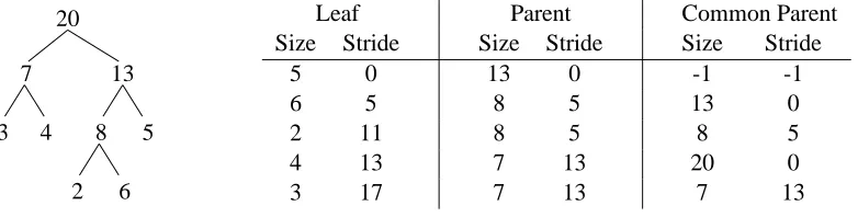
Figure 5 gives an example split tree along with the features for each of the leaves. Each line of the table corresponds to features for one leaf. The nodes in the split tree are labeled by the base two logarithms of their sizes (for convenience, no two nodes have the same size for this example). The features are actually given as base two logarithms of the sizes and strides. Further, the rightmost leaf has no common parent since no leaf is computed before it, and this is indicated by a “-1” value for the common parent features.

3 8 5

2 6

7

4

13

20 Leaf Parent Common Parent

Size Stride Size Stride Size Stride

5 0 13 0 -1 -1

6 5 8 5 13 0

2 11 8 5 8 5

4 13 7 13 20 0

3 17 7 13 7 13

Figure 5: Example leaf features for all of the leaves in the given split tree.

In summary, we use the following six features:

• Size and stride of the given leaf

• Size and stride of the parent of the given leaf

(10)

3.2.2 LEARNING ALGORITHM ANDTRAINING

Given these features for leaves, we can now use standard classification algorithms to learn to predict cache misses for WHT leaves. Our algorithm is as follows:

1. Run several different WHT formulas, collecting the number of level 1 data cache misses for each of the leaves.

2. Divide the number of cache misses by the size of the transform, and classify them as follows:

• near-zero, if less than 1/8

• near-quarter, if less than 1/2

• near-whole, if less than 3/2

• large, otherwise.

3. Describe each of the leaves with the features outlined in the previous subsection.

4. Train a classification algorithm to predict one of the four classes of cache misses given the leaf features.

While the classification algorithm predicts one of the four categories for any leaf, this can be translated back into actual cache misses. In a transform of size s, a leaf is predicted to have cache misses as follows:

• 0 cache misses, if near-zero is predicted;

• s/4 cache misses, if near-quarter is predicted;

• s cache misses, if near-whole is predicted;

• 2s cache misses, if large is predicted.

Further, the number of cache misses incurred by an entire formula can be predicted by summing over all the leaves.

We have specifically employed a C4.5 decision tree (Quinlan, 1992) as the classification algo-rithm in the experiments that follow, but other classification algoalgo-rithms should be usable. A decision tree was chosen as it allows rules that are somewhat human readable to be extracted and analyzed.

We trained a C4.5 decision tree on a random 10% of the leaves of all binary W HT(216) split

trees with no leaves of size 21. The actual number of level 1 data cache misses was collected for

these leaves by running their trees on a Pentium.

3.2.3 EVALUATION

There are several measures of interest for evaluating our learning algorithm. The simplest is to measure the accuracy at predicting the correct category of cache misses for leaves. Since we want to predict cache misses for entire trees, another measure is to evaluate the accuracy of using this predictor for entire formulas. Further, we are most interested in whether it accurately predicts the fastest formulas to have the fewest number of cache misses.

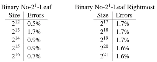
Table 1 evaluates the accuracy of our method at predicting the correct category of cache misses

(11)

formulas, using all of the formulas of the different limited formula spaces discussed in Section 2.5. The error rate shown is the percentage of the total number of leaves tested for which the decision tree predicted the wrong category. Clearly, there are very few errors, less than 2% in all cases shown. This is surprisingly good in that while training only on a small fraction of the total leaves of one size, the learned decision tree can accurately predict across a wide range of sizes.

Table 1: Error rates for predicting cache miss category incurred by leaves.

Binary No-21-Leaf Binary No-21-Leaf Rightmost

Size Errors

212 0.5%

213 1.7%

214 _0.9%

215 0.9%

216 0.7%

Size Errors

217 1.7%

218 1.7%

219 _1.7%

220 1.6%

221 1.6%

We used the same decision tree as in the previous experiment to predict cache misses for entire formulas. This was done by using the decision tree to predict a category for each leaf in the split tree. These categories were transformed into an actual number of cache misses as discussed in Section 3.2.2. Then the final prediction for the entire formula was made by summing the predicted number of cache misses incurred by each leaf within the split tree. We then calculated an average percentage error over a test set of formulas of a particular size as

1

|TestSet|_i_∈_TestSet

∑

|ai−pi| ai ,

where aiand piare the actual and predicted number of cache misses for formula i.

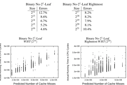
Table 2 shows the error on predicting cache misses for entire formulas. Tables 1 and 2 cannot be directly compared, since Table 1 shows the number of leaves for which an error is made, while Table 2 shows the average amount of error between the real and predicted number of cache misses. Further, we would expect a larger error when predicting the actual number of cache misses for an entire formula instead of just one of four categories for a single leaf.

Except for the extreme sizes shown in Table 2, the learned decision tree is able to predict within 10% of the real number of cache misses on average. This is surprisingly good especially considering that Figure 3 shows that there is about a factor of 10 difference in the number of cache misses incurred by different formulas of the same size. Further, this result is very good considering that this is predicting for entire formulas and not just leaves and that the decision tree was only trained

on data from formulas of size 216.

(12)

Table 2: Average percentage error for predicting cache misses for entire formulas.

Size Errors

212 12.7%

213 8.6%

214 6.7%

215 5.2%

216 4.6%

Size Errors

217 8.2%

218 8.2%

219 7.9%

220 8.1%

221 10.4%

Binary No-21_-Leaf _{Binary No-2}1_-Leaf

W HT(214₎ _{Rightmost W HT}₍₂20₎

1e+06 2e+06 3e+06 4e+06 5e+06

2.0e+04 4.0e+04 6.0e+04 8.0e+04 1.0e+05

Actual Running Time in CPU Cycles

Predicted Number of Cache Misses

1.5e+08 2e+08 2.5e+08 3e+08 3.5e+08 4e+08

2.0e+06 4.0e+06 6.0e+06

Actual Running Time in CPU Cycles

Predicted Number of Cache Misses

Figure 6: Runtime vs. predicted cache misses for entire formulas.

3.2.4 SUMMARY

In summary, we have presented a method for predicting a formula’s number of level 1 data cache misses by training a decision tree to predict a leaf’s number of cache misses to be one of only a few categories. We have also shown that this method produces very good results across a variety of sizes, including larger sizes, even when only trained on one particular size. This learned decision tree serves as a model of the cache performance of formulas.

3.3 Sun Observations

Given the excellent results achieved for predicting cache misses on a Pentium, we wished to see if the same methods would work on other architectures. In particular, we began by collecting data on a Sun UltraSparc IIi machine to see if the same observations described in Section 3.1 for the Pentium would carry over to the Sun.

Figure 7 shows a scatter plot of runtimes versus level 1 data cache misses for all binary rightmost

W HT(218₎_{split trees with no leaves of size 2}1_{. Unlike on the Pentium, the fastest formula on the}

Sun does not also have the minimum number of level 1 data cache misses. This is unfortunate, in that even if we could learn to predict level 1 data cache misses for a Sun, this would not aid in finding the fastest formula.

(13)

1.5e+07 2.5e+07 3.5e+07 4.5e+07 5.5e+07 6.5e+07

0.0e+00 4.0e+05 8.0e+05 1.2e+06 1.6e+06

Figure 7: Runtimes vs. cache misses for entire W HT(218)formulas on a Sun.

few level 1 data cache misses have a large number of level 2 cache misses which cause the slower

runtimes. Further, all of the formulas with about 6×105level 1 data cache misses and larger have

relatively few level 2 cache misses.

This suggests that by minimizing the correct linear combination of level 1 data cache misses and level 2 cache misses, it may be possible to generate a small group of formulas that includes the fastest formula on a Sun. However, this adds an extra level of difficulty in that the correct linear combination must be determined.

Instead of pursuing this direction, we have decided to directly model runtimes of leaves. While learning to model level 1 data cache misses on a Pentium provided a number of advantages in terms of learning, actually learning runtimes for leaves has the advantage of directly modeling the performance measure for which we are most interested. Further, modeling runtimes of leaves does not depend on specific observations of how one performance measure correlates with runtime.

Since runtimes do not come in discrete values as did cache misses, we will have to use a func-tion approximafunc-tion method instead of a classificafunc-tion algorithm to model runtimes for leaves. By dividing the runtimes by the overall transform size, we will hope to continue to learn across different transform sizes.

3.4 Predicting WHT Leaf Runtimes

We now present our work in modeling runtimes of WHT leaves and demonstrate the performance of the learned models for both a Pentium and a Sun.

Our algorithm for learning to predict runtimes for WHT leaves is as follows:

1. Run several different WHT formulas, collecting the runtimes for each of the leaves.

2. Divide each of these runtimes by the size of the overall transform.

(14)

4. Train a function approximation algorithm to predict for leaves the ratio of their runtime to the overall transform size.

This algorithm is very similar to the algorithm presented for learning to predict cache misses for WHT leaves in Section 3.2.2. Again we use the same features to describe WHT leaves. However, instead of learning one of four categories, this algorithm learns to predict a real valued ratio, namely the runtime divided by the overall transform size.

In the results presented, we have used a regression tree learner, RT4.0 (Torgo, 1999), as the function approximation algorithm. Regression trees are very similar to decision trees except that they can predict real valued outputs instead of categories. However, other function approximators could have been used.

We trained regression trees from data on a Pentium and also from data on a Sun. The training

data were leaves from 500 random binary W HT(216)split trees with no leaves of size 21. These

random split trees were generated uniformly over all possible such split trees.

3.4.2 EVALUATION

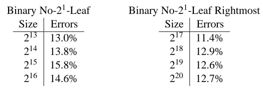
Again, there are several different methods for evaluating the performance of the learning algorithm at predicting runtimes. We begin by evaluating the performance of the learned regression tree at predicting runtimes for individual leaves. Tables 3 and 4 show this performance for a Pentium and a Sun. The errors reported are an average percentage error over all leaves in all formulas in the given test set.

Table 3: Error rates for predicting runtimes for leaves for a Pentium.

Size Errors

213 13.0%

214 13.8%

215 15.8%

216 14.6%

Size Errors

217 11.4%

218 12.9%

219 12.6%

220 12.7%

Table 4: Error rates for predicting runtimes for leaves for a Sun.

Size Errors

213 _8.7%

214 8.7%

215 10.9%

216 7.3%

Size Errors

217 _16.5%

218 16.9%

219 18.9%

220 20.0%

In all cases, the average error rate for predicting runtimes for leaves was not greater than 20%. Note that this task is considerably more difficult than predicting categories for cache misses, since the regression tree is predicting a real valued runtime instead of just one of a few categories.

(15)

split tree and summing these predictions to determine the predicted runtime for the entire formula. Again we calculate an average percentage error, but this time over entire formulas. Tables 5 and 6 show this performance.

Table 5: Error rates for predicting runtimes for entire formulas for a Pentium.

Size Errors

213 20.1%

214 22.6%

215 25.0%

216 18.1%

Size Errors

217 14.4%

218 14.1%

219 12.5%

220 10.1%

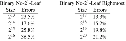
Table 6: Error rates for predicting runtimes for entire formulas for a Sun.

Size Errors

213 23.5%

214 17.6%

215 25.8%

216 36.5%

Size Errors

217 13.3%

218 15.2%

219 19.8%

220 21.2%

Unfortunately, the error rates in some cases are fairly large. Further, the error rates for predicting runtimes for entire formulas on a Pentium are considerably larger than the error rates for predicting cache misses for entire formulas. However, runtimes for formulas take on a whole range of values whereas cache misses for formulas were much more concentrated at specific values, making cache misses easier to predict.

Fortunately, we really only need a predictor that accurately orders formulas according to their runtimes. We do not need to be able to accurately predict the actual runtime of formulas, but just to predict which formula will run faster than another.

To evaluate this, we have plotted the actual runtimes of formulas against their predicted run-times. Figures 8 and 9 show these plots for two particular sizes. Each dot in the scatter plots corre-sponds to one formula in the test set with the placement corresponding to the formula’s actual and predicted runtimes. The plots show that as the predicted runtimes decrease so do the correspond-ing actual runtimes. Further, the formulas with the fastest runtimes also have the fastest predicted runtime or nearly the fastest predicted runtime.

Ideally, these plots should be simply a segment along the straight line y=x. However, the

scatter plots show that there is some spread in that formulas with the same predicted runtimes have different actual runtimes and vice versa. Further, the slope of the plots seems not to be perfectly

one. For example, in Figure 9, the W HT(214)formulas on the Sun predicted to take about 2.5×106

CPU cycles actually take about 2×106_{CPU cycles. This systematic skew may account for much}

of the error shown in Tables 5 and 6.

(16)

While the error rates at predicting runtimes were larger than we may have liked, these plots show that the learned regression trees could still be used to find fast formulas. This is surprisingly good considering that the regression trees were trained only on data from formulas of one particular size.

Binary No-21-Leaf Binary No-21-Leaf

W HT(214) Rightmost W HT(220)

1e+06 1.5e+06 2e+06 2.5e+06 3e+06 3.5e+06 4e+06 4.5e+06

1e+06 2e+06 3e+06 4e+06 5e+06

Actual Runtime (in CPU cycles)

Predicted Runtime (in CPU cycles)

1.5e+08 2e+08 2.5e+08 3e+08 3.5e+08 4e+08

Figure 8: Actual vs. predicted runtimes for entire formulas for a Pentium.

Binary No-21-Leaf Binary No-21-Leaf

W HT(214) Rightmost W HT(220)

500000 1e+06 1.5e+06 2e+06 2.5e+06 3e+06

1e+06 2e+06 3e+06 4e+06

5e+07 1e+08 1.5e+08 2e+08 2.5e+08 3e+08

5e+07 1e+08 1.5e+08 2e+08

Figure 9: Actual vs. predicted runtimes for entire formulas for a Sun.

3.5 Predicting FFT Runtimes

These good results for the WHT raise the possibility of extending these techniques to other trans-forms. We chose to consider the FFT next because it is one of the most important and widely used transforms and also because it is similar to the WHT. The previous results for the WHT used a pack-age for timing different WHT formulas. The SPIRAL system provides the ability to implement in code, run, and time a wide variety of different transforms including the FFT; thus, it was the obvious choice to replace the WHT package.

(17)

is performed for each internal FFT node (this arises from the twiddle factors, T_srs, in the Cooley-Tukey factorization). Thus, the total runtime of an FFT formula is more than just the sum of the runtimes spent computing each of the leaves. So, we decided to follow a similar approach as before but now model runtime performance of not only leaves but also internal nodes.

To predict runtimes for FFTs, we decided to train up two separate predictors: one for leaves and one for internal nodes. Thus, a runtime prediction for an entire FFT split tree can be made by summing the predictions made for all of its nodes, both leaves and internal nodes, using the appropriate predictor for each node.

A runtime predictor for FFT leaves was trained exactly as was done in Section 3.4.1 for WHT leaves using the same feature set. The same method can also be used to train a predictor for FFT internal nodes as well. However, we have also explored using some additional features for internal nodes that are not applicable for leaves.

Specifically, the sizes and strides of the immediate children of an internal node add four ad-ditional features. One might expect that the way an internal node is split may affect the runtime performance of the work associated with that internal node. Further, the sizes and strides of the four grandchildren could be used as additional features, further defining the internal node’s subtree. If any of the children are leaves, then the features corresponding to the missing grandchildren are set

to−1 to indicate that the nodes do not exist. We present results using the following three different

feature sets:

• Original. The original six features as described in Section 3.2.1.

• Children. The original six features plus features describing the immediate children of the

internal node.

• Grandchildren. The original six features plus features describing the immediate children

and grandchildren of the internal node.

Again we used RT4.0 to train regression trees on data collected on the same Pentium used in the previous experiments. For the leaf predictor, we used a random 10% of the leaves from all of the

formulas generated for DFT(216). Likewise we trained regression trees using each of the different

feature sets on a random 10% of the internal nodes from all of the formulas generated for DFT(216).

3.5.2 EVALUATION

We used two different methods to evaluate these predictors for the FFT. First, we considered the average error rate for predicting runtimes for entire formulas. Second, we plotted the predicted runtime against the actual runtime for individual formulas. To do the evaluations, we generated all

possible formulas for sizes 212 to 218 and timed them. We were not confident that rightmost trees

were optimal, and so without that additional limitation it was impossible to exhaustively search up

to size 220. Results are shown using all three different feature sets to describe internal nodes, but

in all cases the original feature set was used to describe the leaves (as leaves clearly do not have children or grandchildren).

(18)

For many of the larger sizes, the error rates are less than 10%, and for no size are they greater than 20%. Further, increasing the number of features used through the children and grandchildren feature sets tends to improve the overall performance of the predictor while slightly decreasing the performance for a few of the smaller sizes.

Table 7: Error rates for predicting FFT formula runtimes on a Pentium using different feature sets.

Original Children Grandchildren

Size Errors

212 9.8%

213 15.5%

214 11.8%

215 8.7%

216 _6.4%

217 8.2%

218 8.9%

Size Errors

212 11.8%

213 15.2%

214 9.6%

215 7.6%

216 _5.6%

217 7.8%

218 8.8%

Size Errors

212 19.3%

213 9.3%

214 10.7%

215 7.3%

216 _5.0%

217 7.3%

218 7.9%

Figure 10 shows scatter plots of the actual versus predicted runtimes for FFT formulas on the same Pentium machine. The plots show predictions for formulas of two different sizes and using the three different feature sets. Each point in the plots corresponds to one formula with the point placed according to the formula’s actual and predicted runtimes. Ideally all the points would fall

along the line y=x indicating that the predicted runtime equaled the actual runtime.

While there is some spread, most of the points fall very close to the ideal line y=x. Further,

the formulas with the fastest predicted runtimes are those formulas with the fastest actual runtimes. Visually, the major difference between the different feature sets is that increasing the number of features seems to improve the overall slope so that the predicted runtimes of the fastest formulas are more accurate.

The learned regression trees perform well at ordering formulas according to their runtimes, predicting faster formulas to have smaller runtimes. Once again, these are particularly excellent results considering that the learned regression trees were only trained on data from transforms of

size 216and here are predicting for both smaller and larger sizes.

3.6 Summary

We have presented a method for predicting a WHT formula’s number of cache misses on a Pentium by training a decision tree to predict a leaf’s number of cache misses to be one of only a few categories. We have also shown that this method produces very good results across sizes even when only trained on one particular size.

We have presented a similar method for predicting runtimes instead of cache misses for WHT formulas. This method can be used on any machine and we demonstrated its performance on two very different architectures. The learned regression trees are able to perform very well at ordering formulas according to their runtimes, especially considering that the regression trees were trained on data of one size and used to predict across many transform sizes including larger sizes.

(19)

214 218

O

riginal

4e+06 6e+06 8e+06 1e+07 1.2e+07 1.4e+07 1.6e+07

4e+06 6e+06 8e+06 1e+07 1.2e+071.4e+071.6e+07

1e+08 2e+08 3e+08 4e+08 5e+08

C

h

ildren

4e+06 6e+06 8e+06 1e+07 1.2e+07 1.4e+07 1.6e+07

4e+06 6e+06 8e+06 1e+07 1.2e+071.4e+071.6e+07

1e+08 2e+08 3e+08 4e+08 5e+08

G

randchildren

4e+06 6e+06 8e+06 1e+07 1.2e+07 1.4e+07 1.6e+07

4e+06 6e+06 8e+06 1e+07 1.2e+071.4e+071.6e+07

1e+08 2e+08 3e+08 4e+08 5e+08

(20)

obtained excellent results, with the regression trees accurately predicting runtimes for FFT formulas. While the predictors were only trained on data from one transform size, they accurately predicted for both smaller and larger transform sizes.

4. Generating Optimal Implementations

Accurate prediction of runtimes still does not solve the problem of determining the fastest formula from a very large number of candidates. At larger sizes, it is infeasible to just enumerate all possible formulas, let alone obtain predicted runtimes for all of them in order to choose the fastest. While our work in predicting performance for formulas allowed for runtimes to be predicted much more quickly than the formulas could be timed, it still did not provide a method that quickly produced formulas with fast runtimes.

In this section, we present a method that learns to generate formulas with fast runtimes. Out of the very large space of possible formulas, our method learns how to control the generation of formulas to produce the formulas with the fastest runtimes. Remarkably, our new method can be trained on data from a particular sized transform and still construct fast formulas across many sizes. Thus, our method can generate fast formulas for many sizes, even when not a single formula of those sizes has been timed yet.

The learned decision and regression trees that predict performance of WHT and FFT nodes are used here as the sole source of runtime information for a given platform. By using a number of concepts from reinforcement learning combined with these predictors, our method is able to generate formulas that have the fastest known runtimes.

We begin by describing our initial approach to the problem and how it led to the algorithm we have designed and implemented. After discussing this algorithm, we then provide other views of our method. Finally, we evaluate our method’s performance for two different machines and two different transforms.

4.1 Approach

We approach the question of generating fast formulas as a control learning problem. We first try to formulate the problem in terms of a Markov decision process (MDP) and reinforcement learning. In the end, our formulation is not an MDP but does borrow many concepts from reinforcement learning.

4.1.1 BASICFORMULATION

An MDP is a tuple (

S

,

A

,T,C), where

S

is a set of states,

A

is a set of actions, T :

S

×

A

→

S

is a transition function that maps the current state and action to the next state, and C:

S

×

A

→ℜ

is a cost function that maps the current state and action onto its real valued cost. Reinforcement

learning provides methods for finding a policy π:

S

→

A

that selects the best action at each state

that minimizes the (possibly discounted) sum of costs incurred.

(21)

20 ₂₀

4 16

20

4 16

2 2

(a) (b) (c)

Figure 11: Example of growing a fast WHT split tree.

We now turn to trying to formulate this problem in terms of MDPs. Let the states in the re-inforcement learning problem be nodes in a split tree that have no children but have not yet been decided to be leaves. Then the start state is just a root node of the given transform and size with no children. The actions in each state are the different ways to grow children for that node or to leave the node as a leaf (if the node’s size is small enough).

Ideally, the cost function should be as follows:

• the leaf’s runtime (or cache misses) when making a node a leaf, and

• the internal node’s runtime when giving children to a node.

Note that for the WHT, there is no runtime associated with internal nodes, and thus the cost function would be zero when giving children to a node. The total cost of growing an entire split tree is then the runtime of the entire formula. The goal is to minimize the sum of the undiscounted costs over building an entire split tree.

4.1.2 DETAILS ANDDIFFICULTIES

There are a number of details that need to be filled in with respect to this basic formulation. Further, one significant difficulty also becomes apparent upon trying to fill in these details.

State Representation We need a state representation for the nodes within a split tree so that we can use standard reinforcement learning algorithms. For the WHT, we have used the leaf features described in Section 3.2.1 that expands the feature set to describe any node in a split tree. For the FFT, we have used the same features, but also the two additional feature sets used to describe internal nodes that were introduced in Section 3.5.1.

Cost Function Ideally, we would use the actual runtime of leaves and internal nodes to determine the cost function. However, this requires determining the runtime for these nodes even when the split tree is not fully grown. Unfortunately, it is not possible to run a partially grown split tree with the SPIRAL system or with the WHT package we are using.

However, we have already discussed how we can easily learn to predict cache misses or runtimes for leaves and internal nodes. So, we can approximate our desired cost function by using these learned predictors. In particular, we will use the following cost function:

• the leaf’s predicted performance when making a node a leaf,

(22)

• the internal node’s predicted performance when giving children to a FFT node. The predictors have several advantages:

• They can make predictions much quicker than we could time a formula (even if we had a

formula to time in this case).

• Since they are using the same features to describe nodes as we are using to describe nodes in

our MDP state space, no extra work needs to be done to translate features.

This change causes our method to rely on the predictors and to only be as good as they are. Further, if a cache miss predictor is used, then our method will construct formulas with minimal cache misses, instead of explicitly constructing the fastest formulas. However, on a Pentium we have shown that the fastest WHT formulas have the minimal number of cache misses.

Also the choice of predictor can influence how many formulas are generated with the same expected performance. Since there are many formulas with the same number of cache misses and our cache miss predictor produces discrete valued outputs, it would be expected that using a cache miss predictor will cause our algorithm to generate several formulas with the same expected perfor-mance. On the other hand, runtimes tend to be much more continuous, and so it is likely that using a runtime predictor will lead to many fewer formulas with the exact same predicted performance.

Transition Function Defining a transition function for this formulation is difficult. If two children of the root node are grown, then several questions arise, such as: which node is the next state, when will we transition back to the sibling node, and what should the transition function be from a leaf node? It is possible to answer these questions in specific ways, but then the Markov property may no longer hold. Lagoudakis and Littman (2000) discuss one approach for coping with this difficulty. They determine the Monte Carlo return for all but one of the next states, fixing the current policy. Then they continue learning on the one remaining next state. However, we can take a different approach, departing from the MDP framework, since we can formulate our problem to be deterministic and off-line.

Actions are deterministic in that a node will always be given the children, if any, specified by the action. The cost function is deterministic and known if we use a learned predictor. We will define a value function over our states and show how it can be computed off-line.

4.1.3 VALUEFUNCTION

First consider a value function over nodes in a fully specified split tree. The value of an internal node is the sum of the performance measures of all the nodes in the subtree rooted at the internal node. More formally,

V(node) =

∑

leaf∈subtree

PredictedPerformance(leaf)

+

∑

internalNode∈subtree

PredictedPerformance(internalNode)

where the PredictedPerformance of an internal WHT node is zero. Thus, the value of the root node is the performance of the entire split tree. We can rewrite this value function recursively in terms of the values of the children of the given node:

V(node) =

PredictedPerformance(node),if node is a leaf

(23)

Now we will define the optimal value function over the specified state space. If a state must be a leaf, then its value is its predicted performance. However, the optimal value of a node that could be an internal node or a leaf must consider both possibilities. If a state can have children, then we wish to find the subtree (possibly the subtree that simply makes the node a leaf) that minimizes the predicted performance summed over all the nodes. That is,

V∗(state) =minsubtrees

∑

leaf∈subtree

PredictedPerformance(leaf)

+

∑

internalNode∈subtree

PredictedPerformance(internalNode).

Again, we can rewrite this value function recursively in terms of the values of the possible children of the state. The optimal value of a state is the sum of the values of all the children in the optimal subtree rooted at this state, or the predicted performance if the optimal subtree for the state is to be a leaf. Mathematically, let the leaf performance of a state be:

LeafPerf(state) =

PredictedPerformance(state),if state can be a leaf

∞,if state cannot be a leaf

and the splitting value of a node be:

SplitV(state) = min

splittingsPredictedPerformance(state) +_child_∈

∑

_splittingV

∗₍_child₎_,

where the minimum over splittings minimizes over all possible sets of immediate children of a state and has a value of infinity if the state cannot have children. Then,

V∗(state) =min{LeafPerf(state),SplitV(state)}.

If the children or grandchildren feature sets are used, then the state space already captures the immediate children. In these cases, SplitV ’s minimum must be taken over all possible grandchildren or great-grandchildren. While the child is determined from the state of the given node, the child’s full state feature values must account for the chosen grandchildren or great-grandchildren.

4.2 Algorithm

This recursive formulation of the value function suggests dynamic programming for computing it. For any state that could be a leaf, we can determine its value as a leaf by querying the predictor to get its predicted performance. For any state that could have children, the dynamic programming routine can then recursively call itself with each of the possible children, memoizing computed values for

efficiency. The algorithm is shown in Table 8. For the WHT, let thePredictedPerformance of

internal nodes be zero.

(24)

Table 8: Algorithm for computing values of states. ComputeValues(State)

if V(State) already memoized return V(State)

Min = ∞

if State can be a leaf

Min = PredictedPerformance(State)

for SetOfChildren in PossibleSetsOfChildren(State) Sum = 0

for Child in SetOfChildren Sum += ComputeValues(Child) Sum += PredictedPerformance(State)

if Sum < Min

Min = Sum V(State) = Min return Min

While ComputeValues considers all possible sets of children of a given state, it is considerably more efficient than exhaustively constructing all possible split trees and making performance pre-dictions for them. By computing and memoizing values of states, ComputeValues saves significant

computation over an exhaustive search approach. For example, suppose we split W HT(220₎ _into

W HT(28) and W HT(212). Then if we were performing exhaustive search, we would have to

re-compute the value for all possible subtrees of W HT(28)every time we choose a different possible

subtree for W HT(212₎_{(and there are many possible trees for both). Since ComputeValues}

memo-izes its results, it only has to compute a value once for W HT(28)as the left child of the root and

once for W HT(212)as the right child of the root.

Note that ComputeValues cannot easily keep track of the best split tree as there may be several formulas with the best predicted performance. This is particularly true when using a cache miss predictor since many formulas have exactly the same number of cache misses.

With the value function determined for all relevant states, the next step is to produce fast formu-las. For a given size, the algorithm looks up the value of a root node of that size. It then considers all possible sets of children of the root node and determines their values. Any set of children whose sum of values equals the root node’s value is then predicted to be one of the fastest way to split the root node. This procedure is then repeated for each child, building up a set of fast split trees.

The algorithm for generating fast split trees is shown in Table 9. Leaf() creates a leaf node from the given state, Node() creates a split tree node with the corresponding subtrees as children, and MatchingChild() creates the state for the left child of the specified state when given the right child. As before, the loop over possible children would need to be modified to loop over possible grandchildren or great-grandchildren if the FFT feature sets children or grandchildren are used.

(25)

Table 9: Algorithm for generating fast split trees. FastTrees(State)

Trees = {}

if State can be a leaf

if V(State) == PredictedPerformance(State)

Trees = { Leaf(State) }

for RightChild in PossibleRightChildren(State) LeftChild = MatchingChild(State, RightChild) if V(LeftChild) + V(RightChild)

+ PredictedPerformance(State) == V(State) for RightSubtree in FastTrees(RightChild)

for LeftSubtree in FastTrees(LeftChild)

Trees = Trees ∪ { Node(LeftSubtree, RightSubtree) }

return Trees

allow for a tolerance. This algorithm produces split trees with runtimes or cache misses within the specified tolerance of the optimal predicted performance.

4.3 Other Views

Section 4.1 presented our original approach to the problem. However, the final algorithm can be viewed in other ways.

The algorithm we have presented is similar to solving an MDP. However, we did not give a well defined transition function for this problem, and thus did not actually frame it as an MDP. We do have a model of the system in that we know what actions do and we know the cost function since it is represented by the learned predictor. This allows us to compute the value function off-line.

Since a node’s value only depends on the possible subtrees that could be grown underneath it, dynamic programming is an efficient method for computing the value function. Dynamic program-ming has been frequently used to find fast implementations of signal transforms (Johnson and Bur-rus, 1983; Frigo and Johnson, 1998; Haentjens, 2000; Sepiashvili, 2000); however, our approach is significantly different from these previous approaches. We use the learned regression trees to evaluate different choices while the previous approaches actually implemented and timed differ-ent choices. Further, we use a rich feature set to distinguish between nodes, while the previous approaches only found one good implementation for each size.

Thus, this problem is well suited for using dynamic programming. The problem has overlapping subproblems in that the value for a particular state is repeatedly needed as illustrated in the above example. Further, by using a powerful state space representation that captured information about the location of a node in a split tree, we could assume optimal substructure — that is, optimal solutions to the problem contain optimal solutions to subproblems. Consider again the example

of splitting W HT(220)into W HT(28)and W HT(212). The best subtree for the W HT(28)node is

largely independent of the subtree grown for the W HT(212₎_{node, but it is dependent on the fact}

that the W HT(28)node was the left child of the W HT(220)root node. The features chosen capture

(26)

4.4 Evaluation

Evaluating our method is difficult since the optimal formula for larger sizes is unknown. However, for the WHT, we can compare our algorithm against the best formulas found by searches over

limited portions of the space as we did to evaluate the predictors. That is, for sizes 216and smaller

we exhaustively search over all binary WHT formulas with no leaves of size 21, and for sizes 217

and larger we exhaustively search over all rightmost binary WHT formulas with no leaves of size

21. These subspaces of WHT formulas contain the fastest formulas found from performing a variety

of different searches. For the FFT, we exhaustively search over the defined space and compare our

results, but this is only possible up to about size 218(which took a considerable amount of time to

collect the data).

We have used the decision tree learned in Section 3.2 that predicted cache misses for WHT leaves and the regression trees learned in Section 3.4 that predicted runtimes for WHT leaves. Fur-ther, we used the regression trees learned in Section 3.5 that predicted runtimes for FFT nodes. Since these decision and regression trees were trained on leaves from binary trees with no leaves

of size 21, our algorithm only constructs binary trees with no leaves of size 21. This can be easily

extended by training a decision or regression tree on a broader class of formulas.

4.4.1 USING THEWHT CACHEMISS PREDICTOR

We begin with results from using the learned decision tree that predicted cache misses for WHT leaves on a Pentium. Since many split trees can have the same number of cache misses, it is not surprising that many states have the same value, and thus our algorithm produces several trees that it predicts to be fast. Table 10 displays three different results for different sizes.

Table 10: Results from generating fast WHT formulas using a Pentium cache miss predictor.

Number of Generated Top N Fastest

Formulas Included the Known Formulas

Size Generated Fastest Known in Generated

212 101 yes 77

213 86 yes 4

214 101 yes 70

215 86 yes 11

216 101 yes 68

217 86 yes 15

218 ₁₀₁ _yes ₂₅

219 86 yes 16

220 101 yes 16

(27)

learning algorithm generates the fastest known formulas for all sizes, including sizes larger than the training size.

The last column shows the largest n where all n of the fastest formulas found by a limited

exhaustive search were also generated by our method. For example, for size 220, our method

con-structed all of the fastest 16 formulas found by a limited exhaustive search, but did not generate the 17th fastest formula. For all sizes, our method generates the fastest formula as well as many of the formulas that are very close to the fastest.

Figure 12 compares the histograms of runtimes for W HT(220)formulas generated by our method

and for all rightmost binary W HT(220) formulas with no leaves of size 21. Notice the different

scales along both axes. Clearly our method is constructing formulas with runtimes amongst the fastest found by the more exhaustive method.

1.5 2 2.5 3 3.5 4

x 108 0

20 40 60 80 100 120 140 160 180

Running Time in CPU Cycles

Number of Formulas

1.6 1.8 2 2.2 2.4

x 108 0

1 2 3 4 5 6

Running Time in CPU Cycles

Number of Formulas

(a) (b)

Figure 12: Histograms of runtimes for (a) all rightmost binary W HT(220)formulas with no leaves

of size 21 and (b) the formulas generated by our method for W HT(220)using a cache

miss predictor on Pentium data.

4.4.2 USINGWHT RUNTIMEPREDICTORS

Next, we use the learned regression trees that predicted runtimes for WHT leaves with our method. Here we evaluate the approach both on Pentium and Sun data. We have used the same learned regression trees as were described and evaluated in Section 3.4 and that were trained using data

from 500 random W HT(216)split trees with no leaves of size 21.

Because the learned regression trees predict real-valued runtimes instead of only one of a few categories, most formulas have different predicted runtimes. So, our generation method normally would only produce a single formula which it believes to run as fast as possible. To evaluate, we have given our generation method a tolerance and had it generate all formulas that it believes will have up to that tolerance more runtime than the predicted fastest one. We began with a small tolerance and increased it as necessary to generate as many formulas as necessary to perform the evaluations described below.

(28)

shows when during the generation process the best known formula (through a limited exhaustive

search) is generated. For example, on the Pentium (Table 11) the fourth W HT(220)formula

gen-erated by our method is the fastest known formula, while the first three formulas gengen-erated by our method were actually slower than this fourth one.

Table 11: Evaluation of generation method using a WHT runtime predictor for a Pentium.

Size

Generated formula X is

best known

formula

First generated for-mula is X % slower than best known formula

Number of top 100 best known formulas in top 100 generated formulas

First best known for-mula not in top 100 generated formulas

213 5 3.4% 69 19

214 4 3.0% 63 19

215 3 2.1% 68 16

216 4 1.7% 63 18

217 5 0.1% 54 36

218 4 2.0% 60 24

219 1 0.0% 44 36

220 4 1.7% 64 24

Table 12: Evaluation of generation method using a WHT runtime predictor for a Sun.

Size

Generated formula X is

best known

formula

First generated for-mula is X % slower than best known formula

Number of top 100 best known formulas in top 100 generated formulas

First best known for-mula not in top 100 generated formulas

213 14 77.7% 20 6

214 20 12.8% 70 24

215 ₁ _0.0% ₆₈ ₃₈

216 2 4.3% 70 20

217 7 18.0% 47 10

218 38 5.9% 46 7

219 17 3.3% 46 4

220 47 1.4% 52 4

The third column shows how much slower the first generated formula is compared to the fastest known formula. The fourth column shows how many of top 100 fastest known formulas are gener-ated if we allow our method to only generate 100 formulas. Finally the fifth column shows the first best known formula that was not in the top 100 formulas generated.

These results are excellent, especially considering the fact that our method only uses training

data from one size (216in this case). Our method always generated the fastest known formula within

(29)

had a runtime within 6% or less of the fastest known formula. Again this is great considering that the formulas of the same size can have a factor of 2–10 spread in runtimes.

Also, our method was able to generate about 50 of the top 100 fastest known formulas even when our method was limited to generating only 100 formulas. For the Pentium, our method was also able generate all of the top 15 formulas for each size (often many more) while being limited to generating only 100 formulas. For the Sun, our method was sometimes unable to generate the fourth fastest known formula for a few particular sizes when being limited to generating only 100 formulas.

Overall, our method more easily generates fast formulas for the Pentium than for the Sun, but still for the Sun our method is able to generate the fastest known formula in the first 50 formulas that it produces. Thus, by timing a few random formulas of one particular size to be used as training data, our method can be used to generate very fast formulas for different transform sizes including larger sizes. Often the very first formula it produces has a runtime very close to the fastest known formula. Further, if one is willing to time a few additional formulas for each size, the fastest known formula can be found. While we have evaluated our method on a Pentium and a Sun, our method should work across any architecture. Our method does not depend on any observations specific to those machines.

4.4.3 USINGFFT RUNTIMEPREDICTORS

Finally, we used the learned regression trees that predicted runtimes for FFT nodes. We evaluate these predictors in a similar manner as the WHT runtime predictors, but this time we evaluate across the three different feature sets. We evaluate against an exhaustive search of all possible formulas

from the space we considered (see Section 2.4) for sizes 212_{to 2}18_{. Recall that the trained regression}

trees were trained only on data for FFTs of size 216.

Table 13 displays the results of using our generation method to construct fast FFT implementa-tions. With any of the feature sets, our method was able to construct the fastest known FFT formula

of sizes 214to 216within the first 10 formulas that it generated. However, the grandchildren feature

set tends to outperform the other feature sets. Using the grandchildren feature set, our method was able to generate the fastest known formula as its first produced formula for three of the sizes. Fur-ther, for the other sizes, either the first generated formula was nearly as fast as the best known or the best known formula was generated within the first several formulas generated.

Again these results are excellent considering the huge search space of formulas and the wide

spread of runtimes. Further, our method has only seen timings for formulas of size 216and yet can

construct fast formulas for both smaller and larger sizes.