Distributed Algorithms for Topic Models

Distributed Algorithms for Topic Models

David Newman [email protected]

Arthur Asuncion [email protected]

Padhraic Smyth [email protected]

Max Welling [email protected]

Department of Computer Science University of California, Irvine Irvine, CA 92697, USA

Editor: Andrew McCallum

Abstract

We describe distributed algorithms for two widely-used topic models, namely the Latent Dirichlet Allocation (LDA) model, and the Hierarchical Dirichet Process (HDP) model. In our distributed algorithms the data is partitioned across separate processors and inference is done in a parallel, distributed fashion. We propose two distributed algorithms for LDA. The first algorithm is a straightforward mapping of LDA to a distributed processor setting. In this algorithm processors concurrently perform Gibbs sampling over local data followed by a global update of topic counts. The algorithm is simple to implement and can be viewed as an approximation to Gibbs-sampled LDA. The second version is a model that uses a hierarchical Bayesian extension of LDA to di-rectly account for distributed data. This model has a theoretical guarantee of convergence but is more complex to implement than the first algorithm. Our distributed algorithm for HDP takes the straightforward mapping approach, and merges newly-created topics either by matching or by topic-id. Using five real-world text corpora we show that distributed learning works well in prac-tice. For both LDA and HDP, we show that the converged test-data log probability for distributed learning is indistinguishable from that obtained with single-processor learning. Our extensive ex-perimental results include learning topic models for two multi-million document collections using a 1024-processor parallel computer.

Keywords: topic models, latent Dirichlet allocation, hierarchical Dirichlet processes, distributed

parallel computation

1. Introduction

Very large data sets, such as collections of images or text documents, are becoming increasingly common, with examples ranging from collections of online books at Google and Amazon, to the large collection of images at Flickr. These data sets present major opportunities for machine learn-ing, such as the ability to explore richer and more expressive models than previously possible, and provide new and interesting domains for the application of learning algorithms.

on a typical desktop computer. If one were to assume that a simple operation, such as computing a probability vector over categories using Bayes rule, takes on the order of 10−6seconds per word, then a full pass through the billion words would take 1000 seconds. Thus, algorithms that make multiple passes through the data, for example clustering and classification algorithms, will have run times in days for this sized corpus. Furthermore, for small to moderate sized document sets where memory is not an issue, it would be useful to have algorithms that could take advantage of desktop multiprocessor/multicore technology to learn models in near real-time.

An obvious approach for addressing these time and memory issues is to distribute the learning algorithm over multiple processors. In particular, with P processors, it is somewhat trivial to address the memory issue by distributing _P1 of the total data to each processor. However, the computation problem remains non-trivial for a fairly large class of learning algorithms, namely how to combine local processing on each processor to arrive at a useful global solution.

In this general context we investigate distributed algorithms for two widely-used unsupervised learning models: the Latent Dirichlet Allocation (LDA) model, and the Hierarchical Dirichet Pro-cess (HDP) model. LDA and HDP models are arguably among the most sucPro-cessful recent learning algorithms for analyzing discrete data such as bags of words from a collection of text documents. However, they can take days to learn for large corpora, and thus, distributed learning would be particularly useful.

The rest of the paper is organized as follows: In Section 2 we review the standard derivation of LDA and HDP. Section 3 presents our two distributed algorithms for LDA and one distributed algorithm for HDP. Empirical results are provided in Section 4. Scalability results are presented in Section 5, and further analysis of distributed LDA is provided in Section 6. A comparison with related models is given in Section 7. Finally, Section 8 concludes the paper.

2. Latent Dirichlet Allocation and Hierarchical Dirichlet Process Model

We start by reviewing the LDA and HDP models. Both LDA and HDP are generative probabilistic models for discrete data such as bags of words from text documents—in this context these models are often referred to as topic models. To illustrate the notation, we refer the reader to the graphical models for LDA and HDP shown in Figure 1.

LDA models each of D documents in a collection as a mixture over K latent topics, with each topic being a multinomial distribution over a vocabulary of W words. For document j, we first draw a mixing proportionθj from a Dirichlet with parameterα. For the ithword in the document,

a topic zi j=k is drawn with probabilityθk|j. Word xi j is then drawn from topic zi j, with xi j taking

on value w with probabilityφw|zi j. A Dirichlet prior with parameterβis placed on the word-topic distributionsφk.

Thus, the generative process for LDA is given by

θj∼

D

D

D

D

un-less specified otherwise. The full joint distribution over all parameters and variables is

p(x,z,θ,φ|α,β) =

∏

Γ(Kα) Γ(α)K ∏kθ

Nk j+α−1

k|j

∏

Γ(Wβ) Γ(β)W ∏wφ

Nwk+β−1

α

ij

Z

ij

X k

φ

j

θ

k

α

ij

Z

ij

X

j

θ

k

φ

K D

N_j

∞

β

β

γ

η

Figure 1: Graphical models for LDA (left) and HDP (right). Observed variables (words) are shaded, and hyperparameters are shown in squares.

Description

D Number of documents in collection

W Number of distinct words in vocabulary

N Total number of words in collection

K Number of topics

xi j ithobserved word in document j zi j Topic assigned to xi j

Nwk Count of word assigned to topic Nk j Count of topic assigned in document φk Probability of word given topic k θj Probability of topic given document j

Table 1: Description of commonly used variables.

where Nwk j=#{i : xi j =w,zi j =k}, and we use the convention that missing indices are summed

out. Nk j=∑wNwk j and Nwk =∑jNwk j are the two primary count arrays used in computations,

representing the number of words assigned to topic k in document j, and the number of times word

w is assigned to topic k in the corpus, respectively. For ease of reading we list commonly used

variables in Table 1.

Given the observed words x={xi j}, the task of Bayesian inference for LDA is to compute the posterior distribution over the latent topic assignments z={zi j}, the mixing proportionsθj, and the

topicsφk. Approximate inference for LDA can be performed either using variational methods (Blei

the conditional probability of zi jis

p(zi j=k|z¬i j,x,α,β)∝

N_wk¬i j+β ∑wN

¬i j wk +Wβ

N_{k j}¬i j+α, (3)

where the superscript¬i j means that the corresponding word is excluded in the counts.

HDP is a collection of Dirichlet Processes which share the same topic distributions and can be viewed as the non-parametric extension of LDA. The advantage of HDP is that the number of topics is determined by the data. The HDP model is obtained by taking the following model in the limit as

K goes to infinity. Letαk be top level Dirichlet variables sampled from a Dirichlet with parameter γ/K. The topic mixture for each document, θj, is drawn from a Dirichlet with parameters ηαk.

The word-topic distributionsφk are drawn from a base Dirichlet distribution with parameterβ. As

in LDA, zi j is sampled from θj, and word xi j is sampled from the corresponding topic φzi j. The generative process is given by

αk∼

D

The posterior distribution is sampled using the direct assignment sampler for HDP described in Teh et al. (2006). As was done for LDA, bothθandφare integrated out, and zi j is sampled from

the following conditional distribution:

p(zi j=k|z¬i j,x,α,β,η)∝



 

 

N_wk¬i j+β

∑wNwk¬i j+Wβ

N_{k j}¬i j+ηαk

, if k previously used

ηαnew

W , if k is new.

(4)

The sampling scheme forαk is also detailed in Teh et al. (2006). Note that a small amount of

probability mass proportional toαnewis reserved for the instantiation of new topics. While HDP is

defined to have infinitely many topics, the sampling algorithm only instantiates topics as needed.

2.1 Need for Distributed Algorithms

One could argue that it is trivial to distribute non-collapsed Gibbs sampling, because sampling of zi j can happen independently givenθj andφk, and therefore can be done concurrently. In the

non-collapsed Gibbs sampler, one samples zi jgivenθjandφk, and then samplesθjandφkgiven zi j.

Furthermore, if individual documents are not spread across different processors, one can marginalize over justθj, sinceθjis processor-specific. In this partially collapsed scheme, the latent variables zi j

on each processor can be concurrently sampled, where the concurrency is over processors.

Unfortunately, the non-collapsed and partially collapsed Gibbs samplers exhibit slow conver-gence due to the strong dependencies between the parameters and latent variables. Generally, we expect faster mixing as more variables are collapsed (Liu et al., 1994; Casella and Robert, 1996). Figure 2 shows, using one of the data sets used throughout our paper, that the log probability of test data (measured as perplexity, which is defined in Section 4) of the non-collapsed and partially collapsed samplers converges more slowly than the fully collapsed sampler.

0 200 400 600 800 1000 1800

1850 1900 1950 2000 2050 2100 2150 2200

Iteration

Perplexity

Non−Collapsed

θ Collapsed

θ, φ Collapsed

Figure 2: On the NIPS data set using K=20 topics, the fully collapsed Gibbs sampler (solid line) converges faster than the partially collapsed (circles) and non-collapsed (triangles) sam-plers.

3. Distributed Algorithms for Topic Models

We introduce algorithms for LDA and HDP where the data, parameters, and computation are dis-tributed over distinct processors. We distribute the D documents over P processors, with approx-imately DP = D_P documents on each processor. Documents are randomly assigned to processors,

although as we will see later, the assignment of documents to processors—ranging from random to highly non-random or adversarial—appears to have little influence on the results. This indifference is somewhat understandable given that converged results from Gibbs sampling are independent of sampling order.

We partition the words from the D documents into x={x1, . . . ,xp, . . . ,xP}and the

correspond-ing topic assignments into z={z1, . . . ,zp, . . . ,zP}, where processor p stores xp, the words from

doc-uments j= (p−1)DP+1, . . . ,pDP, and zp, the corresponding topic assignments. Topic-document

counts Nk j are likewise distributed as Nk j p. The word-topic counts Nwk are also distributed, with

each processor keeping a separate local copy Nwk p.

3.1 Approximate Distributed Latent Dirichlet Allocation

The difficulty of distributing and parallelizing over Gibbs sampling updates (3) lies in the fact that Gibbs sampling is a strictly sequential process. To asymptotically sample from the posterior distri-bution, the update of any topic assignment zi j can not be performed concurrently with the update

of any other topic assignment zi′_j′. But given the typically large number of word tokens compared to the number of processors, to what extent will the update of one topic assignment zi j depend on

Algorithm 1 AD-LDA repeat

for each processor p in parallel do

Copy global counts: Nwk p←Nwk

Sample zplocally: LDA-Gibbs-Iteration(xp, zp, Nk j p, Nwk p,α,β) end for

Synchronize

Update global counts: Nwk←Nwk+∑p(Nwk p−Nwk) until termination criterion satisfied

(i.e., wi j 6=wi′_j′), then concurrent sampling will be very close to sequential sampling because the only term affecting the order of operations is the total count of topics∑wNwk in the denominator of

(3).

The pseudocode for our Approximate Distributed LDA (AD-LDA) algorithm is shown in Algo-rithm 1. After distributing the data and parameters across processors, AD-LDA performs simultane-ous LDA Gibbs sampling on each of the P processors. After processor p has swept through its local data and updated topic assignments zp, the processor has modified count arrays Nk j pand Nwk p. The

topic-document counts Nk j p are distinct because of the document index, j, and will be consistent

with the topic assignments z. However, the word-topic counts Nwk p will in general be different on

each processor, and not globally consistent with z. To merge back to a single and consistent set of word-topic counts, we perform a reduce operation on Nwk p across all processors to update the

global counts. After the synchronization and update operations, each processor has the same val-ues in the Nwk parray which are consistent with the global vector of topic assignments z. Note that Nwk pis not the result of P separate LDA models running on separate data. In particular, each

word-topic count array reflects all the counts, not just those local to that processor, so for every processor

∑wkNwk p=N, where N is the total number of words in the corpus. As in LDA, the algorithm can

terminate either after a fixed number of iterations, or based on some suitable MCMC convergence metric.

We chose the name Approximate Distributed LDA because in this algorithm we are no longer asymptotically sampling from the true posterior, but to an approximation of the true posterior. Nonetheless, we will show in our experimental results that the approximation made by Approxi-mate Distributed LDA works very well.

3.2 Hierarchical Distributed Latent Dirichlet Allocation

In AD-LDA we constructed an algorithm where each processor is independently computing an LDA model, but at the end of each sweep through a processor’s data, a consistent global array of topic counts Nwkis reconstructed. This global array of topic counts could be thought of as a parent topic

distribution, from which each processor draws its own local topic distribution.

Using this intuition, we created a Bayesian model reflecting this structure, as shown in Fig-ure 3. Our Hierarchical Distributed LDA model (HD-LDA) places a hierarchy over word-topic distributions, withΦk being the global or parent word-topic distribution and ϕk p the local

word-topic distributions on each processor. The local word-word-topic distributionsϕk p are drawn fromΦk

according to a Dirichlet distribution with a topic-dependent strength parameter βk, for each topic

jp

θ

γ

a b

,

c d

k

β

p

α

ijp

Z

ijp

X

k

Φ

kp

ϕ

K

P Nj p

D_p

P

Figure 3: Graphical model for Hierarchical Distributed Latent Dirichlet Allocation.

by:

βk∼

G

G

D

D

D

From this generative process, we derive Gibbs sampling equations for HD-LDA. The derivation is based on the Teh et al. (2006) sampling schemes for Hierarchical Dirichlet Processes. As was done for LDA, we start by integrating out ϕ andθ. The collapsed distribution of zp and xp on

processor p is given by:

p(zp,xp|αp,β,Φ) =

∏

"

Γ(Kαp) Γ(Nj p+Kαp)

∏

Γ(Nk j p+αp) Γ(αp)

#

∏

Γ

(βk) Γ(Nk p+βk)

∏

Γ(Nwk p+βkΦw|k) Γ(βkΦw|k))

. (6)

From this we derive the conditional probability for sampling a topic assignment zi j p. Unlike

AD-LDA, the topic assignments on any processor are now conditionally independent of the topic assignments on the other processors givenΦ, thus allowing each processor to sample zp

concur-rently. The conditional probability of zi j pis

p(zi j p=k|z¬pi j p,x,αp,β,Φ) = (N_{k j p}¬i j p+αp)

(N_{wk p}¬i j p+βkΦw|k)

(N_{k p}¬i j p+βk) .

The full derivation of the Gibbs sampling equations for HD-LDA is provided in Appendix A, which lists the complete set of sampling equations forαp,βk,andΦk.

sampling to sample its local variables concurrently. After each sweep through the processor’s data, the global variables are sampled. Note that, unlike AD-LDA, HD-LDA is performing strictly correct sampling for its model.

HD-LDA can be viewed as a mixture model with P LDA mixture components with equal mixing weights. In this view the data have been hard-assigned to their respective clusters (i.e., processors), and the parameters of the clusters are generated from a shared prior distribution.

Algorithm 2 HD-LDA repeat

for each processor p in parallel do

Sample zplocally: LDA-Gibbs-Iteration(xp, zp, Nk j p, Nwk p,αp,βkΦk)

Sampleαplocally end for

Synchronize Sample:βk,Φk

Broadcast:βk,Φk

until termination criterion satisfied

3.3 Approximate Distributed Hierarchical Dirichlet Processes

Our third distributed algorithm, Approximate Distributed HDP, takes the same approach as AD-LDA. Processors concurrently run HDP for a single sweep through their local data. After all of the processors sweep through their data, a synchronization and update step is performed to create a single set of globally-consistent word-topic counts Nwk. We refer to the distributed version of HDP

as AD-HDP, and provide the pseudocode in Algorithm 3.

Unlike AD-LDA, which uses a fixed number of topics, individual processors in AD-HDP may instantiate new topics during the sampling phase, according to the HDP sampling Equation (4). During the synchronization and update step, instead of treating each processor’s new topics as dis-tinct, we merge new topics that were instantiated on different processors. Merging new topics helps limit unnecessary growth in the total number of topics and allows AD-HDP to produce more of a global model.

Algorithm 3 AD-HDP repeat

for each processor p in parallel do

Sample zplocally: HDP-Gibbs-Iteration(xp, zp, Nk j p, Nwk p,αk p,β,γ,η)

Report Nwk p,αk pto master node end for

Synchronize

Update global counts (and merge new topics): Nwk←Nwk+∑p(Nwk p−Nwk) αk←(∑pαk p)/P

Sample:η,αk,γ

Broadcast: Nwk,αk,γ,η

Processor 1

Processor 2

Processor 3

+ + + + + +

+ + + + + +

+

= = = = = = = =

Merged Topics

New Topics

T1 T2 T3 T4 T5 T6 T7 T8

Figure 4: The simplest method to merge new topics in AD-HDP is by integer topic label.

There are several ways to merge newly created topics on each processor. A simple way— inspired by AD-LDA—is to merge new topics based on their integer topic label. A more compli-cated way is to match new topics across processors based on topic similarity.

In the first merging scheme, new topics are merged based on their integer topic label. For exam-ple, assume that we have three processors, and at the end of a sweep through the data, processor one has 8 new topics, processor two has 6 new topics, and processor three has 7 new topics. Then dur-ing synchronization, all these new topics would be aligned by topic label and their counts summed, producing 8 new global topics, as shown in Figure 4.

While this merging of new topics by topic-id may seem suboptimal, it is computationally simple and efficient. We will show in the next section that this merging generally works well in practice, even when processors only have a small amount of data. We suggest that even if the merging by topic-id is initially quite random, the subsequent dynamics align the topics in a sensible manner. We will also show that AD-HDP ultimately learns models with similar perplexity to HDP, irrespective of how new topics are merged.

We also investigate more complicated schemes for merging new topics in AD-HDP, beyond the simple approach of merging by topic-id. Instead of aligning new topics based topic-id it is possible to align new topics using a similarity metric such as symmetric Kullback-Leibler divergence. How-ever, finding the optimal matching of topics in the case where P>2 is NP-hard (Burkard and C¸ ela, 1999). Thus, we consider approximate schemes: bipartite matching using a reference processor, and greedy matching.

In the bipartite matching scheme, we select a reference processor and perform bipartite matching between every processor’s new topics and the set of new topics of the reference processor. The bipartite match is computed using the Hungarian algorithm, which runs in O(T3_{), producing an}

overall complexity of O(PT3_{)where T is the maximum number of new topics on a processor. We}

implemented this scheme but did not find any improvement over AD-HDP with merging by topic-id. In the greedy matching scheme, new topics on each processor are sequentially compared to a global set of new topics. This global set is initialized to the first processor’s set of new topics. If a new topic is sufficiently different from every topic in the global set, the number of topics in the global set is incremented; otherwise, the counts for that new topic are added to those from the closest match in the global set. A threshold is used to determine whether a new topic is sufficiently different from another topic. The worst case complexity of this algorithm is O(P2_T2_{)—this is the case where}

Algorithm 4 Greedy Matching of New Topics for AD-HDP

Initialize global set of new topics, G, to be processor 1’s set of new topics

for p = 2 to P do

for topic t in processor p’s set of new topics do

Initialize score array

for topic g in G do

score[g] = symmetric-KL-divergence(t,g)

end for

if min(score)<threshold then

Add t’s counts to the topic in G corresponding to min(score)

else

Augment G with the new topic t

end if end for end for

KOS NIPS WIKIPEDIA PUBMED NEWSGROUPS

Dtrain 3,000 1,500 2,051,929 8,200,000 19500

W 6,906 12,419 120,927 141,043 27,059

N 467,714 2,166,058 344,941,756 737,869,083 2,057,207

Dtest 430 184 - - 498

Table 2: Characteristics of data sets used in experiments.

be linear in the number of processors. The pseudocode of this greedy matching scheme is shown in Algorithm 4. This algorithm is run after each iteration of AD-HDP to produce a global set of new topics. We show in the next section that this greedy matching scheme significantly improves the rate of convergence for AD-HDP.

4. Experiments

Using the KOS and NIPS data sets, we computed test set perplexities for a range of topics K, and for numbers of processors, P, ranging from 1 to 3000. The distributed algorithms were initialized by first randomly assigning topics to words in z, then counting topics in documents, Nk j p, and words in

topics, Nwk p, for each processor. For each run of LDA, AD-LDA, and HD-LDA, a sample was taken

at 500 iterations of the Gibbs sampler, which is well after the typical burn-in period of the initial 200-300 iterations. For each run of HDP and AD-HDP, we allow the Gibbs sampler to run for 3000 iterations, to allow the number of topics to grow. In our perplexity experiments, multiple processors were simulated in software by separating data, running sequentially through each processor, and simulating the global synchronization and update steps. For the speedup experiments, computations were run on 64 to 1024 processors on a 2000+ processor parallel supercomputer.

The following set of hyperparameters was used for the experiments, where hyperparameters are shown as variables in squares in the graphical models in Figures 1 and 3. For AD-LDA we setα=

0.1 andβ=0.01. For AD-HDP we setβ=0.01,η∼Gamma(2,1)andγ∼Gamma(10,1). While

ηandγcould have also been fixed, resampling these hyperparameters allows for more robust topic growth, as described by Teh et al. (2006). For LDA and AD-LDA we fixed the hyperparametersα andβ, but these priors could also be learned using sampling.

Selection of hyperparameters for HD-LDA was guided by our experience with AD-LDA. For AD-LDA,∑_wNwk p≈ N_K, but for HD-LDA∑wNwk p≈_PKN , so we choose a and b to make the mode

ofβk= (P−_PK1)N to simulate the inclusion of global counts in Nwk p as is done in AD-LDA. We set γ=2/K, because it is important to scaleγby the number of topics to prevent oversmoothing when the counts are spread thinly among many topics. Finally, we choose c and d to make the mode of

αp=0.1, matching the value ofαused in our LDA and AD-LDA experiments. Specifically, we set: a=(P−_PK1)N, b=1, c=0.1∗10+1 and d=0.1.

To systematically evaluate our distributed topic model algorithms, AD-LDA, HD-LDA and AD-HDP, we measured performance using test set perplexity, which is computed as Perp(xtest_{) =}

exp(− 1

Ntestlog p(xtest)). For every test document, half the words at random are designated for fold-in, and the remaining words are used as test. The document mixtureθjis learned using the fold-in

part, and log probability of the test words is computed using this mixture, ensuring that the test words are not used in estimation of model parameters. For AD-LDA, the perplexity computation exactly follows that of LDA, since a single set of topic counts Nwkare saved when a sample is taken.

In contrast, all P copies of Nwk p are required to compute perplexity for HD-LDA. Except where

stated, perplexities are computed for all algorithms using S=10 samples from the posterior from ten independent chains using

log p(xtest) =

∑

Ntest_jw log1

S

∑

∑

s

w|k, θ s k|j=

α+N_{k j}s Kα+Ns_j, φ

s w|k=

β+N_wks

Wβ+N_ks. (7)

This perplexity computation follows the standard practice of averaging over multiple chains when making predictions with LDA models trained via Gibbs sampling, as discussed in Griffiths and Steyvers (2004). Averaging over ten samples significantly reduces perplexity compared to using a single sample from one chain. While we perform averaging over multiple samples to improve the estimate of perplexity, we have also observed similar relative results across our algorithms when we use a single sample to compute perplexity.

particular processor, unlike the training documents. Each processor learns a document mixtureθj p

using the fold-in part for each test document. For each processor, the likelihood is calculated over the words in the fold-in part in a manner analogous to (7), and these likelihoods are normalized to form the responsibilities, rp. To compute perplexity, we compute the likelihood over the test words,

using a responsibility-weighted average of probabilities over all processors:

log p(xtest_{) =}

∑

Ntest_jw log

∑

p rp

S

∑

∑

where θs_{k|j p}= αp+N s k j p Kαp+Nsj p

, φs_{w|k p}=βkΦw|k+N

s wk p βk+N_{k p}s

.

Computing perplexity in this manner prevents the possibility of seeing or using test words during the training and fold-in phases.

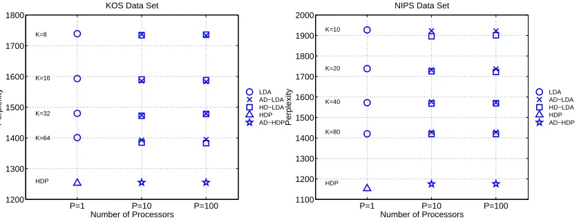
4.1 Perplexity

The perplexity results for KOS and NIPS in Figure 5 clearly show that the model perplexity is essentially the same for the distributed models AD-LDA and AD-HDP at P=10 and P=100 as their single-processor versions at P=1. The figures show the test set perplexity, versus number of processors, P, for different numbers of topics K for the LDA-type models, and also for the HDP-models which learn the number of topics. The P=1 perplexity is computed by LDA (circles) and HDP (triangles), and we use our distributed algorithms—AD-LDA (crosses), HD-LDA (squares), and AD-HDP (stars)—to compute the P=10 and P=100 perplexities. The variability in perplexity as a function of the number of topics is much greater than the variability due to the number of processors. Note that there is essentially no perplexity difference between AD-LDA and HD-LDA.

P=1 P=10 P=100

1200 1300 1400 1500 1600 1700 1800

Number of Processors

Perplexity

KOS Data Set

K=8 K=16 K=32 K=64 HDP LDA AD−LDA HD−LDA HDP AD−HDP

P=1 P=10 P=100

1100 1200 1300 1400 1500 1600 1700 1800 1900 2000

Number of Processors

Perplexity

NIPS Data Set

K=10 K=20 K=40 K=80 HDP LDA AD−LDA HD−LDA HDP AD−HDP

Figure 5: Test perplexity on KOS (left) and NIPS (right) data versus number of processors P. P=1 corresponds to LDA and HDP. At P=10 and P=100 we show AD-LDA, HD-LDA and AD-HDP.

100 101 102 103 104 1350

1400 1450 1500 1550 1600 1650 1700 1750

T=8

T=16

T=32

T=64

Number of processors P

Perplexity

KOS Data Set

100 101 102 103 104

1400 1500 1600 1700 1800 1900 2000

T=10

T=20

T=40

T=80

Number of processors P

Perplexity

NIPS Data Set

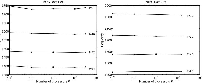
Figure 6: AD-LDA test perplexity versus number of processors up to the limiting case of number of processors equal to number of documents in collection. Left plot shows perplexity for KOS and right plot shows perplexity for NIPS.

AD-HDP instantiates fewer topics but produces a similar perplexity to HDP. The average num-ber of topics instantiated by HDP on KOS was 669 while the average numnum-ber of topics instantiated by AD-HDP was 490 (P=10) and 471 (P=100). For NIPS, HDP instantiated 687 topics while AD-HDP instantiated 569 (P=10) and 569 (P=100) topics. AD-HDP instantiates fewer topics because of the merging across processors of newly-created topics. The similar perplexity results for AD-HDP compared to HDP, despite the fewer topics, is partly due to the relatively small probability mass in many of the topics.

Despite no formal convergence guarantees, the approximate distributed algorithms, AD-LDA and AD-HDP, converged to good solutions in every single experiment (of the more than one hun-dred) we conducted using multiple real-world data sets. We also tested both our distributed LDA algorithms with adversarial/non-random distributions of topics across processors using synthesized data. One example of an adversarial distribution of documents is where each document only uses a single topic, and these documents are distributed such that processor p only has documents that are about topic p. In this case the distributed topic models have to learn the correct set of P topics, even though each processor only sees local documents that pertain to just one of the topics. We ran mul-tiple experiments, starting with 1000 documents that were hard-assigned to K=10 topics (i.e., each document is only about one topic), and distributing the 1000 documents over P=10 processors, where each processor contained documents belonging to the same topic (an analogy is one proces-sor only having documents about sports, the next procesproces-sor only having documents about arts, and so on). The perplexity performance of AD-LDA and HD-LDA under these adversarial/non-random distribution of documents was as good as the performance when the documents were distributed randomly, and as good as the performance of single-processor LDA.

To demonstrate that the low perplexities obtained from the distributed algorithms with P=

higher than the P=100 test perplexity of 1575 for AD-LDA and HD-LDA. This shows that a baseline approach of simple averaging of results from separate processors performs much worse than the distributed coordinated learning algorithms that we propose in this paper.

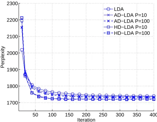
4.2 Convergence

One could imagine that distributed algorithms, where each processor only sees its own local data, may converge more slowly than single-processor algorithms where the data is global. Consequently, we performed experiments to see whether our distributed algorithms were converging at the same rate as their sequential counterparts. If the distributed algorithms were converging slower, the com-putational gains of parallelization would be reduced. Our experiments consistently showed that the convergence rate for the distributed LDA algorithms was just as fast as those for the single processor case. As an example, Figure 7 shows test perplexity versus iteration of the Gibbs sampler for the NIPS data at K=20 topics. During burn-in, up to iteration 200, the distributed algorithms are ac-tually converging slightly faster than single processor LDA. Note that one iteration of AD-LDA or HD-LDA on a parallel multi-processor computer only takes a fraction (at best 1_P) of the wall-clock time of one iteration of LDA on a single processor computer.

50 100 150 200 250 300 350 400 1700

1800 1900 2000 2100 2200 2300

Iteration

Perplexity

LDA

AD−LDA P=10 AD−LDA P=100 HD−LDA P=10 HD−LDA P=100

Figure 7: Convergence of test perplexity versus iteration for the distributed algorithms AD-LDA and HD-LDA using the NIPS data set and K=20 topics.

is ultimately producing a model that has the same predictive ability as HDP. We observe a similar result for the NIPS data set.

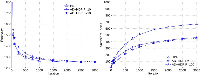
One way to accelerate the rate of convergence for AD-HDP is to match newly generated topics by similarity instead of by topic-id. Figure 9 shows that performing the greedy matching scheme for new topics as described in Algorithm 4 significantly improves the rate of convergence for AD-HDP. In this experiment, we used a threshold of 2 for determining topic similarity. The number of topics increases at a faster rate for AD-HDP with matching, since the greedy matching scheme is more flexible in that the number of new topics at each iteration is not limited to the maximum number of new topics instantiated on any one processor. The results show that the greedy matching scheme enables AD-HDP P=100 to converge almost as quickly as HDP. In practice, only a few new topics are generated locally on each processor each iteration, and so the computational overhead of this heuristic matching scheme is minimal relative to the time for Gibbs sampling.

0 500 1000 1500 2000 2500 3000

1200 1300 1400 1500 1600 1700 1800

Iteration

Perplexity

HDP AD−HDP P=10 AD−HDP P=100

0 500 1000 1500 2000 2500 3000

0 100 200 300 400 500 600 700 800 900 1000

Iteration

Number of Topics

HDP AD−HDP P=10 AD−HDP P=100

Figure 8: Results for HDP versus AD-HDP with no matching. Left plot shows test perplexity versus iteration for HDP and AD-HDP. Right plot shows number of topics versus iteration for HDP and AD-HDP. Results are for the KOS data set.

To further check that the distributed algorithms were performing comparably to their single processor counterparts, we ran experiments to investigate whether the results were sensitive to the number of topics used in the models, in case the distributed algorithms’ performance worsens when the number of topics becomes very large. Figure 10 shows the test perplexity computed on the NIPS data set, as a function of the number of topics, for the LDA algorithms and a fixed number of processors P=10 (the results for the KOS data set were quite similar and therefore not shown). The perplexities of the different algorithms closely track each other as number of topics, K, increases. In fact, in some cases HD-LDA produces slightly lower perplexities than those of single processor LDA. This lower perplexity may be due to the fact that in HD-LDA test perplexity is computed using P sets of topic parameters, thus it has more parameters than AD-LDA to better fit the data.

4.3 Precision and Recall

0 500 1000 1500 2000 2500 3000 1200

1300 1400 1500 1600 1700 1800

Iteration

Perplexity

HDP AD−HDP P=100

AD−HDP P=100 (with matching)

0 500 1000 1500 2000 2500 3000

0 100 200 300 400 500 600 700 800 900 1000

Iteration

Number of Topics

HDP AD−HDP P=100

AD−HDP P=100 (with matching)

Figure 9: Results for HDP versus AD-HDP with greedy matching. Left plot shows test perplexity versus iteration for HDP and AD-HDP. Right plot shows number of topics versus iteration for HDP and AD-HDP. Results are for the KOS data set.

0 100 200 300 400 500 600 700

1000 1100 1200 1300 1400 1500 1600 1700 1800 1900 2000

Number of Topics

Perplexity

LDA AD−LDA P=10 HD−LDA P=10

Figure 10: Test perplexity versus number of topics using the NIPS data set (S=5).

the model is learned, each test document can be treated as a ”query”, where the goal is to retrieve relevant documents from the training set. For each test document, the training documents are ranked according to how probable the test document is under each training document’s mixtureθj and the

set of topics φ. From this ranking, one can calculate mean average precision and area under the ROC curve.

0 10 20 30 40 50 0.04

0.06 0.08 0.1 0.12 0.14 0.16

Iteration

Mean Average Precision

LDA AD−LDA P=10 AD−LDA P=100

0 10 20 30 40 50 0.5

0.55 0.6 0.65 0.7 0.75 0.8 0.85 0.9

Iteration

Mean Area Under ROC Curve

LDA AD−LDA P=10 AD−LDA P=100

Figure 11: Precision/recall results: (left) Mean average precision for LDA/AD-LDA. (right) Area under the ROC curve for LDA/AD-LDA.

5. Scalability

The primary motivation for developing distributed algorithms for LDA and HDP is to have highly scalable algorithms, in terms of memory and computation time. Memory requirements depend on both memory for data and memory for model parameters. The memory for the data scales with N, the total number of words in the corpus. The memory for the parameters is linear in the number of topics K, which is either fixed for the LDA models or learned for the HDP models. The per-processor per-iteration time and space complexity of LDA and AD-LDA are shown in Table 3. AD-LDA’s memory requirement scales well as collection sizes grow, because while corpus size (N and D) can get arbitrarily large, which can be offset by increasing the number of processors, P, the vocabulary size W will tend to asymptote, or at least grow more slowly. Similarly the time complexity scales well since the leading order term NK is divided by P.

The communication cost of the reduce operation, denoted by C in the table, represents the time taken to perform the global sum of the count difference∑_p(Nwk p−Nwk). This is executed in log P

stages and can be implemented efficiently in standard language/protocols such as MPI, the Message Passing Interface. Because of the additional KW term, parallel efficiency will depend on _PWN , with increasing efficiency as this ratio increases. Space and time complexity of HD-LDA are similar to that of AD-LDA, but HD-LDA has bigger constants. For a given number of topics, K, we argue that AD-HDP has similar time complexity as AD-LDA.

We performed large-scale speedup experiments with just AD-LDA instead of all three of our distributed topic modeling algorithms because AD-LDA produces very similar results to HD-LDA, but with significantly less computation. We expect that relative speedup performance for HD-LDA and AD-HDP should follow that for AD-LDA.

LDA AD-LDA

Space N+K(D+W) _P1(N+KD) +KW

Time NK _P1NK+KW+C

0 200 400 600 800 1000 0

100 200 300 400 500 600 700 800 900 1000

Number of processors

Speedup

Perfect

AD−LDA (PUBMED) AD−LDA (WIKIPEDIA)

Figure 12: Parallel speedup results for 64 to 1024 processors on multi-million document data sets WIKIPEDIA and PUBMED.

We used two multi-million document data sets, WIKIPEDIA and PUBMED, for speedup exper-iments on a large-scale supercomputer. The supercomputer used was DataStar, a 15.6 TFlop teras-cale machine at San Diego Supercomputer Center built from 265 IBM P655 8-way compute nodes. We implemented a parallel version of AD-LDA using the Message Passing Interface protocol. We ran AD-LDA on WIKIPEDIA using K=1000 topics and PUBMED using K =2000 topics dis-tributed over P=64,128,256,512 and 1024 processors. The speedup results, shown in Figure 12, show relatively high parallel efficiency, with approximately 700 times speedup for WIKIPEDIA and 800 times speedup for PUBMED when using P=1024 processors, corresponding to parallel efficiencies of approximately 0.7 and 0.8 respectively. This speedup is computed relative to the time per iteration when using P=64 processors (i.e., at P=64 processors speedup=64), since it is not possible, due to memory limitations, to run these models on a single processor. Multiple runs were timed for both WIKIPEDIA and PUBMED, and the resulting variation in timing was less than 1%, so error bars are not shown in the figure. We see slightly higher parallel efficiency for PUBMED versus WIKIPEDIA because PUBMED has a larger amount of computation per unit data communicated, _PWN .

In addition to the large-scale speedup experiments run on the 1024-processor parallel super-computer, we also performed small-scale speedup experiments for AD-HDP on an 8-node parallel cluster running MPI. Using the NIPS data set we measured parallel efficiencies of 0.75 and 0.5 for

P=4 and P=8. The latter result on 8 processors means that the HDP model for NIPS can be learned four times faster than on a single processor.

6. Analysis of Approximate Distributed LDA

Finally, we investigate the dynamics of AD-LDA learning using toy data to get further insight into how AD-LDA is working. While we have shown experimental results showing that AD-LDA produces models with similar perplexity and similar convergence rates to LDA, it is not obvious why this algorithm works so well in practice. Our toy example has W =3 words and K=2 topics. We generated document collections according to the LDA generative process given by (1). We chose a low dimension vocabulary, W , so that we could plot the evolution of the Gibbs sampler on a two-dimensional word-topic simplex. We first generated data, then learned models using LDA and AD-LDA.

The left plot of Figure 13 shows the L1 distance between the model’s estimate of a particular

topic-word distribution and the true distribution, as a function of Gibbs iteration, for both single-processor LDA and AD-LDA with P=2. LDA and AD-LDA have qualitatively the same three-phase learning dynamics. The first four or so iterations (labeled initialize) correspond to somewhat random movement close to the randomly initialized starting point. In the next phase (labeled

burn-in) both algorithms rapidly move in parameter space toward the posterior mode. And finally after

burn-in (labeled stationary) both are sampling around the mode. In the right plot we show the sim-ilarity between AD-LDA and LDA samples taken from the equilibrium distribution—here plotted on the two-dimensional planar simplex corresponding to the three-word topic distribution.

0 20 40 60 80 100

0 0.05 0.1 0.15 0.2 0.25 0.3 0.35 0.4

Iteration

L1 norm

initialize

burn−in

stationary

LDA

AD−LDA proc1 AD−LDA proc2

0.8 0.81 0.82 0.83 0.84 0.85

0.445 0.45 0.455 0.46 0.465 0.47 0.475

topic mode

LDA AD−LDA

Figure 13: (Left) L1distance to the mode for LDA and for P=2 AD-LDA. (Right) Closeup of 50

samples ofφ(projected onto the topic simplex) taken from the equilibrium distribution, showing the similarity between LDA and P=2 AD-LDA. Note the zoomed scale in this figure.

learning dynamics: taking a few small steps near the starting point, moving up to the true solution, and then sampling near the posterior mode for the rest of the iterations. For each Gibbs iteration, the parameters corresponding to each of the two individual processors, and those parameters after merging, are shown for AD-LDA. One can see the alternating pattern of two separate (but close) parameter estimates on each processor, followed by a merged estimate. We observed that after the initial few iterations, the individual processor steps and the merge step each resulted in a move closer to the mode. One might worry that the AD-LDA algorithm would get trapped close to the initial starting point, for example, due to repeated label switching or oscillatory behavior of topic labeling across processors. In practice we have consistently observed that the algorithm quickly discards such configurations due to the stochastic nature of the moves and latches onto a consistent and stable labeling that rapidly moves it toward the posterior mode. The figure clearly illustrates that LDA and AD-LDA have qualitatively similar learning dynamics. The right plot in Figure 14 illustrates the same qualitative behavior as in the left plot, but now for P=10 processors.

Interestingly, across a wide range of experiments, we observed that the variance in the AD-LDA word-topic distribution samples is typically only about 70% of the variance in AD-LDA topic samples. Since the samplers are not the same it makes sense that the posterior variance differs (i.e., is underestimated) by the parallel sampler. We expect less variance because AD-LDA ignores fluctuations in the bulk of Nwk. Nonetheless, all of our experiments indicate that the posterior mode

and means found by the parallel sampler are essentially the same as those found by the sequential sampler.

0.65 0.7 0.75 0.8 0.85 0.9

0.36 0.38 0.4 0.42 0.44 0.46 0.48 0.5

start

topic mode

LDA

AD−LDA proc1 AD−LDA proc2

0.65 0.7 0.75 0.8 0.85 0.9

0.36 0.38 0.4 0.42 0.44 0.46 0.48 0.5

start

topic mode

LDA

AD−LDA proc1 AD−LDA proc2 AD−LDA proc3 ...etc... AD−LDA proc10

Figure 14: (Left) Projection of topics onto simplex, showing convergence to mode for P =2. (Right) Same as left plot, but with P=10.

100 101 102 103 104 0

0.01 0.02 0.03 0.04 0.05 0.06 0.07 0.08 0.09

Number of processors, P

||

E(

φ

)−

φ ref

||

reference = LDA reference = true

Figure 15: Average L1error in word-topic distribution versus P for AD-LDA.

While we see similar perplexities for AD-LDA compared to LDA, we could further ask if the AD-LDA algorithm is producing any bias in its estimates of the model parameters. To test this, we performed a series of experiments where we generated synthetic data sets according to the LDA generative process, with known word-topic distributionsφ∗. We then learned LDA and AD-LDA models from each of the simulated data sets. We computed the expected value of the AD-LDA top-ics E(φ)and compared this to two reference values,φrefone based on the true distribution,φref=φ∗,

the other based on multiple LDA samples,φref=E[φLDA]. Figure 15 shows that AD-LDA is much

closer to the LDA topics E[φLDA]than either are to the true topicsφ∗, telling us that the sampling

variation in learning LDA models from finite data sets is much greater than the variation between LDA and AD-LDA on the same data sets.

6.1 When Does AD-LDA Fail?

In all of our experiments thus far, we have seen that our distributed algorithms learn models with equivalent predictive power as their non-distributed counterparts. However, when global synchro-nizations are done less frequently (i.e., when the synchronization step is performed after multiple Gibbs sampling sweeps through local data), the distributed algorithms may converge to suboptimal solutions.

each processor have the freedom to drift. In contrast, when P=100 processors, each processor can only locally modify 1/100thof the topic assignments, and so the topics on each processor can not drift far from the global set of topic counts at the previous iteration. Bipartite matching significantly improves the perplexity in the P=2 processor case, suggesting that the lack of communication has indeed caused the topics to drift apart. Fortunately, topic drifting becomes less of a problem as more processors are used, and can be eliminated by frequent synchronization. It is also important to note that AD-LDA P=2, where processors synchronize after every iteration, gives essentially identical results as LDA. Our recommendation in practice is to perform the synchronization and count updates after each iteration of the Gibbs sampler. As shown earlier in the paper, this leads to performance that is essentially indistinguishable from LDA. Since most multi-processor comput-ing hardware will tend to have communication bandwidth matched to processor speed (i.e., faster and/or more processors usually come with a faster communication network), synchronizing after each iteration of the Gibbs sampler will usually be the optimal strategy.

0 1000 2000 3000 4000 5000

1700 1800 1900 2000 2100 2200 2300 2400 2500

Iteration

Perplexity

LDA AD−LDA P=2

AD−LDA P=2, Sync=100

AD−LDA P=2, Sync=100 (with matching) AD−LDA P=100, Sync=100

Figure 16: Test perplexity versus iteration where synchronizations between processors only occur every 100 iterations, KOS, K=16.

7. Related Work

the number of distinct document-word pairs in the corpus. For typical English-language corpora, the total number of words in the corpus is less than twice the number of distinct document-word pairs (N <2M), so M can be considered on the order of N. Since M is usually much larger than the number of documents, D, this memory requirement of MK is not nearly as scalable as that the memory requirement of N+DK for MCMC methods.

Parallelized versions of various machine learning algorithms have also been developed. Forman and Zhang (2000) describe a parallel k-means algorithm, and W. Kowalczyk and N. Vlassis (2005) describe an asynchronous parallel EM algorithm for Gaussian mixture learning. A parallel EM algorithm for Probabilistic Latent Semantic Analysis, implemented using Google’s MapReduce framework, was described in Das et al. (2007). A review of how to parallelize an array of standard machine learning algorithms using MapReduce was presented by Chu et al. (2007). Rossini et al. (2007) presents a framework for statisticians that allows for the parallel computing of independent tasks within the R language.

While many of these EM algorithms are readily parallelizable, Gibbs sampling of dependent variables (such as topic assignments) is fundamentally sequential and therefore difficult to paral-lelize. One way to parallelize Gibbs sampling is to run multiple independent chains in parallel to obtain multiple samples; however, this multiple-chain approach does not address the fact that the burn-in within each chain may take a long time. Furthermore, for some applications, one is not in-terested in multiple samples from independent chains. For example, if we wish to learn topics for a very large document collection, one is usually satisfied with mean values of word-topic distributions taken from a single chain.

One can parallelize a single MCMC chain by decomposing the variables into independent non-interacting blocks that can be sampled concurrently (Kontoghiorghes, 2005). However, when the variables are not independent, sampling variables in parallel is not possible. Brockwell (2006) presents a general parallel MCMC algorithm based on pre-fetching, but it is not practical for learning topic models because it discards most of its computations which makes it relatively inefficient. It is possible to construct partially parallel Gibbs samplers, in which the samples are independently accepted with some probability. In the limit as this probability goes to zero, this sampler will approach the sequential Gibbs sampler, as explained in P. Ferrari et al. (1993). However, this method is also not practical when learning topic models because it is computationally inefficient. Younes (1998) shows the existence of exact parallel samplers that make use of periodic synchronous random fields. However there is no known method for constructing such a sampler.

8. Conclusions

We have proposed three different algorithms for distributing across multiple processors Gibbs sam-pling for LDA and HDP. With our approximate distributed algorithm, AD-LDA, we sample from an approximation to the posterior distribution by allowing different processors to concurrently sample topic assignments on their local subsets of the data. Despite having no formal convergence guar-antees, AD-LDA works very well empirically and is easy to implement. With our hierarchical dis-tributed model, HD-LDA, we adapt the underlying LDA model to map to the disdis-tributed processor architecture. This model is more complicated than AD-LDA, but it inherits the usual convergence properties of Markov chain Monte Carlo. We discovered that careful selection of hyperparameters was critical to making HD-LDA work well, but this selection was clearly informed by AD-LDA. Our distributed algorithm AD-HDP followed the same approach as AD-LDA, but with an additional step to merge newly instantiated topics.

Our proposed distributed algorithms learn LDA models with predictive performance that is no different than single-processor LDA. On each processor they burn-in and converge at the same rate as LDA, yielding significant speedups in practice. For HDP, our distributed algorithm eventually produced the same perplexity as the single-processor version of HDP. Prior to reaching the con-verged perplexity result, AD-HDP had higher perplexity than HDP since the merging of new topics by label slows the rate of topic growth. We also discovered that matching new topics by similarity significantly improves AD-HDP’s rate of convergence.

The space and time complexity of these distributed algorithms make them scalable to run very large data sets, for example, collections with billions to trillions of words. Using two multi-million document data sets, and running computations on a 1024-processor parallel supercomputer, we showed how one can achieve a 700-800 times reduction in wall-clock time by using our distributed approach.

There are several potentially interesting research directions that can be pursued using the algo-rithms proposed here as a starting point. One research direction is to use more complex schemes that allow data to adaptively move from one processor to another. The distributed schemes presented in this paper can also be used to parallelize topic models that are based on or derived from LDA and HDP, and beyond that a potentially larger class of graphical models.

Acknowledgments

Appendix A.

The auxiliary variable method explained in Escobar and West (1995) and Teh et al. (2006) is used to sampleα,β, andΦ. To derive Gibbs sampling equations, we use the following expansions:

Γ(u) Γ(u+n) =

1

Γ(n)B(u,n) =

1

Γ(n) Z 1

0 t

u−1_(1−t)n−1_{dt (8)} Γ(u+n)

Γ(u) = n

∑

S(n,s)(u)s (S is Stirling number of first kind) (9)

The first expansion follows from the definition of the Beta function, and the second expansion makes use of the Stirling number of the first kind to rewrite the factorial (see Abramowitz and Stegun, 1964).

Now we derive the sampling equation forαp. Combining the collapsed distribution (6) with the

prior onαp(5) gives the posterior distribution forαp:1

P(αp| )∝

∏

"

Γ(Kαp) Γ(Nj p+Kαp)

∏

Γ(Nk j p+αp) Γ(αp)

#

αc−1 p e−dαp.

Using the expansions (8,9) we introduce the auxiliary variables t and s:

P(αp,t,s| )∝

"

∏

tK_jαp−1(1−tj)Nj p−1_dt

j

# "

∏

∏

S(Nk j p,sk j p)αsk j p

p

#

αc−1 p e−dαp.

The joint distribution above allows us to create sampling equations forαp, t, and s:

P(αp|t,s, )∝

"

∏

tKαp

j

# "

∏

∏

αsk j p

p

#

αc−1 p e−dαp

=Gamma

"

c+

∑

∑

sk j p; d−K

∑

log(tj)

#

,

P(tj|αp,s, )∝t_jKαp−1(1−tj)Nj p−1 =Beta[Kαp,Nj p],

P(sk j p|αp,t, )∝S(Nk j p,sk j p)α sk j p

p =Antoniak[Nk j p,αp].

The Antoniak distribution is the distribution of the number of occupied tables if Nk j pcustomers

are sent into a restaurant that follows the Chinese restaurant process with strength parameterαp.

Sampling from the Antoniak distribution is done by sampling Nk j pBernoulli variables:

sl_{k j p}∼Bernoulli

α

p αp+l−1

l=1. . .Nk j p,

sk j p=

∑

sl_{k j p}.

Using the same auxiliary variable techniques, we derive sampling equations forβandΦ. These variables are sampled jointly because they are dependent. The posterior distribution forβ andΦ and the joint distribution with the auxiliary variables t and s are given by:

P(βk,Φk|)∝

∏

Γ

(βk) Γ(Nk p+βk)

∏

Γ(Nwk p+βkΦw|k) Γ(βkΦw|k)

∏

Φγ−1 w|k

βa−1 k e−

bβk_,

P(βk,Φk,t,s|)∝

"

∏

tβk−1

k p (1−tk p) Nk p−1

# "

∏

∏

S(Nwk p,swk p)(βkΦw|k)swk p

#

"

∏

∏

Φγ−1 w|k

#

βa−1 k e

−bβk_.

Note that the set of variables (t and s) is unrelated to the set of auxiliary variables introduced for

αp. The sampling equations forβ,Φ, t, and s are:

P(βk|Φ,t,s, )∝

"

∏

tβk

k p

# "

∏

∏

(βk)swk p

#

βa−1 k e

−bβk

=Gamma

"

a+

∑

∑

swk p; b−

∑

p

log(tk p)

#

,

P(Φk|βk,t,s, )∝

"

∏

∏

Φswk p

w|k

#

∏

Φγ−1 w|k

=Dirichlet "

γ+

∑

swk p

#

,

P(tk p|βk,Φk,s, )∝tk pβk−1(1−tk p)Nk p−1 =Beta[βk,Nk p],

P(swk p|βk,Φk,t, )∝S(Nwk p,swk p)(βkΦw|k)swk p =AntoniakNwk p,βkΦw|k

.

References

M. Abramowitz and I. Stegun. Handbook of Mathematical Functions with Formulas, Graphs, and

A. Asuncion and D. Newman. UCI machine learning repository, 2007. URL http://www.ics.uci.edu/∼mlearn/MLRepository.html.

D. Blei, A. Ng, and M. Jordan. Latent Dirichlet allocation. In Advances in Neural Information

Processing Systems, volume 14, pages 601–608, Cambridge, MA, 2002. MIT Press.

D. Blei, A. Ng, and M. Jordan. Latent Dirichlet allocation. Journal of Machine Learning Research, 3:993–1022, 2003.

A. Brockwell. Parallel Markov chain Monte Carlo simulation by pre-fetching. Journal of

Compu-tational & Graphical Statistics, 15, No. 1:246–261, 2006.

R. Burkard and E. C¸ ela. Linear assignment problems and extensions. In P. Pardalos and D. Du, ed-itors, Handbook of Combinatorial Optimization, Supplement Volume A. Kluwer Academic Pub-lishers, 1999.

G. Casella and C. Robert. Rao-Blackwellisation of sampling schemes. Biometrika, 83(1):81–94, 1996.

C. Chemudugunta, P. Smyth, and M. Steyvers. Modeling general and specific aspects of documents with a probabilistic topic model. In Advances in Neural Information Processing Systems 19, pages 241–248. MIT Press, Cambridge, MA, 2007.

Chu, Kim, Lin, Yu, Bradski, Ng, and Olukotun. Map-reduce for machine learning on multicore. In B. Sch¨olkopf, J. Platt, and T. Hoffman, editors, Advances in Neural Information Processing

Systems 19, pages 281–288. MIT Press, Cambridge, MA, 2007.

A. Das, M. Datar, A. Garg, and S. Rajaram. Google news personalization: Scalable online collabo-rative filtering. In WWW ’07: Proceedings of the 16th International Conference on World Wide

Web, pages 271–280, New York, NY, 2007. ACM.

M. D. Escobar and M. West. Bayesian density estimation and inference using mix-tures. Journal of the American Statistical Association, 90(430):577–588, 1995. URL citeseer.ist.psu.edu/escobar94bayesian.html.

G. Forman and B. Zhang. Distributed data clustering can be efficient and exact. In ACM KDD

Explorations, volume 2, pages 34–38, New York, NY, 2000. ACM.

T. Griffiths and M. Steyvers. Finding scientific topics. In Proceedings of the National Academy of

Sciences, volume 101, pages 5228–5235, 2004.

E. Kontoghiorghes. Handbook of Parallel Computing and Statistics (Statistics, Textbooks and Monographs). Chapman & Hall / CRC, 2005.

W. Li and A. McCallum. Pachinko allocation: DAG-structured mixture models of topic correlations. In Proceedings of the International Conference on Machine Learning, volume 23, pages 577–584, New York, NY, 2006. ACM.

D. Mimno and A. McCallum. Organizing the OCA: Learning faceted subjects from a library of digital books. In JCDL ’07: Proceedings of the 2007 conference on digital libraries, pages 376–385, New York, NY, 2007. ACM.

R. Nallapati, W. Cohen, and J. Lafferty. Parallelized variational EM for latent Dirichlet allocation: An experimental evaluation of speed and scalability. In ICDMW ’07: Proceedings of the Seventh

IEEE International Conference on Data Mining Workshops, pages 349–354, Washington, DC,

2007. IEEE Computer Society.

P. Ferrari, A. Frigessi, and R. Schonmann. Convergence of some partially parallel Gibbs samplers with annealing. In Annals of Applied Probability, volume 3, pages 137–153. Institute of Mathe-matical Statistics, 1993.

M. Rosen-Zvi, T. Griffiths, M. Steyvers, and P. Smyth. The author-topic model for authors and documents. In Proceedings of the Conference on Uncertainty in Artificial Intelligence, volume 20, pages 487–494, Arlington, VA, 2004. AUAI Press.

A. Rossini, L. Tierney, and N. Li. Simple parallel statistical computing in R. Journal of

Computa-tional & Graphical Statistics, 16(2):399, 2007.

Y. W. Teh, M. I. Jordan, M. J. Beal, and D. M. Blei. Hierarchical Dirichlet processes. Journal of

the American Statistical Association, 101(476):1566–1581, 2006.

W. Kowalczyk and N. Vlassis. Newscast EM. In Advances in Neural Information Processing

Systems 17, pages 713–720. MIT Press, Cambridge, MA, 2005.

J. Wolfe, A. Haghighi, and D. Klein. Fully distributed EM for very large datasets. In Proceedings

of the International Conference on Machine Learning, pages 1184–1191. ACM, New York, NY,

2008.

L. Younes. Synchronous random fields and image restoration. IEEE Transactions on Pattern