An Extension on “Statistical Comparisons of Classifiers over Multiple
Data Sets” for all Pairwise Comparisons
Salvador Garc´ıa [email protected]
Francisco Herrera [email protected]
Department of Computer Science and Artificial Intelligence University of Granada
Granada, 18071, Spain
Editor: John Shawe-Taylor
Abstract
In a recently published paper in JMLR, Demˇsar (2006) recommends a set of non-parametric sta-tistical tests and procedures which can be safely used for comparing the performance of classifiers over multiple data sets. After studying the paper, we realize that the paper correctly introduces the basic procedures and some of the most advanced ones when comparing a control method. How-ever, it does not deal with some advanced topics in depth. Regarding these topics, we focus on more powerful proposals of statistical procedures for comparing n×n classifiers. Moreover, we illustrate an easy way of obtaining adjusted and comparable p-values in multiple comparison procedures.
Keywords: statistical methods, non-parametric test, multiple comparisons tests, adjusted p-values,
logically related hypotheses
1. Introduction
In the Machine Learning (ML) scientific community there is a need for rigorous and correct statisti-cal analysis of published results, due to the fact that the development or modifications of algorithms is a relatively easy task. The main inconvenient related to this necessity is to understand and study the statistics and to know the exact techniques which can or cannot be applied depending on the situation, that is, type of results obtained. In a recently published paper in JMLR by Demˇsar (2006), a group of useful guidelines are given in order to perform a correct analysis when we compare a set of classifiers over multiple data sets. Demˇsar recommends a set of non-parametric statistical techniques (Zar, 1999; Sheskin, 2003) for comparing classifiers under these circumstances, given that the sample of results obtained by them does not fulfill the required conditions and it is not large enough for making a parametric statistical analysis. He analyzed the behavior of the pro-posed statistics on classification tasks and he checked that they are more convenient than parametric techniques.
ensembles of decision trees, non-parametric tests are also applied in the analysis of performance (Banfield et al., 2007). However, only the rankings computed by Friedman’s method (Friedman, 1937) are stipulated and authors establish comparisons based on them, without taking into account significance levels. Demˇsar focused his work in the analysis of new proposals, and he introduced the Nemenyi test for making all pairwise comparisons (Nemenyi, 1963). Nevertheless, the Nemenyi test is very conservative and it may not find any difference in most of the experimentations. In recent papers, the authors have used the Nemenyi test in multiple comparisons. Due to the fact that this test posses low power, authors have to employ many data sets (Yang et al., 2007b) or most of the differences found are not significant (Yang et al., 2007a; N ´u˜nez et al., 2007). Although the employment of many data sets could seem beneficial in order to improve the generalization of results, in some specific domains, that is, imbalanced classification (Owen, 2007) or multi-instance classification (Murray et al., 2005), data sets are difficult to find.
Procedures with more power than Nemenyi’s one can be found in specialized literature. We have based on the necessity to apply more powerful procedures in empirical studies in which no new method is proposed and the benefit consists of obtaining more statistical differences among the classifiers compared. Thus, in this paper we describe these procedures and we analyze their behavior by means of the analysis of multiple repetitions of experiments with randomly selected data sets.
On the other hand, we can see other works in which the p-value associated to a comparison between two classifiers is reported (Garc´ıa-Pedrajas and Fyfe, 2007). Classical non-parametric tests, such as Wilcoxon and Friedman (Sheskin, 2003), may be incorporated in most of the statistical packages (SPSS, SAS, R, etc.) and the computation of the final p-value is usually implemented. However, advanced procedures such as Holm (1979), Hochberg (1988), Hommel (1988) and the ones described in this paper are usually not incorporated in statistical packages. The computation of the correct p-value, or Adjusted P-Value (APV) (Westfall and Young, 2004), in a comparison using any of these procedures is not very difficult and, in this paper, we show how to include it with an illustrative example.
The paper is set up as follows. Section 2 presents more powerful procedures for comparing all the classifiers among them in a n×n comparison of multiple classifiers and a case study. In Section 3 we describe the procedures for obtaining the APV by considering the post-hoc procedures explained by Demˇsar and the ones explained in this paper. In Section 4, we perform an experimental study of the behavior of the statistical procedures and we discuss the results obtained. Finally, Section 5 concludes the paper.
2. Comparison of Multiple Classifiers: Performing All Pairwise Comparisons
ones. For this reason, he described and studied in depth more powerful and sophisticated procedures derived from Bonferroni-Dunn such as Holm’s, Hochberg’s and Hommel’s methods.
Nevertheless, we think that performing all pairwise comparisons in an experimental analysis may be useful and interesting in different cases when proposing a new method. For example, it would be interesting to conduct a statistical analysis over multiple classifiers in review works in which no method is proposed. In this case, the repetition of comparisons choosing different control classifiers may lose the control of the family-wise error.
Our intention in this section is to give a detailed description of more powerful and advanced procedures derived from the Nemenyi test and to show a case study that uses these procedures.
2.1 Advanced Procedures for Performing All Pairwise Comparisons
A set of pairwise comparisons can be associated with a set or family of hypotheses. Any of the post-hoc tests which can be applied to non-parametric tests (that is, those derived from the Bonferroni correction or similar procedures) work over a family of hypotheses. As Demˇsar explained, the test statistics for comparing the i-th and j-th classifier is
z=(qRi−Rj)
k(k+1)
6N ,
where Ri is the average rank computed through the Friedman test for the i-th classifier, k is the number of classifiers to be compared and N is the number of data sets used in the comparison.
The z value is used to find the corresponding probability (p-value) from the table of normal dis-tribution, which is then compared with an appropriate level of significanceα(Table A1 in Sheskin, 2003). Two basic procedures are:
• Nemenyi (1963) procedure: it adjusts the value ofαin a single step by dividing the value of
αby the number of comparisons performed, m=k(k−1)/2. This procedure is the simplest but it also has little power.
• Holm (1979) procedure: it was also described in Demˇsar (2006) but it was used for compar-isons of multiple classifiers involving a control method. It adjusts the value ofα in a step down method. Let p1, ...,pmbe the ordered p-values (smallest to largest) and H1, ...,Hm be the corresponding hypotheses. Holm’s procedure rejects H1to H(i−1)if i is the smallest
in-teger such that pi>α/(m−i+1). Other alternatives were developed by Hochberg (1988), Hommel (1988) and Rom (1990). They are easy to perform, but they often have a similar power to Holm’s procedure (they have more power than Holm’s procedure, but the difference between them is not very notable) when considering all pairwise comparisons.
Based on this argument, Shaffer proposed two procedures which make use of the logical relation among the family of hypotheses for adjusting the value ofα(Shaffer, 1986).
• Shaffer’s static procedure: following Holm’s step down method, at stage j, instead of rejecting Hiif pi≤α/(m−i+1), reject Hiif pi≤α/ti, where tiis the maximum number of hypotheses which can be true given that any(i−1)hypotheses are false. It is a static procedure, that is, t1, ...,tmare fully determined for the given hypotheses H1, ...,Hm, independent of the observed p-values. The possible numbers of true hypotheses, and thus the values of ti can be obtained from the recursive formula
S(k) = k [
j=1 {
j 2
+x : x∈S(k−j)},
where S(k)is the set of possible numbers of true hypotheses with k classifiers being compared, k≥2, and S(0) =S(1) ={0}.
• Shaffer’s dynamic procedure: it increases the power of the first by substitutingα/ti at stage i by the valueα/t∗
i, where ti∗ is the maximum number of hypotheses that could be true, given that the previous hypotheses are false. It is a dynamic procedure since ti∗ depends not only on the logical structure of the hypotheses, but also on the hypotheses already rejected at step i. Obviously, this procedure has more power than the first one. In this paper, we have not used this second procedure, given that it is included in an advanced procedure which we will describe in the following.
In Bergmann and Hommel (1988) was proposed a procedure based on the idea of finding all elementary hypotheses which cannot be rejected. In order to formulate Bergmann-Hommel’s pro-cedure, we need the following definition.
Definition 1 An index set of hypotheses I⊆ {1, ...,m}is called exhaustive if exactly all Hj, j∈I, could be true.
In order to exemplify the previous definition, we will consider the following case: We have three classifiers, and we will compare them in a n×n comparison. We will obtain three hypotheses:
• H1= C1es equal in behavior than C2. • H2= C1es equal in behavior than C3. • H3= C2es equal in behavior than C3. and eight possible sets Si:
• S1: All Hjare true.
• S2: H1and H2are true and H3is false.
• S4: H2and H3are true and H1is false.
• S5: H1is true and H2and H3are false. • S6: H2is true and H1and H3are false.
• S7: H3is true and H1and H2are false.
• S8: All Hjare false.
Sets S1, S5, S6, S7and S8can be possible, because their hypotheses can be true at the same time, so they are exhaustive sets. Set S2, basing on logically related hypotheses principles, is not possible because the performance of C1cannot be equal to C2and C3, whereas C2has different performance than C3. The same consideration can be done to S3and S4, which are not exhaustive sets.
Under this definition, it works as follows.
• Bergmann and Hommel (1988) procedure: Reject all Hjwith j∈/A, where the acceptance set
A=[{I : I exhaustive, min{Pi: i∈I}>α/|I|}
is the index set of null hypotheses which are retained.
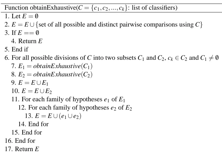
For this procedure, one has to check for each subset I of{1, ...,m}if I is exhaustive, which leads to intensive computation. Due to this fact, we will obtain a set, named E, which will contain all the possible exhaustive sets of hypotheses for a certain comparison. A rapid algo-rithm which was described in Hommel and Bernhard (1994) allows a substantial reduction in computing time. Once the E set is obtained, the hypotheses that do not belong to the A set are rejected.
An example illustrating the algorithm for obtaining all exhaustive sets is drawn in Figure 2. In it, four classifiers, enumerated from 1 to 4 in the C set, are used. The comparisons or hy-potheses are denoted by pairs of numbers without a separation character between them. This illustration does not show the case in which the set|Ci|<2, for simplifying the representation. When|Ci|<2, no comparisons can be performed, so the obtainExhaustive function returns an empty set E.
An edge connecting two boxes represents an invocation of this function. In each box, the list of classifiers given as input and the first initialization of the E set are displayed. The main edges, whose starting point is the initial box, are labeled by the order of invocation. Below the graph, the resulting E subset in each main edge is denoted. The final E will be composed by the union of these E subsets. At the end of the process, 14 distinct exhaustive sets are found: E={(12,13,14,23,24,34),(23,24,34),(13,14,34),(12,14,24),(12,13,23), (12),(13),(14),(23),(24),(34),(12,34),(13,24),(23,14)}.
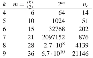
Table 1 gives the number of hypotheses (m), the number (2n) of index sets I and the number of exhaustive index sets (ne) for k classifiers being compared.
Function obtainExhaustive(C={c1,c2, ...,ck}: list of classifiers) 1. Let E=/0
2. E=E∪ {set of all possible and distinct pairwise comparisons using C} 3. If E== /0
4. Return E 5. End if
6. For all possible divisions of C into two subsets C1and C2, ck∈C2and C16= /0 7. E1=obtainExhaustive(C1)
8. E2=obtainExhaustive(C2) 9. E =E∪E1
10. E =E∪E2
11. For each family of hypotheses e1of E1 12. For each family of hypotheses e2of E2
13. E=E∪(e1∪e2) 14. End for
15. End for 16. End for 17. Return E
Figure 1: Algorithm for obtaining all exhaustive sets
The following subsections present a case study of a n×n comparison of some well-known classifiers over thirty data sets. In it, the four procedures explained above are employed.
2.2 Performing All Pairwise Comparisons: A Case Study
C = {1, 2, 3, 4}
E = {(12,13,14,23,24,34)} C2= {1, 2, 3}
E = {(12,13,23)} C1= {1, 2} E = {(12)} C2= {1, 3}
E = {(13)} C2= {2, 3} E = {(23)}
1: E = {(12,13,23),(23),(13),(12)}
2: E = {(12),(34),(12,34)}
3: E = {(13),(24),(13,24)}
4: E = {(23,24,34),(23),(24),(34)}
5: E = {(23),(14),(23,14)}
6: E = {(13,14,34),(13),(14),(34)}
7: E = {(12,14,24),(12),(14),(24)}
C1= {1, 2}
E = {(12)}
C2= {3, 4}
E = {(34)}
C1= {1, 3} E = {(13)}
C2= {2, 4} E = {(24)}
C2= {2, 3, 4} E = {(23,24,34)}
C2= {3, 4} E = {(34)}
C2= {2, 4} E = {(24)} C1= {2, 3} E = {(23)} C1= {1, 4}
E = {(14)} C1= {2, 3}
E = {(23)} C2= {1, 3, 4}
E = {(13,14,34)}
C2= {3, 4} E = {(34)} C2= {1, 4} E = {(14)} C1= {1, 3}
E = {(13)}
C2= {1, 2, 4}
E = {(12,14,24)}
C2= {2, 4} E = {(24)} C2= {1, 4} E = {(14)} C1= {1, 2} E = {(12)}
1 2 3 4 5 6 7
Figure 2: Example of the obtaining of exhaustive sets of hypotheses considering 4 classifiers
k m= k2
2m ne
4 6 64 14
5 10 1024 51
6 15 32768 202
7 21 2097152 876 8 28 2.7·108 4139 9 36 6.7·1010 21146
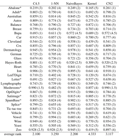
NaiveBayes, Kernel (McLachlan, 2004)1and, finally, CN2 (Clark and Niblett, 1989).2The parame-ters used are specified in Section 4. We have used 10-fold cross validation and standard parameparame-ters for each algorithm. The results correspond to average accuracy or 1−class error in test data. We have used 30 data sets.3 Table 2 shows the overall process of computation of average rankings.
Friedman (1937) and Iman and Davenport (1980) tests check whether the measured average ranks are significantly different from the mean rank Rj =3. They respectively use theχ2and the F statistical distributions to determine if a distribution of observed frequencies differs from the theoretical expected frequencies. Their statistics use nominal (categorical) or ordinal level data, instead of using means and variances. Demˇsar (2006) detailed the computation of the critical values in each distribution. In this case, the critical values are 9.488 and 2.45, respectively atα=0.05, and the Friedman’s and Iman-Davenport’s statistics are:
χ2
F =39.647,FF=14.309.
Due to the fact that the critical values are lower than the respective statistics, we can proceed with the post-hoc tests in order to detect significant pairwise differences among all the classifiers. For this, we have to compute and order the corresponding statistics and p-values. The standard
error in the pairwise comparison between two classifiers is SE=
q
k(k+1)
6N =
q
5·6
6·30 =0.408. Table 3 presents the family of hypotheses ordered by their p-value and the adjustment ofαby Nemenyi’s, Holm’s and Shaffer’s static procedures.
• Nemenyi’s test rejects the hypotheses [1–4] since the corresponding p-values are smaller than the adjustedα’s.
• Holm’s procedure rejects the hypotheses [1–5].
• Shaffer’s static procedure rejects the hypotheses [1–6].
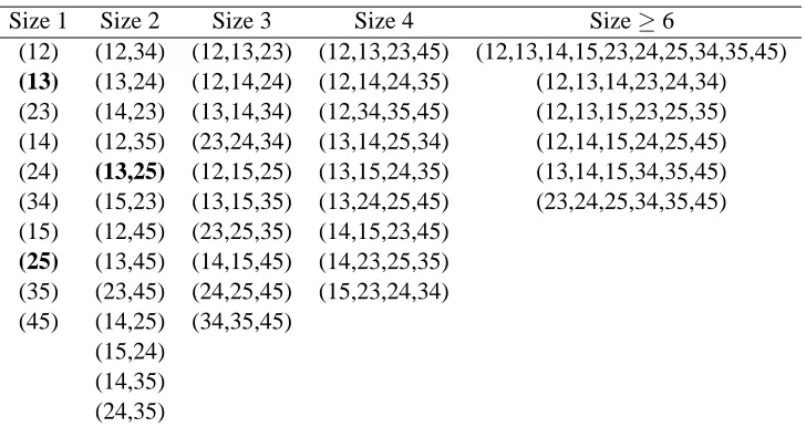
• Bergmann-Hommel’s dynamic procedure first obtains the exhaustive index set of hypotheses. It obtains 51 index sets. We can see them in Table 4. From the index sets, it computes the A set.4 It rejects all hypotheses H
j with j∈/A, so it rejects the hypotheses [1–8].
Bergmann-Hommel’s dynamic procedure allows to clearly distinguishing among three groups of classifiers, attending to their performance:
• Best classifiers: C4.5 and NaiveBayes.
• Middle classifiers: 1-NN and CN2.
• Worst classifier: Kernel.
1. Kernel method is a bayesian classifier which employs a non-parametric estimation of density functions through a gaussian kernel function. The adjustment of the covariance matrix is performed by the ad-hoc method.
2. NaiveBayes and CN2 are classifiers for discrete domains, so we have discretized the data prior to learning with them. The discretizer algorithm is Fayyad and Irani (1993).
3. Data sets marked with ’*’ have been subsampled being adapted to slow algorithms, such as CN2.
C4.5 1-NN NaiveBayes Kernel CN2 Abalone* 0.219 (3) 0.202 (4) 0.249 (2) 0.165 (5) 0.261 (1)
Adult* 0.803 (2) 0.750 (4) 0.813 (1) 0.692 (5) 0.798 (3) Australian 0.859 (1) 0.814 (4) 0.845 (2) 0.542 (5) 0.816 (3) Autos 0.809 (1) 0.774 (3) 0.673 (4) 0.275 (5) 0.785 (2) Balance 0.768 (3) 0.790 (2) 0.727 (4) 0.872 (1) 0.706 (5) Breast 0.759 (1) 0.654 (5) 0.734 (2) 0.703 (4) 0.714 (3) Bupa 0.693 (1) 0.611 (3) 0.572 (4.5) 0.689 (2) 0.572 (4.5)
Car 0.915 (1) 0.857 (3) 0.860 (2) 0.700 (5) 0.777 (4) Cleveland 0.544 (2) 0.531 (4) 0.558 (1) 0.439 (5) 0.541 (3) Crx 0.855 (2) 0.796 (4) 0.857 (1) 0.607 (5) 0.809 (3) Dermatology 0.945 (3) 0.954 (2) 0.978 (1) 0.541 (5) 0.858 (4) German 0.725 (2) 0.705 (4) 0.739 (1) 0.625 (5) 0.717 (3) Glass 0.674 (4) 0.736 (1) 0.721 (2) 0.356 (5) 0.704 (3) Hayes-Roth 0.801 (1) 0.357 (4) 0.520 (2.5) 0.309 (5) 0.520 (2.5)
Heart 0.785 (2) 0.770 (3) 0.841 (1) 0.659 (5) 0.759 (4) Ion 0.906 (2) 0.359 (5) 0.895 (3) 0.641 (4) 0.918 (1) Led7Digit 0.710 (2) 0.402 (4) 0.728 (1) 0.120 (5) 0.674 (3) Letter* 0.691 (2) 0.827 (1) 0.667 (3) 0.527 (5) 0.638 (4) Lymphography 0.743 (3) 0.739 (4) 0.830 (1) 0.549 (5) 0.746 (2) Mushrooms* 0.990 (1.5) 0.482 (5) 0.941 (3) 0.857 (4) 0.990 (1.5)
OptDigits* 0.867 (3) 0.098 (1) 0.915 (2) 0.986 (1) 0.784 (4) Satimage* 0.821 (3) 0.872 (2) 0.815 (4) 0.885 (1) 0.778 (5) SpamBase* 0.893 (2) 0.824 (4) 0.902 (1) 0.739 (5) 0.885 (3) Splice* 0.799 (2) 0.655 (4) 0.925 (1) 0.517 (5) 0.755 (3) Tic-tac-toe 0.845 (1) 0.731 (2) 0.693 (4) 0.653 (5) 0.704 (3) Vehicle 0.741 (1) 0.701 (2) 0.591 (5) 0.663 (3) 0.619 (4) Vowel 0.799 (2) 0.994 (1) 0.603 (4) 0.269 (5) 0.621 (3) Wine 0.949 (4) 0.955 (2) 0.989 (1) 0.770 (5) 0.954 (3) Yeast 0.555 (3) 0.505 (4) 0.569 (1) 0.312 (5) 0.556 (2) Zoo 0.928 (2.5) 0.928 (2.5) 0.945 (1) 0.419 (5) 0.897 (4) average rank 2.100 3.250 2.200 4.333 3.117
i hypothesis z= (R0−Ri)/SE p αNM αHM αSH 1 C4.5 vs. Kernel 5.471 4.487·10−8 0.005 0.005 0.005 2 NaiveBayes vs. Kernel 5.226 1.736·10−7 0.005 0.0055 0.0083 3 Kernel vs. CN2 2.98 0.0029 0.005 0.0063 0.0083 4 C4.5 vs. 1NN 2.817 0.0048 0.005 0.0071 0.0083 5 1NN vs. Kernel 2.654 0.008 0.005 0.0083 0.0083 6 1NN vs. NaiveBayes 2.572 0.0101 0.005 0.01 0.0125 7 C4.5 vs. CN2 2.49 0.0128 0.005 0.0125 0.0125 8 NaiveBayes vs. CN2 2.245 0.0247 0.005 0.0167 0.0167 9 1NN vs. CN2 0.327 0.744 0.005 0.025 0.025 10 C4.5 vs. NaiveBayes 0.245 0.8065 0.005 0.05 0.05
Table 3: Family of hypotheses ordered by p-value and adjusting of α by Nemenyi (NM), Holm (HM) and Shaffer (SH) procedures, considering an initialα=0.05
Size 1 Size 2 Size 3 Size 4 Size≥6
(12) (12,34) (12,13,23) (12,13,23,45) (12,13,14,15,23,24,25,34,35,45)
(13) (13,24) (12,14,24) (12,14,24,35) (12,13,14,23,24,34) (23) (14,23) (13,14,34) (12,34,35,45) (12,13,15,23,25,35) (14) (12,35) (23,24,34) (13,14,25,34) (12,14,15,24,25,45) (24) (13,25) (12,15,25) (13,15,24,35) (13,14,15,34,35,45) (34) (15,23) (13,15,35) (13,24,25,45) (23,24,25,34,35,45) (15) (12,45) (23,25,35) (14,15,23,45)
(25) (13,45) (14,15,45) (14,23,25,35) (35) (23,45) (24,25,45) (15,23,24,34) (45) (14,25) (34,35,45)
(15,24) (14,35) (24,35)
In Demˇsar (2006), we can find a discussion about the power of Hochberg’s and Hommel’s pro-cedures with respect to Holm’s one. They reject more hypothesis than Holm’s, but the differences are in practice rather small (Shaffer, 1995). The most powerful procedures detailed in this paper, Shaffer’s and Bergmann-Hommel’s, work following the same method of Holm’s procedure, so it is possible to hybridize them with other types of step up procedures, such as Hochberg’s, Hom-mel’s and Rom’s methods. When we apply these methods by using the logical relationships among hypothesis in a static way, they do not control the family-wise error (Hochberg and Rom, 1995). In opposite, when applying these methods by detecting dynamical relationships, they control the family-wise error. In Hochberg and Rom (1995), several extensions were given in this way. Fur-thermore, a small improvement of power in the Bergmann-Hommel procedure described here can be achieved when using Simes conjecture (Simes, 1986) in the obtaining of A set (see Hommel and Bernhard, 1999, for more details).
3. Adjusted P-Values
The smallest level of significance that results in the rejection of the null hypothesis, the p-value, is a useful and interesting datum for many consumers of statistical analysis. A p-value provides information about whether a statistical hypothesis test is significant or not, and it also indicates something about ”how significant” the result is: The smaller the p-value, the stronger the evidence against the null hypothesis. Most important, it does this without committing to a particular level of significance.
When a p-value is within a multiple comparison, as in the example in Table 3, it reflects the probability error of a certain comparison, but it does not take into account the remaining compar-isons belonging to the family. One way to solve this problem is to report APVs which take into account that multiple tests are conducted. An APV can be compared directly with any chosen sig-nificance levelα. In this paper, we encourage the use of APVs due to the fact that they provide more information in a statistical analysis.
In the following, we will explain how to compute the APVs depending on the post-hoc procedure used in the analysis, following the indications given in Wright (1992) and Hommel and Bernhard (1999). We also include the post-hoc tests explained in Demˇsar (2006) and other for comparisons with a control classifier. The notation used in the computation of the APVs is the following:
• Indexes i and j correspond each one to a concrete comparison or hypothesis in the family of hypotheses, according to an incremental order by their p-values. Index i always refers to the hypothesis in question whose APV is being computed and index j refers to another hypothesis in the family.
• pj is the p-value obtained for the j-th hypothesis.
• k is the number of classifiers being compared.
• m is the number of possible comparisons in an all pairwise comparisons design; that is, m= k·(k−1)
2 .
The procedures of p-value adjustment can be classified into:
• one-step.
– Bonferroni APVi: min{v; 1}, where v= (k−1)pi.
– Nemenyi APVi: min{v; 1}, where v=m·pi.
• step-up.
– Hochberg APVi: max{(k−j)pj:(k−1)≥ j≥i}.
– Hommel APVi: see algorithm at Figure 3.
• step-down.
– Holm APVi(using a control classifier): min{v; 1}, where v=max{(k−j)pj: 1≤j≤i}.
– Nemenyi APVi: min{v; 1}, where v=m·pi.
– Holm APVi (using it in all pairwise comparisons): min{v; 1}, where v=max{(m−j+ 1)pj: 1≤j≤i}.
– Shaffer static APVi: min{v; 1}, where v=max{tjpj: 1≤j≤i}.
– Bergmann-Hommel APVi: min{v; 1}, where v=max{|I|·min{pj,j∈I}: I exhaustive,i∈ I}.
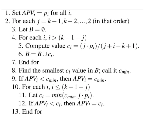
1. Set APVi=pifor all i.
2. For each j=k−1,k−2, ...,2 (in that order) 3. Let B= /0.
4. For each i, i>(k−1−j)
5. Compute value ci= (j·pi)/(j+i−k+1). 6. B=B∪ci.
7. End for
8. Find the smallest civalue in B; call it cmin. 9. If APVi<cmin, then APVi=cmin.
10. For each i, i≤(k−1−j) 11. Let ci=min(cmin,j·pi). 12. If APVi<ci, then APVi=ci. 13. End for
Figure 3: Algorithm for calculating APVs based on Hommel’s procedure
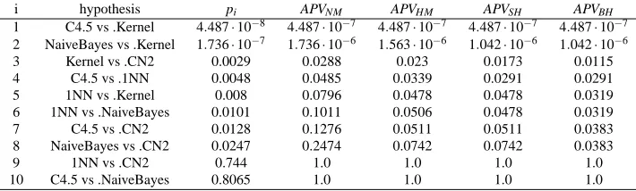
i hypothesis pi APVNM APVHM APVSH APVBH
1 C4.5 vs .Kernel 4.487·10−8 4.487·10−7 4.487·10−7 4.487·10−7 4.487·10−7
2 NaiveBayes vs .Kernel 1.736·10−7 1.736·10−6 1.563·10−6 1.042·10−6 1.042·10−6
3 Kernel vs .CN2 0.0029 0.0288 0.023 0.0173 0.0115 4 C4.5 vs .1NN 0.0048 0.0485 0.0339 0.0291 0.0291 5 1NN vs .Kernel 0.008 0.0796 0.0478 0.0478 0.0319 6 1NN vs .NaiveBayes 0.0101 0.1011 0.0506 0.0478 0.0319 7 C4.5 vs .CN2 0.0128 0.1276 0.0511 0.0511 0.0383 8 NaiveBayes vs .CN2 0.0247 0.2474 0.0742 0.0742 0.0383
9 1NN vs .CN2 0.744 1.0 1.0 1.0 1.0
10 C4.5 vs .NaiveBayes 0.8065 1.0 1.0 1.0 1.0
Table 5: APVs obtained in the example by Nemenyi (NM), Holm (HM), Shaffer’s static (SH) and Bergmann-Hommel’s dynamic (BH)
4. Experimental Framework
In this section, we want to determine the power and behavior of the studied procedures through the experiments in which we repeatedly compared the classifiers on sets of ten randomly chosen data sets, recording the number of equivalence hypothesis rejected and APVs. We follow a similar method used in Demˇsar (2006).
The classifiers used are the same as in the case study of the previous subsection: C4.5 with minimum number of item-sets per leaf equal to 2 and confidence level fitted for optimal accuracy and pruning strategy, naive Bayesian learner with continuous attributes discretized using Fayyad and Irani (1993) discretization, classic 1-Nearest-Neighbor classifier with Euclidean distance, CN2 with Fayyad-Irani’s discretizer, star size = 5 and 95% of examples to cover and Kernel classifier with sigmaKernel=0.01, which is the inverse value of the variance that represents the radius of neighborhood. All classifiers are available in KEEL software (Alcal´a-Fdez et al., 2008).5
For performing this study, we have compiled a sample of fifty data sets from the UCI machine learning repository (Asuncion and Newman, 2007), all of them valid for a classification task.6 We measured the performance of each classifier by means of accuracy in test by using ten-fold cross validation. As Demˇsar did, when comparing two classifiers, samples of ten data sets were randomly selected so that the probability for the data set i being chosen was proportional to 1/(1+e−kdi),
where diis the (positive or negative) difference in the classification accuracies on that data set and k is the bias through which we can regulate the differences between the classifiers. With k=0, the selection is purely random and as k is being higher, the selected data sets are favorable to a particular classifier.
In comparisons of multiple classifiers, samples of data sets have to be selected with the prob-abilities computed from the differences in accuracy of two classifiers. We have chosen C4.5 and 1-NN, due to the fact that we have found significant differences between them in the study con-ducted before (Section 2.2) which involved thirty data sets. Note that the repeated comparisons done here only involve ten data sets each time, so the rejection of equivalence of two classifiers is more difficult at the beginning of the process.
5. It is also available athttp://www.keel.es.
Figure 4 shows the results of this study considering the pairwise comparison between C4.5 and 1-NN. It gives an approximation of the power of the statistical procedures considered in this paper. Figure 4(a) reflects the number of times they rejected the equivalence of C4.5 and 1-NN. Obviously, the Bergmann-Hommel procedure is the most powerful, followed by Shaffer’s static procedure. The graphic also informs us about the use of logically related hypothesis, given that the procedures that use this information have a bias towards the same point and those which do not use this information, tend to a lower point than the first. When the selection of data sets is purely random (k=0), the benefit of using the Bergmann-Hommel procedure is appreciable. Figure 4(b) shows the average APV of the same comparison of classifiers. As we can see, the Nemenyi procedure is too conservative in comparison with the remaining procedures. Again, the benefit of using more sophisticated testing procedures is easily noticeable.
0 100 200 300 400 500 600 700 800 900
0 1 2 3 4 5 6 7 8 9 10 11 12 13 14 15 16 17 18 19 20
k re je c te d h y p o th e s e s
Nemenyi Holm Shaffer Bergmann
(a) Number of hypotheses rejected in pairwise compar-isons 0 0.05 0.1 0.15 0.2 0.25 0.3 0.35
0 1 2 3 4 5 6 7 8 9 10 11 12 13 14 15 16 17 18 19 20
k a v e ra g e p -v a lu e
Nemenyi Holm Shaffer Bergmann
(b) Average APV in pairwise comparisons
Figure 4: C4.5 vs. 1-NN
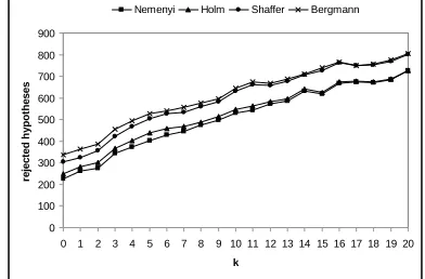
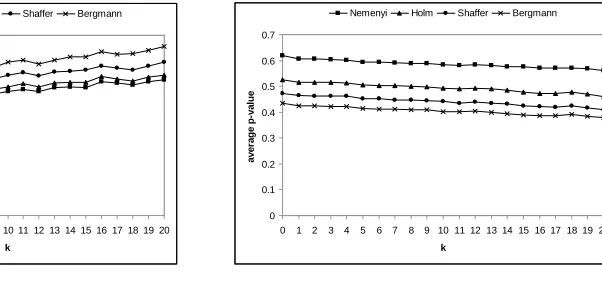
Figure 5 shows the results of this study considering all possible pairwise comparisons in the set of classifiers. It helps us to compare the overall behavior of the four testing procedures. Figure 5(a) presents the number of times they rejected any comparison belonging to the family. Although it could seem that the selection of data sets determined by the difference of accuracy between two classifiers may not influence on the overall comparison, the graphic shows us that it occurs. Further-more, the lines drawn follow a parallel behavior, indicating us the relation and magnitude of power among the four procedures. In Figure 5(b) we illustrate the average APV for all the comparisons of classifiers. We can notice that the conservatism of the Nemenyi test is obvious with respect to the rest of procedures. The benefit of using a more advanced testing procedure is similar with respect to the following less-powerful procedure, except for Holm’s procedure.
Finally, our recommendation on the usage of a certain procedure depends on the results obtained in this paper and in our experience in understanding and implementing them:
• We do not recommend the use of Nemenyi’s test, because it is a very conservative procedure and many of the obvious differences may not be detected.
0 500 1000 1500 2000 2500 3000 3500
0 1 2 3 4 5 6 7 8 9 10 11 12 13 14 15 16 17 18 19 20
k re je c te d h y p o th e s e s
Nemenyi Holm Shaffer Bergmann
(a) Total number of hypotheses rejected
0 0.1 0.2 0.3 0.4 0.5 0.6 0.7
0 1 2 3 4 5 6 7 8 9 10 11 12 13 14 15 16 17 18 19 20
k a v e ra g e p -v a lu e
Nemenyi Holm Shaffer Bergmann
(b) Average APV in all comparisons
Figure 5: All comparisons
• However, conducting the Shaffer static procedure means a not very significant increase of the difficulty with respect to the Holm procedure. Moreover, the benefit of using information about logically related hypothesis is noticeable, thus we strongly encourage the use of this procedure.
• Bergmann-Hommel’s procedure is the best performing one, but it is also the most difficult to understand and computationally expensive. We recommend its usage when the situation requires so (i.e., the differences among the classifiers compared are not very significant), given that the results it obtains are as valid as using other testing procedure.
5. Conclusions
The present paper is an extension of Demˇsar (2006). Demˇsar does not deal in depth with some topics related to multiple comparisons involving all the algorithms and computations of adjusted p-values.
Acknowledgments
This research has been supported by the project TIN2005-08386-C05-01. S. Garc´ıa holds a FPU scholarship from Spanish Ministry of Education and Science. The present paper was submitted as a regular paper in the JMLR journal. After the review process, the action editor Dale Schuurmans encourages us to submit the paper to the special topic on Multiple Simultaneous Hypothesis Testing. We are very grateful to the anonymous reviewers and both action editors who managed this paper for their valuable suggestions and comments to improve its quality.
Appendix A. Source Code of the Procedures
The source code, written in JAVA, that implements all the procedures described in this paper, is available athttp://sci2s.ugr.es/keel/multipleTest.zip. The program allows the input of data in CSV format and obtains as output a LATEX document.
References
J. Alcal´a-Fdez, L. S´anchez, S. Garc´ıa, M.J. del Jesus, S. Ventura, J.M. Garrell, J. Otero, C. Romero, J. Bacardit, V.M. Rivas, J.C. Fern´andez, and F. Herrera. KEEL: A software tool to assess evolu-tionary algorithms to data mining problems. Soft Computing. doi: 10.1007/s00500-008-0323-y, 2008. In press.
A. Asuncion and D.J. Newman. UCI machine learning repository, 2007. URLhttp://www.ics. uci.edu/˜mlearn/MLRepository.html.
R. E. Banfield, L. O. Hall, K. W. Bowyer, and W. P. Kegelmeyer. A comparison of decision tree ensemble creation techniques. IEEE Transactions on Pattern Anaylisis and Machine Intelligence, 29(1):173–180, 2007.
G. Bergmann and G. Hommel. Improvements of general multiple test procedures for redundant systems of hypotheses. In P. Bauer, G. Hommel, and E. Sonnemann, editors, Multiple Hypotheses Testing, pages 100–115. Springer, Berlin, 1988.
P. Clark and T. Niblett. The CN2 induction algorithm. Machine Learning, 3(4):261–283, 1989.
J. Demˇsar. Statistical comparisons of classifiers over multiple data sets. Journal of Machine Learn-ing Research, 7:1–30, 2006.
S. Esmeir and S. Markovitch. Anytime learning of decision trees. Journal of Machine Learning Research, 8:891–933, 2007.
U. M. Fayyad and K. B. Irani. Multi-interval discretization of continuous valued attributes for classification learning. In Proceedings of the 13th International Joint Conference on Artificial Intelligence, pages 1022–1029. Morgan-Kaufmann, 1993.
N. Garc´ıa-Pedrajas and C. Fyfe. Immune network based ensembles. Neurocomputing, 70(7-9): 1155–1166, 2007.
Y. Hochberg. A sharper bonferroni procedure for multiple tests of significance. Biometrika, 75: 800–802, 1988.
Y. Hochberg and D. Rom. Extensions of multiple testing procedures based on Simes’ test. Journal of Statistical Planning and Inference, 48:141–152, 1995.
S. Holm. A simple sequentially rejective multiple test procedure. Scandinavian Journal of Statistics, 6:65–70, 1979.
G. Hommel. A stagewise rejective multiple test procedure. Biometrika, 75:383–386, 1988.
G. Hommel and G. Bernhard. A rapid algorithm and a computer program for multiple test proce-dures using proceproce-dures using logical structures of hypotheses. Computer Methods and Programs in Biomedicine, 43:213–216, 1994.
G. Hommel and G. Bernhard. Bonferroni procedures for logically related hypotheses. Journal of Statistical Planning and Inference, 82:119–128, 1999.
R. L. Iman and J. M. Davenport. Approximations of the critical region of the friedman statistic. Communications in Statistics, pages 571–595, 1980.
C. Marrocco, R. P. W. Duin, and F. Tortorella. Maximizing the area under the ROC curve by pairwise feature combination. Pattern Recognition, 41:1961–1974, 2008.
G. J. McLachlan. Discriminant Analysis and Statistical Pattern Recognition. Wiley Series in Prob-ability and Mathematical Statistics, 2004.
J. F. Murray, G. F. Hughes, and K. Kreutz-Delgado. Machine learning methods for predicting failures in hard drives: A multiple-instance application. Journal of Machine Learning Research, 6:783–816, 2005.
P. B. Nemenyi. Distribution-free Multiple Comparisons. PhD thesis, Princeton University, 1963.
M. N´u˜nez, R. Fidalgo, and R. Morales. Learning in environments with unknown dynamics: Towards more robust concept learners. Journal of Machine Learning Research, 8:2595–2628, 2007.
A. B. Owen. Infinitely imbalanced logistic regression. Journal of Machine Learning Research, 8: 761–773, 2007.
J. R. Quinlan. Programs for Machine Learning. Morgan Kauffman, 1993.
D. M. Rom. A sequentially rejective test procedure based on a modified bonferroni inequality. Biometrika, 77:663–665, 1990.
J.P. Shaffer. Modified sequentially rejective multiple test procedures. Journal of the American Statistical Association, 81(395):826–831, 1986.
D. Sheskin. Handbook of Parametric and Nonparametric Statistical Procedures. Chapman & Hall/CRC, 2003.
R.J. Simes. An improved Bonferroni procedure for multiple tests of significance. Biometrika, 73: 751–754, 1986.
P. H. Westfall and S. S. Young. Resampling-Based Multiple Testing: Examples and Methods for p-value Adjustment. John Wiley and Sons, 2004.
S. P. Wright. Adjusted p-values for simultaneous inference. Biometrics, 48:1005–1013, 1992.
Y. Yang, G. Webb, K. Korb, and K. M. Ting. Classifying under computational resource constraints: anytime classification using probabilistic estimators. Machine Learning, 69:35–53, 2007a.
Y. Yang, G. I. Webb, J. Cerquides, K. B. Korb, J. Boughton, and K. M. Ting. To select or to weigh: A comparative study of linear combination schemes for superparent-one-dependence estimators. IEEE Transcations on Knowledge and Data Engineering, 19(12):1652–1665, 2007b.