On the Consistency of Feature Selection
using Greedy Least Squares Regression
Tong Zhang∗ [email protected]
Statistics Department 110 Frelinghuysen Road Rutgers University, NJ 08854
Editor: Bin Yu
Abstract
This paper studies the feature selection problem using a greedy least squares regression algorithm. We show that under a certain irrepresentable condition on the design matrix (but independent of the sparse target), the greedy algorithm can select features consistently when the sample size ap-proaches infinity. The condition is identical to a corresponding condition for Lasso.
Moreover, under a sparse eigenvalue condition, the greedy algorithm can reliably identify fea-tures as long as each nonzero coefficient is larger than a constant times the noise level. In compar-ison, Lasso may require the coefficients to be larger than O(√s)times the noise level in the worst case, where s is the number of nonzero coefficients.
Keywords: greedy algorithm, feature selection, sparsity
1. Introduction
We are interested in the statistical feature selection problem for least squares regression. Let X= [x1, . . . ,xd]∈Rn×dbe an n×d data matrix with xj∈Rn( j=1, . . . ,d) as its columns. Assume that
the response vector y= [y1, . . . ,yn]∈Rnis generated from a sparse linear combination of the basis
vectors{xj}plus a zero-mean stochastic noise vector z∈Rn:
y=X ¯β+z=
d
∑
j=1
¯
βjxj+z, (1)
where most coefficients ¯βj equal zero. The goal of feature selection is to identify the set of
non-zeros{j : ¯βj6=0}, where ¯β= [β¯1, . . . ,β¯d]. The purpose of this paper is study the performance of
greedy least squares regression for feature selection.
The following notations are used throughout the paper. Givenβ∈Rd, define
supp(β) ={j :βj6=0}.
Given x∈Rnand ¯F⊂ {1, . . . ,d}, let
ˆ
βX(F¯,x) =min
β∈Rd
1
nkXβ−xk
2
2 subject to supp(β)⊂F¯.
That is, ˆβX(F¯,x)is the least squares solution with coefficients restricted to ¯F.
Given ¯F∈ {1, . . . ,d}, we let XF¯ be the n× |F¯|matrix that is the restriction of columns of X to
¯
F. That is, XF¯’s columns are the basis functions xj with j∈F arranged in the ascending order. The¯
following quantity, appeared in Tropp (2004), is important in our analysis (also see Wainwright, 2006):
µX(F¯) =max j∈/F¯ k(X
T
¯
FXF¯)−1XFT¯xjk1.
We also define for all ¯F⊂ {1, . . . ,d}
ρX(F¯) =inf
1 nkXβk
2
2/kβk22: supp(β)⊂F¯
.
This quantity is the smallest eigenvalue of the restricted design matrix 1nXFT¯XF¯, which has also
appeared in previous work such as Wainwright (2006) and Zhao and Yu (2006). The requirement thatρX(F) is bounded away from zero for small|F|is often referred to as the sparse eigenvalue
condition (or the restricted isometry condition).
2. Related Work
The feature selection problem of estimating supp(β¯)from observation y defined in (1) has attracted significant attention in recent years. One of the frequently used method for feature selection is Lasso, which solves the following L1regularization problem:
ˆ
β=arg min
β
1 n
d
∑
j=1
βjxj−y
2 2
+λkβk1
, (2)
whereλ>0 is an appropriately chosen regularization parameter.
The effectiveness of feature selection using Lasso was established in Zhao and Yu (2006) (also see Meinshausen and Buhlmann, 2006) under irrepresentable conditions that depend on the signs of the true target sgn(β¯). Results established in this paper have cruder forms that depend only on the design matrix but not the sparse target ¯β. Such conditions have also been studied by Zhao and Yu (2006) (also see Wainwright, 2006).
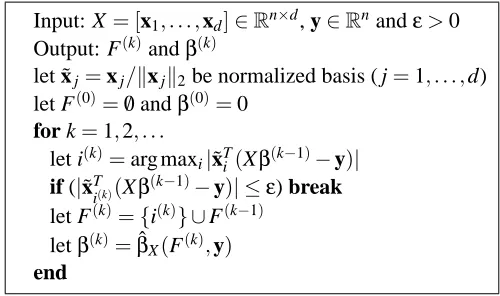
In addition to Lasso, greedy algorithms have also been widely used for feature selection. Greedy algorithms for least squares regression are called matching pursuit in the signal processing commu-nity (Mallat and Zhang, 1993). The particular algorithm analyzed in this paper (some time referred to as orthogonal matching pursuit or OMP) is presented in Figure 1. The algorithm is often called forward greedy selection in the machine learning literature.
This paper investigates the behavior of greedy least squares algorithm in Figure 1 for feature selection under the stochastic noise model (1). Our result extends that of Tropp (2004), which only considered the situation without stochastic noise. It was shown by Tropp (2004) that µX(F¯)<1 is
sufficient for the greedy algorithm to identify the correct feature set supp(β¯)when the noise vector
z=0. The main contribution of this paper is to generalize Tropp’s analysis to handle non-zero sub-Gaussian stochastic noise vectors. In particular, we will establish conditions on minj∈supp(β¯)|β¯j|and
Input: X= [x1, . . . ,xd]∈Rn×d, y∈Rnandε>0
Output: F(k)andβ(k)
let ˜xj=xj/kxjk2be normalized basis ( j=1, . . . ,d)
let F(0)=/0andβ(0)=0
for k=1,2, . . .
let i(k)=arg maxi|˜xTi (Xβ(k−1)−y)|
if (|˜xTi(k)(Xβ(k−1)−y)| ≤ε) break let F(k)={i(k)} ∪F(k−1)
letβ(k)=βˆX(F(k),y)
end
Figure 1: Greedy Least Squares Regression (OMP)
regularization conditionλ in the Lasso formulation (2), which is necessary both in theory and in practice. The condition on minj∈supp(β¯)|β¯j|also naturally appears in the analysis of Lasso (Zhao
and Yu, 2006). In fact, our result shows that the condition of minj∈supp(β¯)|β¯j|required for greedy
algorithm is weaker than the corresponding condition for Lasso.
The greedy algorithm analysis employed in this paper is a combination of an observation by Tropp (2004, see Lemma 11) and some technical lemmas for the behavior of greedy least squares regression by Zhang (2008), which are included in Appendix A for completeness. Note that Zhang (2008) only studied a forward-backward procedure, but not the more standard forward greedy algo-rithm considered here. In this paper, both the employment of the condition µX(F¯)<1 and the proof
in Appendix B are new.
As we shall see in this paper, the condition µX(F¯)≤1 is necessary for the success of the forward
greedy procedure. It is worth mentioning that Lasso is consistent in parameter estimation under a weaker sparse eigenvalue condition, even if the condition µX(F¯)≤1 fails (which means Lasso may
not estimate the true feature set correctly): for example, see Meinshausen and Yu (2008) and Zhang (2009). Although similar results may be obtained for greedy least squares regression, when the condition µX(F¯)≤1 fails, it was shown by Zhang (2008) that the performance of greedy algorithm
can be improved by incorporating backward steps. In contrast, results in this paper show that if the design matrix satisfies the additional condition µX(F¯)<1, then the standard forward greedy
algorithm will be successful without complicated backward steps.
3. Feature Selection using Greedy Least Squares Regression
We would like to establish conditions under which the forward greedy algorithm in Figure 1 never makes any mistake (with large probability), and thus suitable for feature selection. For convenience, we state an assumption before stating the theoretical result.
Assumption 1 Assume that
• The basis functions are normalized such that 1nkxjk22=1 for all j=1, . . . ,d.
• The target function is truly sparse: there exists ¯β∈Rdwith ¯F=supp(β¯)such that Ey=X ¯β.
• y= [yi]i=1,...,n are independent (but not necessarily identically distributed) sub-Gaussians:
there existsσ≥0 such that∀i∈ {1, . . . ,n}and∀t∈R, Eyie
t(yi−Eyi)≤eσ2t2/2.
Both Gaussian and bounded random variables are sub-Gaussian using the above definition. For example, if a random variable ξ∈[a,b], then Eξet(ξ−Eξ) ≤e(b−a)2t2/8. If a random variable is Gaussian:ξ∼N(0,σ2), then E
ξetξ≤eσ2t2/2.
The following theorem gives conditions under which the forward greedy algorithm can identify the correct set of features.
Theorem 1 Consider the greedy least squares algorithm in Figure 1, where Assumption 1 holds.
Given anyη∈(0,0.5), with probability larger than 1−2η, if the stopping criterion satisfies
ε> 1
1−µX(F¯)
σp
2 ln(2d/η), min
j∈F¯|
¯
βj| ≥3ερX(F¯)−1/√n,
then when the procedure stops, we have F(k−1)=F and¯
kβ(k−1)−β¯k
∞≤σ
q
(2 ln(2|F¯|/η))/(nρX(F¯)).
The result is a simple consequence of the following slightly more general theorem (its proof is left to Appendix B).
Theorem 2 Consider the greedy least squares algorithm in Figure 1, where Assumption 1 holds.
Given anyη∈(0,0.5), with probability larger than 1−2η, if the stopping criterion satisfies
ε> 1
1−µX(F¯)
σp
2 ln(2d/η),
then when the procedure stops, the following claims are true:
• F(k−1)⊂F.¯
• |F¯−F(k−1)| ≤2|{j∈F :¯ |β¯j|<3ερX(F¯)−1/√n}| • kβ(k−1)−βˆ
X(F¯,y)k2≤ερ(F¯)−1
p
|F¯−F(k−1)|/n. • kβˆX(F¯,y)−β¯k∞≤σ
p
(2 ln(2|F¯|/η))/(nρX(F¯)).
In the following, we discuss some consequences of Theorem 1 and Theorem 2, and compare them with those of Lasso. Let k(ε)be the number of j∈F such that¯ |β¯j|<3ερX(F¯)−1/√n.
The-orem 2 implies that|F¯−F(k−1)| ≤2k(ε); that is,|F¯−F(k−1)|is small when k(ε)is small. In such case, the feature set F(k−1)selected by the greedy least squares algorithm is approximately correct. Moreover, we haveβ(k−1)≈β¯. In fact, one can show (e.g., see Zhang, 2008) that with probability larger than 1−η:
kβˆX(F¯,y)−β¯k2≤σ
q
|F¯|/(ρ(F¯)n)[1+p
20 ln(1/η)].
By combining this estimate with Theorem 2, we have
kβ(k−1)−β¯k2≤σ
q
That is, kβ(k−1)−β¯k2 =O(p
|F¯|/n+εp
k(ε)/n). This implies that when µX(F¯) <1, greedy
least squares regression leads to a good estimation of the true parameter ¯β. By choosing ε=
O(σp
ln(2d/η)), we obtain kβ(k−1)−β¯k2=O(
p
|F¯|/n+p
k(ε)ln d/n). The corresponding re-sult for the Lasso estimator ˆβ in (2) iskβˆ−β¯k2=O(λ
p
|F¯|/n), where we require λto be of the orderσpln(d/η)/n or larger. Therefore, if k(ε)is small, then Lasso is inferior due to the extra ln d factor. This factor is inherent to the L1regularization in Lasso, which introduces a bias that cannot
be removed.
In this paper, we are mainly interested in the situation k(ε) =0, which implies that with the stopping criterion ε, greedy least squares regression can correctly identify all features with large probability. Note that in order to correctly identify all features (F(k−1) =F), the requirement¯ minj∈F¯|β¯j| ≥ 3ερX(F¯)−1/√n in Theorem 1 is natural. Observe that we may take
ε=σp3 ln(d/η)/(1−µX(F¯)). This means that under the assumption of Theorem 1, it is
pos-sible to identify all features correctly using the greedy least squares algorithm as long as the target coefficients ¯βj( j∈F) are larger than the order¯ σ
p
ln(d/η)/n.
In fact, sinceσpln(d/η)/n is the noise level, if there exists a target coefficient ¯βjthat is smaller
than O(σp
ln(d/η)/n)in absolute value, then we cannot distinguish such a small coefficient from zero (or noise) with large probability. Therefore when the condition µX(F¯)<1 holds, it is not
possible to do much better than greedy least squares regression except for the constant hidden in O(·)and its dependency onρ(F¯)and µX(F¯).
In comparison, for Lasso, the condition required of minj∈F¯|β¯j|depends not only onρ(F¯)−1and
(1−µX(F¯))−1, but also on the quantityk(XFT¯XF¯)−1k∞,∞(see Wainwright, 2006), where
k(XFT¯XF¯)−1k∞,∞= sup
u∈R|F¯|
k(XFT¯XF¯)−1uk∞ kuk∞ .
Consider the matrix(XFT¯XF¯)−1=I+0.5B/
p
|F¯|, where Bi,j=1 when either i=1 or j=1 or i=j, and Bi,j=0 otherwise. Then it is not hard to verify thatρ(F¯)−1<2 andk(XFT¯XF¯)−1k∞,∞>0.5
p
|F¯| (by taking u= [1, . . . ,1]). This means that in the worst case, we can find matrix XFT¯XF¯ such that
k(XFT¯XF¯)−1k∞,∞>0.25
q
|F¯|ρ(F¯)−1.
Therefore, if we only assume that ρ(F¯) is bounded away from zero without using the quantity
k(XFT¯XF¯)−1k∞,∞, the feature consistency result in Zhao and Yu (2006) and Wainwright (2006) for Lasso requires the condition
min
j∈supp(β¯)| ¯
βj| ≥cσ
q
|F¯|ln(d/η)/n
for some constant c that is proportional toρ(F¯)−1(1−µ
X(F¯))−1. This is a more restrictive condition
than that of greedy least squares regression. Unfortunately, the factorp|F¯|cannot be removed for Lasso, unless we make the additional and stronger assumption thatk(XFT¯XF¯)−1k∞,∞=O(ρ(F¯)−1).
As we discussed after Theorem 2, the bias of L1-regularization also leads to suboptimal
estima-tion for Lasso. For example, for the greedy algorithm, we can showkβˆX(F¯,y)−β¯k2=O(σ
p
|F¯|/n) and kβˆX(F¯,y)−β¯k∞=O(σ
p
ln|F¯|/n). Under the conditions of Theorem 1, we have β(k−1)=
ˆ
βX(F¯,y), and thus kβ(k−1)−β¯k2 =O(σ
p
|F¯|/n) and kβ(k−1)−β¯k∞=O(σp
the same conditions, for the Lasso estimator ˆβ of (2), we havekβˆ−β¯k2=O(σ
p
|F¯|ln d/n)and
kβˆ−β¯k∞=O(σp
ln d/n). The ln d factor (bias) is inherent to Lasso, which can be removed with two-stage procedures (e.g., Zhang, 2009). However, such procedures are less robust and more com-plicated than the simple greedy algorithm.
4. Feature Selection Consistency
As we have mentioned before, the effectiveness of feature selection using Lasso was established by Zhao and Yu (2006), under more refined irrepresentable conditions that depend on the signs of the true target sgn(β¯). In comparison, the condition µX(F¯)<1 in Theorem 2 depends only on the design
matrix but not the sparse target ¯β. That is, the condition is with respect to the worst case choice of ¯
β with support supp(β¯) =F. Due to the complexity of greedy procedure, we cannot establish a¯ simple target dependent condition that ensures feature selection consistency. This means for any specific target, the behavior of forward greedy algorithm and Lasso might be different, and one may be preferred over the other under different scenarios. Experiments in Zhang (2008) illustrated this point.
In the following, we introduce the target independent irrepresentable conditions that are equiv-alent to the irrepresentable conditions of Zhao and Yu (2006) with the worst case choice of sgn(β¯)
(also see Wainwright, 2006).
Definition 3 Consider a sequence of problems indexed by n: at each sample size n, let X(n)be an n×d(n)dimensional data matrix, and we observe y(n)∈Rn that is corrupted with noise. Let ¯F(n) be the feature set, where Ey(n)=X(n)β¯(n)and supp(β¯(n)) =F¯(n).
We say that the sequence satisfies the strong target independent irrepresentable condition if there existsδ>0 such that limn→∞µX(n)(F¯(n))≤1−δ.
We say that the sequence satisfies the weak target independent irrepresentable condition if µX(n)(F¯(n))≤1 for all sufficiently large n.
It was shown by Zhao and Yu (2006) that the strong (target independent) irrepresentable condition is sufficient for Lasso to select features consistently for all possible sign combination of ¯β(n)when n→∞(under appropriate assumptions). In addition, the weak (target independent) irrepresentable condition is necessary for Lasso to select features consistently when n→∞. The target independent irrepresentable conditions are considered by Zhao and Yu (2006) and Wainwright (2006). Similar conditions were also considered by Tropp (2004) without stochastic noise.
Results parallel to that of Lasso can be obtained for Algorithm 1. Specifically, the following two theorems show that the strong target independent irrepresentable condition is sufficient for Algo-rithm 1 to select features consistently, while the weak target independent irrepresentable condition is necessary.
Theorem 4 Consider regression problems indexed by the sample size n, and use notations in
Defini-tion 3. Let AssumpDefini-tion 1 hold, with noiseσindependent of n. Assume that the strong irrepresentable condition holds. For each problem of sample size n, denote by Fnthe feature set from Algorithm 1
when it stops withε=ns/2for some s∈(0,1]. Then for all sufficiently large n, we have P(Fn6=F¯(n))≤exp(−ns/ln n)
1. dn≤exp(ns/ln n)
2. minj∈F¯(n)|β¯(jn)| ≥3n(s−1)/2/ρ(F¯(n)).
Proof When n is sufficiently large, the two conditions of Theorem 1 hold withη=0.5 exp(−ns/ln n). Therefore the theorem is a direct consequence.
Theorem 5 Consider regression problems indexed by the sample size n, and use notations in
Defini-tion 3. Let AssumpDefini-tion 1 hold, with noiseσindependent of n. Assume that the weak irrepresentable condition is violated at sample sizes n1<n2<···. There exist targets ¯β(nj)with arbitrarily large
mini
∈F¯(n j)|β¯i(nj)|, such that at each sample size nj, Algorithm 1 chooses a basis i(1)∈/F in the first¯
step with probability larger than 0.5.
Proof By definition of µX(F¯), there exists v= (XFT¯XF¯)u∈R|
¯
F|such that
µX(F¯) =max j∈/F¯ k(X
T
¯
FXF¯)−1XFT¯xjk1 =max
j∈/F¯
|vT(XFT¯XF¯)−1XFT¯xj|
kvk∞
=max
j∈/F¯
|uTXFT¯xj|
k(XFT¯XF¯)uk∞ = maxj∈/F|x
T jXF¯u|
maxi∈F¯|(xTi XF¯)u|
.
Therefore if µX(F¯)>1, we can find u∈R|F¯|such that maxj∈/F|xTjXF¯u|>maxi∈F¯|(xTi XF¯)u|.
Consider an arbitrary sequence δn >0 (n =1,2, . . .). At any sample size n =nj, since
µX(n)(F¯(n))>1, we can find a sufficiently large target vector ¯β(n)such that
max
i∈F¯(n)|x
T
i X(n)β¯(n)|< max j∈/F¯(n)|x
T
jX(n)β¯(n)| −2δn. (3)
Now we may takeδn=σ
p
2n ln(4dn); then Lemma 8 implies that with probability larger than 0.5,
maxj∈{1,...,d}|xTj(y−X(n)β¯(n))| ≤δn. Therefore (3) implies that
max
i∈F¯(n)[|x
T
i X(n)β¯(n)|+|xTi (y−X(n)β¯(n))|]< max j∈/F¯(n)[|x
T
jX(n)β¯(n)| − |xTj(y−X(n)β¯(n))|].
Therefore
max
i∈F¯(n)|x
T
i y|< max j∈/F¯(n)|x
T jy|.
5. Conclusion
We have shown that weak and strong target independent irrepresentable conditions are necessary and sufficient conditions for a greedy least squares regression algorithm to select features consistently. These conditions match the target independent versions of the necessary and sufficient conditions for Lasso by Zhao and Yu (2006).
Moreover, if the eigenvalue ρ(F¯) is bounded away from zero, then the greedy algorithm can reliably identify features as long as each nonzero coefficient is larger than a constant times the noise level. In comparison, under the same condition, Lasso may require the coefficients to be larger than O(√s)times the noise level, where s is the number of nonzero coefficients. This implies that under some conditions, greedy least squares regression may potentially select features more effectively than Lasso in the presence of stochastic noise.
Although the target independent versions of the irrepresentable conditions for greedy least squares regression match those of Lasso, our result does not show which algorithm is better for any specific target. In fact, the target specific behaviors of the two algorithms are different, and one may be preferred over the other under different scenarios.
Acknowledgments
This paper is the outcome of some private discussion with Joel Tropp, which drew the author’s attention to the similarities and differences between orthogonal matching pursuit and Lasso for estimating sparse signals.
Appendix A. Auxiliary Lemmas
The following technical lemmas from Zhang (2008) are needed to analyze the behavior of greedy least squares regression under stochastic noise. For completeness, we include them here with proofs. The following lemma relates the squared error reduction in one greedy step to correlation coef-ficients.
Lemma 6 For all x,x′,y∈Rn, we have
inf
α∈Rkx+αx
′−yk2
2=kx−yk22−((x−y)Tx′)2/kx′k22.
Proof The equality follows from simple algebra with the optimalαachieved at−(x−y)Tx′/kx′k2 2.
The following lemma provides a bound on the squared error reduction of one forward greedy step. Some ingredients of the proof has appeared in Natarajan (1995).
Lemma 7 Let Assumption 1 hold. Consider F⊂F¯ ⊂ {1, . . . ,d}. Letβ′=βˆX(F¯,y),β=βˆX(F,y),
x′=Xβ′, and x=Xβ. Then
inf
α∈R,j∈F¯−Fkx+αxj−yk
2
2≤ kx−yk22− ρ(F¯)
|F¯−F|kx−x′k
Proof For all j∈F, we havekx+αxj−yk22 achieves the minimum atα=0. This implies that (x−y)Tx
j=0 for j∈F. Therefore we have
(x−y)T
∑
j∈F¯−F(β′j−βj)xj
=(x−y)T
∑
j∈F¯∪F(β′j−βj)xj= (x−y)T(x′−x)
=− kx−x′k2
2+ (x′−y)T(x′−x) =−kx−x′k22.
The last quality follows from the definition ofβ′=βˆX(F¯,y)and F⊂F, which implies that¯ (x′−
y)T(x′−x) =0. Now, let s′=|F¯−F|, then the above inequality leads to the following derivation
∀η>0:
s′ inf
j∈F¯−Fkx+η(β
′
j−βj)xj−yk22
≤
∑
j∈F¯−F
kx+η(β′j−βj)xj−yk22 =s′kx−yk2
2+η2
∑
j∈F¯−F
(β′j−βj)2kxjk22+2η(x−y)T
∑
j∈F¯−F
(β′j−βj)xj
=s′kx−yk22+nη2
∑
j∈F¯−F
(β′j−βj)2−2ηkx′−xk22.
Note that in the last equation, we have usedkxjk22=n in Assumption 1. By optimizing overη, we
obtain
s′ inf
j∈F¯−Fkx
+η(β′j−βj)xj−yk22
≤s′kx−yk22− kx ′−xk4
2
n∑j∈F¯(β′j−βj)2 ≤
s′kx−yk22−ρ(F¯)kx′−xk2 2.
This leads to the lemma.
The following lemma is a standard empirical processes bound for sub-Gaussian random vari-ables. The bound is used to derive probability estimates in our analysis.
Lemma 8 Consider n independent random variables ξ1, . . . ,ξn such that Eet(ξi−Eξi)≤eσ
2
it2/2 for
all t and i. Consider gi,jfor i=1, . . . ,n and j=1, . . . ,m, we have for allη∈(0,1), with probability
larger than 1−η:
sup
j | n
∑
i=1
gi,j(ξi−Eξi)| ≤a
p
2 ln(2m/η),
where a2=sup
j∑ni=1g2i,jσ2i.
Proof For a fixed j, we let sj=∑ni=1gi,j(ξi−Eξi); then by assumption, E(etsj+e−tsj)≤2ea
2t2/2 , which implies that for allε>0: P(|sj| ≥ε)etε≤2ea
2t2/2
. Now let t=ε/a2, we obtain:
P
n
∑
i=1
gi,j(ξi−Eξi)
≥ε
!
This implies that
P
"
sup
j
n
∑
i=1
gi,j(ξi−Eξi)
≥ε
#
≤m sup
j
P
"
n
∑
i=1
gi,j(ξi−Eξi)
≥ε
#
≤2me−ε2/(2a2).
This implies the lemma.
The following lemma gives a bound on the infinity norm of the difference between the estimated parameter ˆβX(F¯,y)and the true parameter ¯βwhen the set of features ¯F are known in advance.
Lemma 9 Let Assumption 1 hold. Consider any fixed ¯F ⊂ {1, . . . ,d}. For all η∈(0,1), with probability larger than 1−η, we have
kβˆX(F¯,y)−βˆX(F¯,Ey)k∞≤σ
q
(2 ln(2|F¯|/η))/(nρ(F¯)).
Proof For simplicity, let G=XF¯ and ¯k =|F¯|. Let ˆβ′ ∈R¯k and ¯β′ ∈R¯k be the restrictions of
ˆ
βX(F¯,y)∈Rd and ˆβX(F¯,Ey)∈Rd to ¯F respectively. Algebraically, we have ˆβ′ = (GTG)−1GTy
and ¯β′= (GTG)−1GTEy. It follows that
ˆ
β′−β¯′= (GTG)−1GT(y
−Ey).
Therefore
|βˆ′j−β¯′j|=|eTj(GTG)−1GT(y−Ey)|.
Lemma 8 implies that with probability larger than 1−η, for all j:
|eTj(GTG)−1GT(y−Ey)| ≤σkeTj(GTG)−1GTk2
q
2 ln(2¯k/η).
Since by definition,ρ(F¯)n is no larger than the smallest eigenvalue of GTG, the desired inequality
follows from the estimate
keTj(GTG)−1GTk2
2=eTj(GTG)−1ej≤1/(nρ(F¯)).
The following lemma estimates the correlation coefficient of xj with j∈/F.¯
Lemma 10 Let Assumption 1 hold. Assume also that Ey=X ¯βwith supp(β¯)⊂F¯ ⊂ {1, . . . ,d}. For allη∈(0,1), with probability larger than 1−η, we have
max
j∈/F¯ |
(X ˆβX(F¯,y)−y)Txj| ≤σ
p
2n ln(2d/η).
Proof Let P be the projection operator to the subspace spanned by{xj : j∈F¯}onRn. Lemma 8
implies that with probability larger than 1−η:
sup
j=1,...,d|
(y−Ey)T(I−P)xj| ≤σ
p
where we have usedkxjk2=√n. Let ˆx=X ˆβX(F¯,y). Since(ˆx−y)Txj=0 for all j∈F, we have¯
ˆx=Py. Moreover, since(I−P)Ey= (I−P)X ¯β=0, we have
(y−Ey)T(I−P)x
j= ((I−P)y−(I−P)Ey)Txj= (y−ˆx)Txj.
Combine this equation with the previous inequality, we obtain the desired bound.
Appendix B. Proof of Theorem 2
Before the formal proof, we give a brief outline of the main argument. First, Lemma 10 im-plies that with large probability, maxj∈/F¯|(X ˆβX(F¯,y)−y)Txj|is small. Using this fact, and the
assumption that µX(F¯)<1, it follows from Lemma 11 below that when supp(β(k−1)) ⊂F, ei-¯
ther maxi|(Xβ(k−1)−y)Txi| is sufficiently small (which implies that the greedy procedure stops
andβ(k−1)≈β¯), or maxj∈/F¯|(Xβ(k−1)−y)Txj|<maxi∈F¯|(Xβ(k−1)−y)Txi|(which implies that the
greedy procedure chooses a direction i(k)∈F in the next iteration). The claims of the theorem then¯ follow by induction.
We start the formal proof by introducing the following critical lemma, which generalizes the essential idea of Tropp (2004). Note that the result there only considered the case X ˆβX(F¯,y) =y.
Lemma 11 Considerβ∈Rd such that supp(β)⊂F. We have¯
max
j∈/F¯ |(Xβ−y)
Tx
j| ≤max j6∈F¯ |(X ˆβX(
¯
F,y)−y)Txj|+µX(F¯)max
i∈F¯ |(Xβ−y)
Tx i|.
Proof Letβ′=βˆX(F¯,y). Note that(Xβ′−y)Txi=0 when i∈F. Therefore¯
max
i∈F¯ |(Xβ−y)
Tx
i|=max i∈F¯ |x
T
i X(β−β′)|=kXFT¯XF¯(β−β′)k∞.
Let v=XFT¯XF¯(β−β′), then the definition of µX(F¯)implies that
µX(F¯)≥max j∈/F¯
|xTjXF¯(XFT¯XF¯)−1v|
kvk∞ =
maxj∈/F¯|xTjXF¯(β−β′)|
kXT
¯
FXF¯(β−β′)k∞
.
We obtain from the above
max
j∈/F¯ |x
T
jX(β−β′)| ≤µX(F¯)kXFT¯XF¯(β−β′)k∞=µX(F¯)max
i∈F¯ |(Xβ−y)
Tx i|.
Now, the lemma follows from the simple inequality
max
j∈/F¯ |(Xβ−y)
Tx
j| ≤max j∈/F¯ |x
T
jX(β−β′)|+max j∈/F¯ |x
T
j(Xβ′−y)|
Now we are ready to prove the theorem. From Lemma 9, we obtain with probability larger than 1−η,
kβˆX(F¯,y)−β¯k∞≤σ
q
From Lemma 10, we obtain with probability larger than 1−η,
max
j∈/F¯ |
(X(βˆX(F¯,y))−y)T˜xj| ≤σ
p
2 ln(2d/η)<(1−µX(F¯))ε. (4)
With probability larger than 1−2η, both claims hold.
We now proceed by induction on k to show that F(k−1)⊂F before the procedure stops. Assume¯ the claim is true after k−1 steps for k≥1. By induction hypothesis, we have F(k−1)⊂F at the¯ beginning of step k. Therefore Lemma 7 implies
min
α,i∈F¯kXβ
(k−1)+αx
i−yk22≤ kXβ(k−1)−yk22−
ρ(F¯)
|F¯−F(k−1)|kX(β
(k−1)−βˆ
X(F¯,y))k22.
Using the above inequality, we obtain from Lemma 6 the following bound on the correlation coef-ficients:
max
i∈F¯ |(Xβ
(k−1)
−y)T˜xi|=
kXβ(k−1)−yk22−min
α,i∈F¯kXβ
(k−1)+αx
i−yk22
1/2
≥
p
ρ(F¯)
p
|F¯−F(k−1)|kX(β (k−1)
−βˆX(F¯,y))k2
≥ √
nρ(F¯)
p
|F¯−F(k−1)|kβ
(k−1)−βˆ
X(F¯,y)k2.
We only need to consider the following two scenarios:
• kβ(k−1)−βˆ
X(F¯,y)k2>ερ(F¯)−1
p
|F¯−F(k−1)|/n. In this case, we have
max
i∈F¯ |
(Xβ(k−1)−y)T˜x
i|>ε>max j∈/F¯ |
(X ˆβX(F¯,y)−y)T˜xj|/(1−µX(F¯)).
The second inequality is due to (4). Now by combining this estimate with Lemma 11, we obtain
max
j∈/F¯ |(Xβ
(k−1)−y)T˜x
j|<max i∈F¯ |(Xβ
(k−1)−y)T˜x i|.
This implies that i(k)∈F and the procedure does not stop.¯
• kβ(k−1)−βˆX(F¯,y)k2≤ερ(F¯)−1p
|F¯−F(k−1)|/n. In this case, we have the following scenarios:
1. i(k)∈/F: By Lemma 11, we must have:¯
max
i∈F¯ |(Xβ−y)
T˜x
i| ≤max
j∈/F¯ |(Xβ−y)
T˜x j|
≤max
j6∈F¯ |(X ˆβX(
¯
F,y)−y)T˜xj|+µX(F¯)max
i∈F¯ |(Xβ−y)
T˜x i|
≤max
j6∈F¯ |
(X ˆβX(F¯,y)−y)T˜xj|+µX(F¯)max j∈/F¯ |
Therefore
max
j∈/F¯ |(Xβ−y)
T˜x j| ≤
1 1−µX(F¯)
max
j6∈F¯ |(X ˆβX(
¯
F,y)−y)T˜xj|<ε.
The last inequality is due to (4). This implies that the procedure stops.
2. i(k)∈F and the procedure does not stop.¯ 3. i(k)∈F and the procedure stops.¯
The above situations imply that if the procedure does not stop, then i(k)∈F. If the procedure¯ stops, then
kβ(k−1)−βˆX(F¯,y)k2≤ερ(F¯)−1
q
|F¯−F(k−1)|/n.
Therefore by induction, when the procedure stops, the following three claims hold:
• F(k−1)⊂F.¯
• kβ(k−1)−βˆ
X(F¯,y)k2≤ερX(F¯)−1
p
|F¯−F(k−1)|/n. • kβˆX(F¯,y)−β¯k∞≤σ
p
(2 ln(2|F¯|/η))/(nρX(F¯))<ε/
p
nρX(F¯).
Now, we can letγ=√8ερX(F¯)−1/√n, then the above claims imply that
γq|{j∈F¯−F(k−1):|β¯
j| ≥γ}|
≤
∑
j∈F¯−F(k−1)
|β¯j|2
1/2
≤
∑
j∈F¯−F(k−1)
|β¯j−βˆX(F¯,y)|2
1/2 +
∑
j∈F¯−F(k−1)
|βˆX(F¯,y)|2
1/2
≤
q
|F¯−F(k−1)|kβ¯−βˆX(F¯,y)k∞+kβ(k−1)−βˆ
X(F¯,y)k2 <
q
|F¯−F(k−1)|/(nρ
X(F¯))ε+ερX(F¯)−1
q
|F¯−F(k−1)|/n ≤2ερX(F¯)−1
q
|F¯−F(k−1)|/n=γq|F¯−F(k−1)|/2. Therefore
2|{j∈F¯−F(k−1):|β¯j| ≥γ}| ≤ |F¯−F(k−1)|,
which implies that
|F¯−F(k−1)|=2|F¯−F(k−1)| − |F¯−F(k−1)|
≤2|F¯−F(k−1)| −2|{j∈F¯−F(k−1):|β¯j| ≥γ}|
=2|{j∈F¯−F(k−1):|β¯j|<γ}|
≤2|{j∈F :¯ |β¯j|<γ}|.
References
S. Mallat and Z. Zhang. Matching pursuits with time-frequency dictionaries. IEEE Transactions on Signal Processing, 41(12):3397–3415, 1993.
Nicolai Meinshausen and Peter Buhlmann. High-dimensional graphs and variable selection with the Lasso. The Annals of Statistics, 34:1436–1462, 2006.
Nicolai Meinshausen and Bin Yu. Lasso-type recovery of sparse representations for high-dimensional data. Annals of Statistics, 2008. to appear.
B. K. Natarajan. Sparse approximate solutions to linear systems. SIAM J. Comput., 24(2):227–234, 1995. ISSN 0097-5397.
Joel A. Tropp. Greed is good: Algorithmic results for sparse approximation. IEEE Trans. Info. Theory, 50(10):2231–2242, 2004.
Martin Wainwright. Sharp thresholds for high-dimensional and noisy recovery of sparsity. Technical report, Department of Statistics, UC. Berkeley, 2006.
Tong Zhang. Some sharp performance bounds for least squares regression with L1regularization.
The Annals of Statistics, 2009. to appear.
Tong Zhang. Forward-backward greedy algorithm for learning sparse representations. Technical report, Rutgers Statistics Department, 2008. A short version is to appear in NIPS 08.