Spectral Fluctuations in A=32 Nuclei Using the Framework of the Nuclear Shell Model

http://www.sciencepublishinggroup.com/j/ajpa doi: 10.11648/j.ajpa.20170503.11

ISSN: 2330-4286 (Print); ISSN: 2330-4308 (Online)

Spectral Fluctuations in A=32 Nuclei Using the Framework

of the Nuclear Shell Model

Adel Khalaf Hamoudi, Thuraya Amer AbdulHussein

*

Department of Physics, College of Science, University of Baghdad, Baghdad, Iraq

Email address:

[email protected] (A. K. Hamoudi), [email protected] (T. A. AbdulHussein)

*_{Corresponding author}

To cite this article:

Adel Khalaf Hamoudi, Thuraya Amer AbdulHussein. Spectral Fluctuations in A=32 Nuclei Using the Framework of the Nuclear Shell Model. American Journal of Physics and Applications. Vol. 5, No. 3, 2017, pp. 35-40. doi: 10.11648/j.ajpa.20170503.11

Received: April 16, 2017; Accepted: May 2, 2017; Published: June 26, 2017

Abstract:

Chaotic properties of nuclear energy spectra in A=32 nuclei are investigated via the framework of the nuclear shell model. The energies (the main object of this investigation) are calculated through accomplishing shell model calculations employing the OXBASH computer code with the realistic effective interaction of W in the isospin formalism. The A=32 nuclei are supposed to have an inert 16O core with 16 nucleons move in the 1d5/2, 2s1/2 and 1d3/2 orbitals. For full hamiltonian

calculations, the spectral fluctuations (i.e., the nearest neighbor level spacing distributions P s( ) and the ∆ statistics) are well characterized by the Gaussian orthogonal ensemble of random matrices. Besides, they show no dependency on the spin J and isospin T. For unperturbed hamiltonian calculations, we find a regular behavior for the distribution of P s( ) and an intermediate behavior between the GOE and the Poisson limits for the ∆ statistics.

Keywords:

Quantum Chaos, Random Matrix Theory, Spectral Fluctuations, Shell Model Calculations

1. Introduction

Chaos in quantum system was studied extremely throughout the last three decades [1]. Bohigas et al. [2] proposed a relation between chaos in a classical system and the spectral fluctuations of the analogous quantum system, where an analytical proof of the Bohigas et al. conjecture is found in [3]. It is now typically known that quantum analogs of most classically chaotic systems demonstrate spectral fluctuations that agree with the random matrix theory (RMT) [4, 5] while quantum analogs of classically regular systems reveal spectral fluctuations that agree with a Poisson distribution. For time-reversal-invariant systems, the suitable form of RMT is the Gaussian orthogonal ensemble (GOE). RMT was firstly utilized to characterize the statistical fluctuations of neutron resonances in compound nuclei [6]. RMT has become a standard tool for analyzing the universal statistical fluctuations in chaotic systems [7-10].

The chaotic behavior of the single particle dynamics in the nucleus can be analyzed via the mean field approximation. Nevertheless, the nuclear residual interaction mixes different mean field configurations and affects the statistical

fluctuations of the many particle spectrum and wave functions. These fluctuations may be investigated with different nuclear structure models. The statistics of the low-lying collective part of the nuclear spectrum were studied in the framework of the interacting boson model [11, 12], in which the nuclear fermionic space is mapped onto a much smaller space of bosonic degrees of freedom. Because of the relatively small number of degrees of freedom in this model, it was also possible to relate the statistics to the underlying mean field collective dynamic. At higher excitations, additional degrees of freedom (such as broken pair) become important [13], and the effects of interactions on the statistics must be studied in larger model spaces. The nuclear shell model offers an attractive framework for such studies. In this model, realistic effective interactions are available and the basis states are labeled by exact quantum numbers of angular momentum (J), isospin (

T

) and parity (π) [14].

employs degenerate single particle energies. Later studies [19] also suggested that calculations with degenerate single particle energies are chaotic at lower energies than more realistic calculations.

The electromagnetic transition intensities in a nucleus are observables that are sensitive to the wave functions, and the study of their statistical distributions should complement [11, 12] the more common spectral analysis and serve as another signature of chaos in quantum systems. Hamoudi et al carried out [20] the fp-shell model calculations to study the statistical fluctuations of energy spectrum and electromagnetic transition intensities in A=60 nuclei using the F5P [21] interaction. The calculated results were in agreement with RMT and with the previous finding of a Gaussian distribution for the eigenvector components [15-19]. Hamoudi studied [22] the effect of the one-body hamiltonian on the fluctuation properties of energy spectrum and electromagnetic transition intensities in 136Xe using a realistic effective interaction for the N82-model space defined by 2d_{5/ 2}, 1g_{7/ 2}1h_{11/ 2}, 3s_{1/ 2}and 2d_{3/ 2} orbitals. A clear quantum signature of breaking the chaoticity was observed as the values of the single particle energies are increased. Later, Hamoudi et al carried out [23] full fp-shell model calculations to investigate the regular to chaos transition of the energy spectrum and electromagnetic transition intensities in 44V using the interaction of FPD6 as a realistic interaction in the isospin formalism. The calculated spectral fluctuations and the distribution of electromagnetic transition intensities were found to have a regular dynamic at β =0, (β is the strength of the off-diagonal residual interaction), a chaotic dynamic at

0.3

β ≥ and intermediate situations at 0< <β 3.

In the present study, the spectral fluctuations in 32A nuclei are analyzed by two statistical measures: the nearest neighbor level spacing distribution P s( ) and the Dyson-Mehta statistics ( ∆ statistics). For calculations with the full diagonalization of the hamiltonian, the spectral fluctuations are found to be consistent with the Gaussian orthogonal ensemble of random matrices. In addition, they are independent of the spin J and isospin T. For calculations with the unperturbed hamiltonian, we find a regular behavior for the P s( ) distribution and an intermediate behavior

between the GOE and the Poisson limits for the ∆ statistics.

2. Theory

The many-body system can be described by an effective shell-model hamiltonian [14]

0 ,

H =H +H′ (1)

where H₀ and H′ are the independent particle (one body) part and the residual two-body interaction of H. The unperturbed hamiltonian

0

H e a a_{λ λ λ} λ

+

=

∑

(2)

characterizes non-interacting fermions in the mean field of

the appropriate spherical core. The single-particle orbitals λ have quantum numbers λ=(ljmτ) of orbital (l) and total angular momentum ( j), projection j_z =m and isospin

projection .τ The antisymmetrized two-body interaction H′ of the valence particles is written as

; 1

. 4

H′ =

∑

V_{λµ νρ λ µ ν ρ}a a a a+ + (3)

The many-body wave functions with good spin J and isospin

T

quantum numbers are constructed via the m− scheme determinants which have, for given J and T, the maximum spin and isospin projection [14],

3

, ; ,

M =J T =T m (4)

where m span the m− scheme subspace of states with M =J and T₃=T.

The matrix of the many-body hamiltonian

; ;

JT kk

k

H _′ =

∑

JT k H JT k′ (5)

is eventually diagonalized to obtain the eigenvalues E_α and the eigenvectors

; _k ;

k

JT α =

∑

Cα JT k (6)

Here, the eigenvalues E_α are considered as the main object of the present investigation.

The fluctuation properties of nuclear energy spectrum are obtained via two statistical measures: the nearest-neighbors level spacing distribution P s( ) and the Dyson-Mehta or ∆₃ statistics [4, 24]. The staircase function of the nuclear shell model spectrum N E( ) is firstly build. Here, N E( ) is defined as the number of levels with excitation energies less than or equal to E. In this study, a smooth fit to the staircase function is performed with polynomial fit. The unfolded spectrum is then defined by the mapping [12]

( )

i i

Eɶ =N Eɶ . (7)

The real spacings reveal strong fluctuations whereas the unfolded levels Eɶ_i have a constant average spacing.

The level spacing distribution (which exemplifies the fluctuations of the short-range correlations between energy levels) is defined as the probability of two neighboring levels to be a distance s apart. The spacings s_i are determined

from the unfolded levels by s_i =Eɶ_i+1−Eɶ_i. A regular system is forecasted to perform by the Poisson statistics

( ) exp( )

P s = −s . (8)

2

( ) ( / 2) exp( / 4),

P s = π s −πs (9)

which is consistent with the GOE statistics.

The ∆₃ statistic (which characterizes the fluctuations of the long-range correlations between energy levels) is utilized to measure the rigidity of the nuclear spectrum and defined by [4]

2

3 ,

1

( , ) min ( ) ( )

L

A B

L N E AE B dE

L α

α

α +  

∆ =

_∫

_ ɶ − ɶ+ _ ɶ_{. (10)}

It measures the deviation of the staircase function (of the unfolded spectrum) from a straight line. A rigid spectrum corresponds to smaller values of ∆₃ whereas a soft spectrum

has a larger ∆₃. To get a smoother function ∆3( ),L we average ∆₃( )L over several n_α intervals (α α +, L)

3 3

1

( )L ( , ).L

n_{α α} α

∆ =

∑

∆ (11)

The successive intervals are taken to overlap by L/ 2.

In the Poisson limit, ∆₃( )L =L/ 15. In the GOE limit,

3 L/ 15

∆ ≈ for small L, while ∆ ≈3 π−2lnL for large L.

3. Results and Discussion

Shell model calculations are accomplished, using the OXBASH code [25], for A=32 nuclei with T =0, 1 and 2. These nuclei are supposed to have an inert core of 16O with 16 active nucleons (8 protons and 8 neutrons) move in the sd-shell (1d5/2, 2s1/2 and 1d3/2 orbitals) model space. The W

interaction [26] is selected as a realistic effective interaction in the isopspin formalism together with realistic spe’s. Many-body basis states k were constructed with good total

angular momentum J (its projection M), parity π and isospin

T

(its projection T₃).

Table 1 displays the dimensions of all considered J Tπ states for 16 particles move in the sd-shell model space.

Table 1. Dimensions of J Tπ states for 16 particles move in the sd-shell model space.

Jπ T=0 T=1 T=2

0+ 325 481 287

1+ 779 1413 721

2+ 1206 1992 1068

3+ 1304 2268 1135

4+ 1311 2131 1071

5+ 1070 1791 826

6+ 835 1293 581

7+ 531 843 330

8+ 329 460 169

9+ 154 222 62

The fluctuation properties of energy spectra in A=32 nuclei are analyzed by two statistical measures: the nearest neighbor level spacing distribution P s( ) and the Dyson-Mehta statistics (∆ statistics).

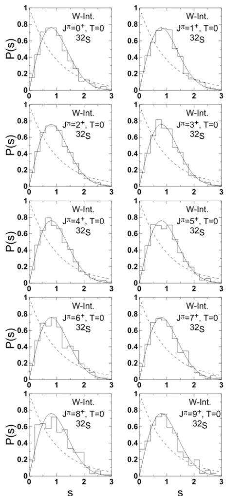
Figure 1. The nearest level spacing distributions in 32_{S nucleus for the}

states J Tπ =0 0 9 0.+ − + The histograms are the calculated with full hamiltonian. The solid and dashed lines are the GOE and Poisson distributions, respectively.

Figure 1 demonstrates the nearest-neighbors level spacing distributions P s( ), obtained with full hamiltonian calculations,

distribution (which corresponds to a random sequence of levels and describes regular systems) is displayed by the dashed line. The calculated distributions of P s( ) (histograms) for

0 0 7 0

J Tπ = + − + levels agree well with the GOE distribution. The level repulsion at small spacings produced through the mixing by the off-diagonal hamiltonian (which is considered as a distinctive feature of chaotic level statistics) is clearly seen in the calculated histograms. In spite of the level repulsion at small spacings in histograms J Tπ =8 0+ and 9 0+ levels is slightly decreased, the general performance of these histograms is still very close to the GOE limit. It is obvious from Figure 1 that the P s( ) (histograms) distribution is independent of the spin J _{(universal for different spins).}

Figure 2 shows the nearest-neighbors level spacing distributions P s( ), obtained with full hamiltonian calculations, for

T

=

1

and 2 nuclei. The distributions for Jπ =1 , 3+ + and 6+ _{states with}

T

=

1

(32P) and

T

=

2

(32Si) nuclei are presented in the upper and lower panels, respectively. It is clear that all selected states with

T

=

1

and

2

T

=

_{are in very good agreement with the GOE limit of} random matrices. It is found from this figure that the nearest neighbor level spacing distribution is independent of the isospin T.

Figure 2. The nearest level spacing distributions for the states

1 , 3

Jπ= + + and 6 .+ The upper panel corresponds to T=1 (32P ) and the lower panel corresponds to T=2 (32Si ) nuclei. The histograms correspond to the calculated with full Hamiltonian. The solid and dashed lines are the GOE and Poisson distributions, respectively.

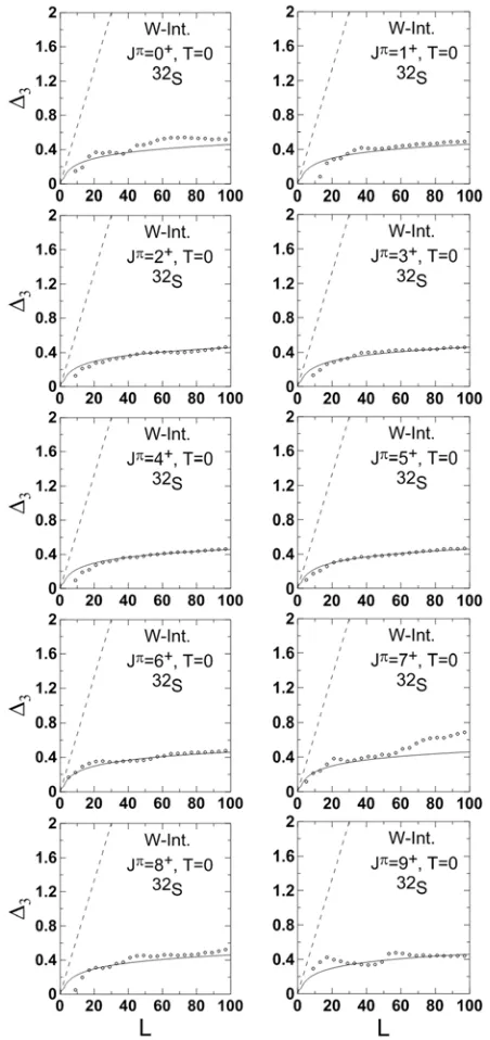
Figure 3 illustrates the spectral rigidity (Dyson’s ∆₃ statistics), obtained with full hamiltonian calculations, for the

0

T = (32S) nucleus. The calculated average ∆₃( )L statistic (denoted by open circles) is plotted as a function of

L

for various unfolded J Tπ =0 0 9 0+ − + states. The Poisson distribution (denoted by the dashed line) and the GOE distribution (denoted by the solid line) are also displayed for comparison. The calculated distributions of ∆₃ statistics for

0 0, 7 0

J Tπ = + + and 9 0+ states reveal some slight oscillations around the GOE distribution. These oscillations are attributed to the number of intervals n_α (which is

connected to the dimension of J Tπ states) used in averaging the statistics ∆₃( , ),α L see Eq. (11). A smooth statistics corresponds to a large n_α and non-smooth statistics

corresponds to a small n_α. Nevertheless, the global behavior

for calculated statistics of J Tπ =0 0, 7 0+ + and 9 0+ states is still very near to the GOE limit. In general, the calculated

3( )L

∆ statistics of all considered J Tπ =0 0 9 0+ − + states are found to have a chaotic behavior, in very good agreement with GOE of random matrices. Besides, they show no dependency on the spin J.

Figure 3. The average ∆₃ statistics in 32_{S nucleus for the states} 0 0 9 0.

Figure 4 exemplifies the Dyson’s ∆₃ statistics (the spectral rigidity), obtained with full hamiltonian calculations, for

T

=

1

and 2 nuclei. The average ∆₃ statistics for

1 , 3

Jπ = + + and 6+ _{states with}

T

=

1

(32P ) and

T

=

2

(32Si) nuclei are displayed in the upper and lower panels,

correspondingly. Again the ∆₃ statistics for all chosen states with

T

=

1

_{and are consistent with the GOE of the random}

matrix theory. It is so obvious from this figure that the

∆

₃ statistics are independent of the isospin

Figure 4. The average ∆₃ statistics for the states Jπ =1 , 3+ + and 6 .+ The upper panel corresponds to T=1 (32P ) and the lower panel corresponds to 2

T= (32Si ) nuclei. The open circles correspond to the calculated results with full Hamiltonian. The solid and dashed lines are the GOE and Poisson distributions, respectively.

It is important to denote that the calculated results for the

3

∆

statistics in Figures. 3 and 4 confirm the outcome of Figures. 1 and 2 that we have obtained from the analysis of the

P

(

s

)

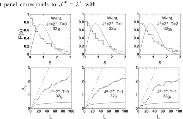
distributions.

Figure 5 shows the unperturbed hamiltonian results (the non-interacting particles case) for the distributions

(upper panel) and the average

∆

₃ statistics (lower panel).

The left panel corresponds to

J

π

=

2

+ with

T

=

0

(32

S

), the middle panel corresponds to

J

π

=

2

+ with

T

=

1

(32

P

) and the right panel corresponds to

J

π

=

2

+ with

2

=

T

( 32

Si

) nuclei. All calculated _(histograms) presented in the upper panel reveal regular behavior (in accordance with the Poisson distribution) due to the absence of mixing and repulsion between levels caused by the nonexistence of the off-diagonal residual interaction. The

lower panel of this figure shows the calculated

∆

₃ statistics (open circles) intermediate between the GOE (solid line) and the Poisson (dashed line) distributions. However, the calculated results for the average

∆

₃ statistics are closer to the Poisson distribution.

Figure 5. The distributions (upper panel) and the average ∆₃ statistics (lower panel) for Jπ=2 .+ The left panel corresponds to T=0 (32S ), the

4. Conclusions

The spectral fluctuations in A=32 nuclei are studied via the nuclear shell model. The sd-shell model calculations are accomplished by the OXBASH computer code with the isospin formalism interaction of W. The spectral fluctuations obtained with full hamiltonian calculations are found to be consistent with the GOE of random matrices (which characterizes the chaotic systems). Moreover, the distributions of

P

(

s

)

and ∆ statistics are found to be

independent of the spin

J

and isospin

T

.

For unperturbed hamiltonian calculations, we find a regular behavior for the distribution of

P

(

s

)

and an intermediate behavior between the GOE and the Poisson limits (closer to the Poisson limit) for the ∆ statistics. This regularity is attributed to the absence of the mixing and repulsion between levels as a result of the nonexistence of the off-diagonal residual interaction.

Acknowledgment

The authors would like to express their thanks to Professor B. A. Brown of the National Superconducting Cyclotron Laboratory, Micihigan State University, for providing the computer code OXBASH.

References

[1] F. Haak, Quantum signature of chaos, 2nd enlarged ed. (Springer-Verlag, Berlin, 2001).

[2] O. Bohigas, M. J. Giannoni and C. Schmit, Phys. Rev. Lett. 52, 1 (1986).

[3] S. Heusler, S. Muller, A. Altland, P. Braun, and F. Haak, Phys. Rev. Lett. 98, 044103 (2007).

[4] M. L. Mehta, Random Matrices, 3nd ed. (Academic, New York, 2004).

[5] T. Papenbrock, and H. A. Weidenmuller, Rev. Mod. Phys., Vol. 79, No. 3., 997 (2007).

[6] C. E. Porter, Statistical Theories of Spectra: Fluctuations (Academic, New York, 1965).

[7] T. A. Brody, J. Flores, J. B. French, P. A. Mello, A. Pandey and S. S. M. Wong, Rev. Mod. Phys. 53, 385 (1981).

[8] T. Guhr, A. Mü ller-Groeling and H. A. Weidenm ü ller, Phys. Rep. 299, 189 (1998).

[9] Y. Alhassid, Rev. Mod. Phys. 72, 895 (2000).

[10] M. C. Gutzwiller, Chaos in Classical and Quantum Mechanics (Springer-Verlag, New York, 1990).

[11] Y. Alhassid, A. Novoselsky and N. Whelan, Phys. Rev. Lett. 65, 2971 (1990); Y. Alhassid and N. Whelan, Phys. Rev. C 43, 2637 (1991).

[12] Y. Alhassid and A. Novoselsky, Phys. Rev. C 45, 1677 (1992). [13] Y. Alhassid and D. Vretenar, Phys. Rev. C 46, 1334 (1992). [14] V. Zelevinsky, B. A. Brown, N. frazier and M. Horoi, Phys.

Rep. 276, 85 (1996).

[15] R. R. Whitehead et al., Phys. Lett. B 76, 149 (1978).

[16] J. J. M. Verbaarschot and P. J. Brussaard, Phys. Lett. B 87, 155 (1979).

[17] B. A. Brown and G. Bertsch, Phys. Lett. B 148, 5(1984). [18] H. Dias et al., J. Phys. G 15, L79 (1989).

[19] V. Zelevinsky, M. Horoi and B. A. Brown, Phys. Lett. B 350, 141 (1995).

[20] A. Hamoudi, R. G. Nazmidinov, E. Shahaliev and Y. Alhassid, Phys. Rev. C65, 064311 (2002).

[21] P. W. M. Glaudemans, P. J. Brussaard and R. H. Wildenthal, Nucl. Phys. A 102, 593 (1976).

[22] A. Hamoudi, Nucl. Phys. A 849, 27 (2011).

[23] A. Hamoudi and A. Abdul Majeed Al-Rahmani, Nucl. Phys. A 892, 21 (2012).

[24] F. S. Stephens, M. A. Deleplanque, I. Y. Lee, A. O. Macchiavelli, D. Ward, P. Fallon, M. Cromaz, R. M. Clark, M. Descovich, R. M. Diamond, and E. Rodriguez-Vieitez, Phys. Rev. Lett., 94, 042501 (2005).

[25] A. B. Brown, A. Etchegoyen, N. S. Godin, W. D. M. Rae, W. A. Richter, W. E. Ormand, E. K. Warburton, J. S. Winfield, L. Zhao and C. H. Zimmermam, MSU-NSCL Report Number 1289.