A Hybrid Algorithm for Multi-Objective Optimization of Minimizing Makespan and Total Flow Time in Permutation Flow Shop Scheduling Problems

A Hybrid Algorithm for

Multi-Objective Optimization of

Minimizing Makespan and Total

Flow Time in Permutation Flow

Shop Scheduling Problems

ITC 1/48

Journal of Information Technology and Control

Vol. 48 / No. 1 / 2019 pp. 47-57

DOI 10.5755/j01.itc.48.1.20909

A Hybrid Algorithm for Multi-Objective Optimization of

Minimizing Makespan and Total Flow Time in Permutation

Flow Shop Scheduling Problems

Received 2018/06/08

Accepted after revision 2018/09/27

http://dx.doi.org/10.5755/j01.itc.48.1.20909

Corresponding author:

[email protected]

R. B. Jeen Robert

Faculty of Mechanical Engineering; AAA College of Engineering and Technology; Amathur, Sivakasi -626005,

India; phone: +91 9488081212; e-mail: [email protected]

R. Rajkumar

Faculty of Mechanical Engineering; Mepco Schlenk Engineering College; Sivakasi -626005, Virudhunagar Dist,

India; phone: +91 9486259435; e-mail: [email protected]

In this work, a hybrid algorithm has been proposed to solve bi-objective permutation flow shop scheduling

prob-lem. The primary concern of flow shop scheduling problem considered in this work is to obtain the best sequence,

which minimizes the makespan and the total flow time of all jobs. Bi-objective issues are comprehended by doling

out uniform weight to every objective function in view of its preference or determining every competent

solu-tions. In the flow shop scheduling environment, many meta-heuristic algorithms have been used to find optimal

or near-optimal solutions due to the computational cost of determining exact solutions. This work provides a

hy-bridization of genetic algorithm and simulated annealing algorithm (HGASA) based multi-objective optimization

algorithm for flow shop scheduling. The proposed HGASA algorithm is used to solve a bi-objective problem that

minimizes the makespan and the total flow time. The performance of the proposed algorithm is demonstrated by

applying it to benchmark problems available in the OR-Library. The test results show that the HGASA algorithm

performed better in terms of searching quality and efficiency than other meta-heuristic algorithms.

Information Technology and Control 2019/1/48

48

1. Introduction

In permutation flow shop scheduling, ‘

n

’ jobs must

be processed on ‘

m

’ machines in the same Order

se-quence. The operation succession is the same for all

jobs. The permutation flow shop scheduling (PFSSP)

has a broad foundation in assembling frameworks

and has pulled in numerous analysis consideration

by Johnson [10]. Numerous researches for single

ob-jective FSSPs result in a schedule to minimize the

makespan. The traditional ways to solve

single-objec-tive FSSP can be predominantly partitioned into two

classes, to be specific, exact and approximation

tech-niques. For a limited-wait constraints, complex

hy-brid flow-shop scheduling problem was solved with

discrete time exact arrangement approach by Gicquel

et al. [6], and a modified teaching–learning-based

op-timization algorithm has been used to solve

bi-objec-tive re-entrant hybrid flow shop scheduling by Shen

et al. [20]. Later, Jeen Robert and Rajkumar [8]

pro-posed a hybrid algorithm for minimizing makespan

in the PFSSP. Two-machine and three-machine flow

shop scheduling problem is solved using

branch-and-bound (B&B) algorithm [7]. Campbell et al. [4] built

up a heuristic algorithm for

n

-job m-machine

se-quencing problem with a goal of minimizing total flow

time. A general schedule for

n

jobs with m machines is

(n!)m

. In this situation, just

n!

schedules must be

con-sidered to stay away from job flow. The performance

measures of flow shop scheduling are makespan,

to-tal flow time and tardiness and so on. In flow shop

environment, solving a single objective problem is

very tedious one. Majority of studies for the flow shop

scheduling problem focuses to minimize makespan.

However, there are other important objectives than

makespan for the flow shop scheduling problem. For

example, the total flow time, the total machine idle

time are very important performance measures in

minimizing total scheduling cost. Hence, we consider

the flow shop scheduling problem with the objectives

of makespan and total flow time in this study. Weishi

et al. [23] described a self-guided differential

evolu-tion with a neighborhood search for permutaevolu-tion flow

shop scheduling. Rajendran [14] has developed a

heu-ristic algorithm with the objective of minimizing the

makespan and the total flow time for bi-objective flow

shop scheduling problem. Nagar et al. [11] developed a

combined hybrid algorithm to solve PFSSP with

bet-ter minimization of makespan and average total flow

Recently, Sanjeev Kumar et al. [19] developed a

mod-ified gravitational emulation local search (MGELS)

algorithm to minimize both makespan and total flow

time. The proposed methodology is carried out with

the flow shop benchmark problem, and the

execu-tion of MGELS algorithm is contrasted with CR

al-gorithm, HAMC1, HAMC2, HAMC3, CR (MC),

Mul-tiple Objective Adaptive Clonal Selection Algorithm

(MOACSA), GA, and DT algorithm. In this present

work, a hybrid algorithm is proposed that hybridizes

the Genetic Algorithm (GA) and the simulated

An-nealing (SA) algorithm. The Genetic algorithm acts

as local search scheme and the Simulated Annealing

algorithm acts as a global search scheme by accepting

some inferior count values. Moreover, in proposed

HGASA, the sub chromosomal level crossover and

mutation is implemented to get better results and

this seed is given to the SA algorithm to get further

improvements which avoids the worst solution. So it

is believed that HGASA can achieve satisfactory

im-provement for PFSSPs. Then the performance of the

proposed algorithm is tested with flow shop

schedul-ing benchmark problems. The results obtained by the

proposed HGASA are compared with earlier reported

results of CR algorithm, HAMC1, HAMC2, HAMC3,

CR (MC), MOACSA, GA, and DT algorithm. Test

re-sults show that the proposed algorithm is more

effi-cient than other algorithm and best suited for large

sized problems.

The rest of this paper is organized as follows: Section 2

presents the mathematical model of PFSP. Section 3

presents the flowchart and procedure of proposed

HGS-SA for PFSP. Section 4 shows the experimental results

and comparisons between HGSSA and other algorithms.

Section 5 summarizes the conclusions of this work.

2. Mathematical Model of PFSP

In the present paper, bi-objective optimization for

minimizing the makespan and total flow time for

es-tablished PFSP is considered. The detailed

explana-tion of PFSP is given in sub sequent secexplana-tion.

2.1. Permutation Flow Shop Scheduling

Problem (PFSP)

The main objective of the permutation flow shop

sched-uling problem is to find a suitable job sequence that

minimizes makespan and total flow time. The objective

of this work is to develop a HGASA and hence to find the

optimal or near optimal solution sequence in flow shop

scheduling by minimizing makespan and total flow

time. In PFSP, there are ‘

n’

independent jobs

(permuta-tion job set

j

= 1, 2,. . .n) that should be processed on ‘

m’

machines (

k

= 1,2,. . .m) and

B

is an inter-mediate buffer

between two consecutive machines

.

All the machines

(

M

, M

,…..,M

) follow the same job sequence till the

end of all operations. This means that, the

r

_{task of job}

j

is executed by machine

M

with processing time

T(r, j),

where 1

≤

r 

≤

m

, and 1 

≤

j 

≤

k.

Therefore, the completion

times of jobs on the machines, makespan and the total

flow time (TFT) of the jobs in the flow shop scheduling

can be intended as follows:

The following notations are used in PFSP:

T(r, j)

Processing time for job

r

on a given

ma-chine

j

(

r

=1, 2,…..n), (

j

= 1, 2…..m)

n

total number of jobs to be scheduled

m

total number of machines in the process

Cmax

makespan

r

the occupation sequenced in the

i

posi-tion of a schedule

C(r, j)

the completion time of jobs

r

on machine

j

The multi-objective flow shop scheduling problem

consists of scheduling

n

jobs with given processing

time on m machines. The flow shop problem has a

fun-damental assumption, i.e.

n

jobs are processed on m

machines in the same order. The initial machine setup

time is not considered for determining the makespan

value calculation. The following equations are used to

find the completion time of the job schedule:

C(1, 1)=

T(1, 1)

C(1, j)=

C(1, j-1)+ T(1, j)

C(r, 1)=

C(r-1, 1)+ T(r, 1)

C(r, j)=

Max(C(r,j-1), C(r-1,j))+T(r, j)

TFT=

1

( , ) n

i= C i m

∑

.

In Eq. (4),

T(r, j)

represents the finishing time of

r

_job

of the

j

_{work on machine}

_M

Information Technology and Control 2019/1/48

50

the finishing time of the

i

_{job in the last machine ‘m’,}

i.e. Total flow time (TFT) is the total completion time

of all jobs spent on the production system.

3. The Proposed Hybrid Algorithm

(HGASA)

We proposed a hybrid (HGASA) meta-heuristic

al-gorithm, which can be used for the minimization of

makespan and total flow time in the PFSP.

Hybridiza-tion indicates combining of two or more algorithms

to solve a given complex problem. Our algorithm

hy-bridizes the Genetic Algorithm and the simulated

an-nealing algorithm to reach global best (gbest) or near

to global solution. In HGASA, Genetic Algorithm acts

as local search scheme, and the Simulated Annealing

algorithm acts as global search scheme by accepting

some inferior count values. Moreover, in the proposed

HGASA, the sub chromosomal level crossover and

mutation are implemented to get better results, and

this seed is given to SA algorithm to get further

im-provements by avoiding worst solution. As a result, it

is believed that HGASA can achieve satisfactory

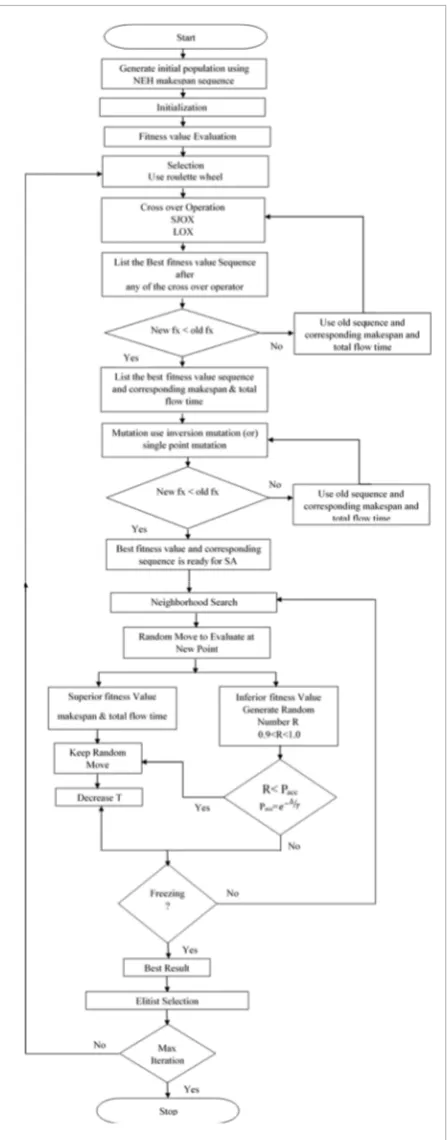
im-provement in PFSPs. The framework for the HGASA

algorithm to the Permutation Flow Shop Scheduling

Problem is clearly illustrated in Fig. 1. for the

bi-ob-jective optimization of makespan and total flow time

minimization. The steps involved in the proposed

HGASA algorithm are stated below.

Step 1:

Generate an initial population using Nawaz et

al. [12] (NEH) algorithm.

Step 2:

Initialization; Define the size of population =

1500; number of generations =200; crossover

proba-bility=0.05; mutation probability=0.05.

Step 3: Evaluate the Fitness function value of each

chromosome by

max

1 ( )

1 (0.5 0.5 ) f x

C TFT

=

+ +

, where

C

= makespan and TFT=

C(i, m)

.

Step 4:

Perform the following crossover

opera-tion: list the best

f(x)

sequence that minimizes both

makespan and total flow time.

Similar Job Order Crossover (SJOX)

SJOX crossover is based on the idea of identifying

and maintaining building blocks in the offspring.

In this way similar blocks or occurrences of jobs in

Figure 1

Table 1

Similar Job Order Crossover (SJOX)

Parent1 3 5 6 4 2 7 8 9 1

Offspring1 3 5 6 4 2 9 8 7 1

Offspring2 3 9 8 4 2 5 6 7 1

Parent2 3 9 8 4 2 5 7 6 1

cut point

Step 2.

Produce a proto-offspring by copying the

sub-section sequence into the corresponding positions of it.

Step 3.

Delete the operations which are already in the

subsequence from the second parent. The resulted

se-quence of operations contains the operations that the

proto-offspring needs.

Step 4.

Place the operations into the unfixed positions

of the proto-offspring from left to right according to

the order of the sequence to produce an offspring.

Step 5:

Mutation produces an offspring arrangement

by arbitrarily altering the parent’s qualities. In this

present algorithm, two different types of mutation

op-erators are introduced, namely inverse mutation and

single point mutation.

Inverse Mutation

In a sequence, two positions

i

and

j

are randomly

se-lected. The portion of the sequence between these

two positions is inverted to get a new mutated

se-quence. The new sequence represents the sequence

of operations after mutation. If the makespan of the

mutated sequence is less than the makespan of the

original sequence, the old sequence is replaced by

the new sequence. (Example. Mutation positions

be-tween 2 and 8).

Original Sequence

8 9 7 6 4 5 3

2 1

Mutated Sequence

8 4 3 2 7 9 6

5 1

Single Point Mutation

A random operation is selected in the sequence and

moved to another random position in the sequence.

If the makespan of the resulting sequence is less than

that of the previous one, it replaces the previous

se-quence.

Before single point mutation

8 9 7 6 4 5 3

2 1

After single point mutation

8 9 7 4 5 3 2

1 6

Step 6: Simulated annealing begins with a

neighbor-hood search by defining initial parameters.

both parents are passed over to child unaltered. If

there are no similar blocks in the parents the

cross-over operator will behave like the single-point order

crossover. The SJOX crossover operator can be

ex-plained as follows:

Step 1:

Both parents are examined on a

posi-tion-by-position basis. Identical jobs at the same

po-sitions are copied over to both offspring.

Step 2:

The offspring directly inherits all jobs from

the corresponding parents up to a randomly chosen

cut point. That is, Child1 inherits directly from

Par-ent1 and Child2 from Parent2.

Step 3:

Missing elements at each offspring are

cop-ied in the relative order of the other parent and it is

shown in Table 1.

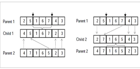
Linear Order Crossover (LOX)

Linear Order Crossover (LOX) tries to preserve both

the relative positions between genes as much as

pos-sible and the absolute positions relative to the

ex-tremities of parents and it is shown in Fig. 2.

Figure 2

Linear order crossover

Information Technology and Control 2019/1/48

52

Step 7: Random move to evaluate at the new point.

The obtained fitness function values are compared

with existing fitness function values. If the obtained

value is the superior one, then repeat the same

pro-cess to get further better results. The advantage of the

simulated annealing process is that the inferior

solu-tions are also accepted to get the global best value.

The probability of inferior value acceptance is

mea-sured by

Linear Order Crossover (LOX) tries to preserve both the relative positions between genes as much as possible and the absolute positions relative to the extremities of parents and it is shown in Fig. 2. Step 1. Select a subsequence of operations from one parent at random.

Step 2. Produce a proto-offspring by copying the subsection sequence into the corresponding positions of it.

Step 3. Delete the operations which are already in the subsequence from the second parent. The resulted sequence of operations contains the operations that the proto-offspring needs.

Step 4. Place the operations into the unfixed positions of the proto-offspring from left to right according to the order of the sequence to produce an offspring.

Figure 2 Linear order crossover

Step 5: Mutation produces an offspring arrangement by arbitrarily altering the parent’s qualities. In this present algorithm, two different types of mutation operators are introduced, namely inverse mutation and single point mutation.

Inverse Mutation

In a sequence, two positions i and j are randomly selected. The portion of the sequence between these two positions is inverted to get a new mutated sequence. The new sequence represents the sequence of operations after mutation. If the makespan of the mutated sequence is less than the makespan of the original sequence, the old sequence is replaced by the new sequence. (Example. Mutation positions between 2 and 8). Original Sequence

8 9 7 6 4 5

3 2 1

Mutated Sequence

8 4 3 2 7 9

6 5 1

Single Point Mutation

A random operation is selected in the sequence and moved to another random position in the

sequence. If the makespan of the resulting sequence is less than that of the previous one, it replaces the previous sequence.

Before single point mutation

8 9 7 6 4

5 3 2 1

After single point mutation

8 9 7 4 5

3 2 1 6

Step 6: Simulated annealing begins with a neighborhood search by defining initial parameters.

Step 7: Random move to evaluate at the new point. The obtained fitness function values are compared with existing fitness function values. If the obtained value is the superior one, then repeat the same process to get further better results. The advantage of the simulated annealing process is that the inferior solutions are also accepted to get the global best value. The probability of inferior

value acceptance is measured by

) (

T acc

P

=

e

where ∆ is objective difference = (f(x’)-f(x)), where 𝑥𝑥𝑥𝑥𝑖𝑖𝑖𝑖𝑖𝑖𝑖𝑖 𝑡𝑡𝑡𝑡ℎ𝑒𝑒𝑒𝑒𝑐𝑐𝑐𝑐𝑐𝑐𝑐𝑐𝑐𝑐𝑐𝑐𝑐𝑐𝑐𝑐𝑒𝑒𝑒𝑒𝑐𝑐𝑐𝑐𝑡𝑡𝑡𝑡 𝑚𝑚𝑚𝑚𝑚𝑚𝑚𝑚𝑚𝑚𝑚𝑚𝑒𝑒𝑒𝑒𝑖𝑖𝑖𝑖𝑚𝑚𝑚𝑚𝑚𝑚𝑚𝑚𝑐𝑐𝑐𝑐, 𝑥𝑥𝑥𝑥′ 𝑖𝑖𝑖𝑖𝑖𝑖𝑖𝑖 𝑡𝑡𝑡𝑡ℎ𝑒𝑒𝑒𝑒 𝑐𝑐𝑐𝑐𝑒𝑒𝑒𝑒𝑖𝑖𝑖𝑖𝑛𝑛𝑛𝑛ℎ𝑏𝑏𝑏𝑏𝑏𝑏𝑏𝑏𝑐𝑐𝑐𝑐ℎ𝑏𝑏𝑏𝑏𝑏𝑏𝑏𝑏𝑜𝑜𝑜𝑜𝑏𝑏𝑏𝑏𝑜𝑜𝑜𝑜𝑥𝑥𝑥𝑥 and T is the temperature. In the proposed HGASA algorithm, the random number is generated in the range of 0.9 to 1.

Step 8: Check for freezer count by reducing the system temperature according to the cooling schedule.

Step 9: List the best fitness function value and corresponding sequence by indicating makespan and total flow time.

Step 10: The procedure is stopped when the temperature reaches the final set temperature or it reach the maximum number of iterations.

4.

Experimental Results and

Comparisons

In this article, the proposed HGASA algorithm is coded in Matlab 2009 programming tool and tried on an Intel Core i-3, 1.6 GHz with 4 GB RAM PC equipment. It has been tried with 28 flow shop benchmark problems, jobs sizes from 20, 50, and 100 and machines sizes from 5, 10, and 20. These benchmark problems are taken from Taillard [21]. Each instance can be characterized by the following parameters:

where

∆

is objective difference

=

(f(x’)-f(x)),

where

𝑥

𝑖𝑠

𝑡ℎ𝑒

𝑐𝑢𝑟𝑟𝑒𝑛𝑡

𝑚𝑎𝑘𝑒𝑠𝑝𝑎𝑛

,

𝑥

′

𝑖𝑠

𝑡ℎ𝑒

𝑛𝑒𝑖𝑔ℎ𝑏𝑜𝑟ℎ𝑜𝑜𝑑

𝑜𝑓

𝑥

and T is the temperature. In

the proposed HGASA algorithm, the random number

is generated in the range of 0.9 to 1.

Step 8:

Check for freezer count by reducing the

sys-tem sys-temperature according to the cooling schedule.

Step 9:

List the best fitness function value and

corre-sponding sequence by indicating makespan and total

flow time.

Step 10:

The procedure is stopped when the

tempera-ture reaches the final set temperatempera-ture or it reach the

maximum number of iterations.

4. Experimental Results and

Comparisons

In this article, the proposed HGASA algorithm is

cod-ed in Matlab 2009 programming tool and tricod-ed on an

Intel Core i-3, 1.6 GHz with 4 GB RAM PC equipment.

It has been tried with 28 flow shop benchmark

prob-lems, jobs sizes from 20, 50, and 100 and machines

sizes from

5, 10, and 20. These benchmark problems

are taken from Taillard [21]. Each instance can be

characterized by the following parameters: number of

jobs (

n

) and number of machines (

m

). Each instance

has been subjected for 200 iterations to find the best

fitness function value. The performance analysis of

the proposed HGASA algorithm is described in

Ta-ble 2. Equal weights are considered for each objective

(0.5, 0.5) as the MS and TFT objectives are

conflict-ing in nature. The equal weights are considered in

Yagmahan and Yenisey [22] and Balasundaram et al.

[3]. Considering makespan as an objective, 28

bench-mark problems have been solved. Out of these

prob-lems, HGASA algorithm produced 16 best makespan

solutions, whereas MGELS algorithm produced 8

best solutions. Decision Tree algorithm produced one

best solution, and CR (MC) produced three best

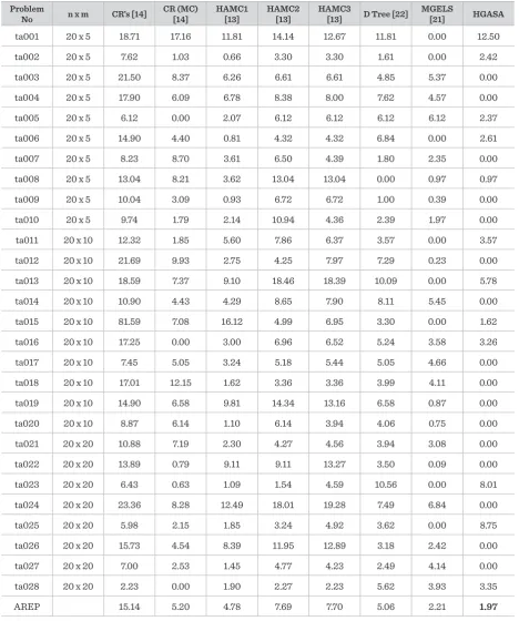
solu-tions. Table 3 gives the percentage improvement in

makespan value using HGASA over earlier literature

results. Moreover, the Average Relative Error

Per-centage (AREP) of the proposed HGASA algorithm

is (1.97) less than that of all different methodologies

such as MGELS, DT algorithm, HAMC3, HAMC2,

HAMC1, CR (MC), and CR in view of makespan

ob-jective and it is shown in Fig. 3. The performance of

the algorithms is given using Average Relative Error

Percentage (AREP) equation

max

1 ( )

1 (0.5 0.5 )

f x

C TFT

=

+ +

,

where

C*

is the Best makespan.

Figure 3

A comparison of AREP of HGASA algorithm with other methods for makespan

Table 2

Performance analysis of the proposed HGASA algorithm method with the existing methods

Prob-lem No

CR’s [14] CR (MC) [14] HAMC1 [13] HAMC2 [13] HAMC3 [13] Decision Tree _[22] MGELS [21] HGASA

MS TFT MS TFT MS TFT MS TFT MS TFT MS TFT MS TFT MS TFT

ta001 1377 14,361 1359 15,196 1297 14,274 1324 14,150 1307 14,193 1297 14105 1160 14220 1305 14199 ta002 1468 15,947 1378 18,204 1373 16,483 1409 15,386 1409 15,386 1386 15403 1364 15354 1397 15405 ta003 1379 14,261 1230 15,697 1206 13,858 1210 13,798 1210 13,798 1190 13759 1196 13464 1135 13973 ta004 1548 16,268 1393 17,037 1402 16,086 1423 15,770 1418 15,773 1413 15652 1373 15569 1313 16106 ta005 1387 19,884 1307 15,429 1334 14,897 1387 13,771 1387 13,779 1387 13726 1387 13660 1338 13619 ta006 1411 14,251 1282 15,030 1238 13,853 1281 13,389 1281 13,413 1312 13732 1228 13582 1260 13179 ta007 1381 13,972 1387 15,925 1322 14,215 1359 13,955 1332 13,959 1299 13872 1306 13838 1276 13867 ta008 1404 14,278 1344 15,716 1287 14,405 1404 14,269 1404 14,278 1242 14133 1254 14469 1254 14185 ta009 1425 14,907 1335 15,556 1307 15,823 1382 14,835 1382 14,835 1308 14863 1300 14660 1295 14600 ta010 1284 13,374 1191 14,622 1195 13,676 1298 13,204 1221 13,232 1198 13185 1193 13382 1170 13320 ta011 1887 22,526 1711 23,125 1774 22,427 1812 22,202 1787 22,234 1740 22078 1680 21298 1740 21327 ta012 2121 24,139 1916 26,526 1791 23,461 1817 23,003 1832 23,046 1870 22927 1747 23025 1743 23113 ta013 1786 20,654 1617 21,572 1643 21,818 1784 20,577 1783 20,608 1658 20600 1506 20156 1593 20148 ta014 1628 19,440 1533 20,761 1531 19,599 1595 19,276 1584 19,332 1587 19058 1548 18952 1468 19190 ta015 2693 34,484 1588 20,875 1722 19,740 1557 20,510 1586 19,463 1532 19373 1483 18975 1507 18875 ta016 1835 20,861 1565 21,109 1612 20,064 1674 19,751 1667 19,846 1647 19758 1621 19952 1616 19552 ta017 1659 19,422 1622 20,306 1594 19,268 1624 18,718 1628 18,992 1622 18967 1616 19007 1544 18850 ta018 1878 21,336 1800 23,991 1631 21,596 1659 20,958 1659 21,049 1669 20815 1671 21163 1605 20928 ta019 1851 20,859 1717 22,572 1769 21,595 1842 20,823 1823 20,851 1717 20903 1625 20767 1611 20972 ta020 1878 21,901 1831 25,034 1744 21,819 1831 21,541 1793 21,573 1795 21817 1738 20793 1725 21000 ta021 2700 35,405 2610 38,650 2491 36,027 2539 34,907 2546 35,159 2531 34830 2510 34638 2435 34404 ta022 2600 34,326 2301 35,426 2491 33,304 2491 33,304 2586 34,319 2363 32749 2285 32804 2283 32266 ta023 2550 33,519 2411 35,152 2422 33,556 2433 32,900 2506 33,411 2649 34328 2396 32857 2588 34411 ta024 2815 36,130 2471 37,081 2567 37,870 2693 35,475 2722 35,810 2453 32689 2438 32635 2282 31987 ta025 2518 33,729 2427 35,285 2420 35,029 2453 33,198 2493 33,682 2462 35735 2376 33137 2584 33320 ta026 2730 35,135 2466 37,142 2557 36,712 2641 34,742 2663 35,089 2434 34035 2416 34017 2359 33267 ta027 2582 33,025 2174 36,126 2448 34,389 2528 33,402 2515 33,484 2473 33615 2013 33362 2434 33569 ta028 2472 33,526 2418 34,076 2464 33,565 2473 33,479 2472 33,500 2554 33321 2513 33583 2499 33534

Information Technology and Control 2019/1/48

54

Table 3

Percentage improvement in makespan value using HGASA over earlier literature results

Problem

No n x m CR’s [14] CR (MC) [14] HAMC1 [13] HAMC2 [13] HAMC3 [13] D Tree [22] MGELS [21] HGASA

ta001 20 x 5 18.71 17.16 11.81 14.14 12.67 11.81 0.00 12.50

ta002 20 x 5 7.62 1.03 0.66 3.30 3.30 1.61 0.00 2.42

ta003 20 x 5 21.50 8.37 6.26 6.61 6.61 4.85 5.37 0.00

ta004 20 x 5 17.90 6.09 6.78 8.38 8.00 7.62 4.57 0.00

ta005 20 x 5 6.12 0.00 2.07 6.12 6.12 6.12 6.12 2.37

ta006 20 x 5 14.90 4.40 0.81 4.32 4.32 6.84 0.00 2.61

ta007 20 x 5 8.23 8.70 3.61 6.50 4.39 1.80 2.35 0.00

ta008 20 x 5 13.04 8.21 3.62 13.04 13.04 0.00 0.97 0.97

ta009 20 x 5 10.04 3.09 0.93 6.72 6.72 1.00 0.39 0.00

ta010 20 x 5 9.74 1.79 2.14 10.94 4.36 2.39 1.97 0.00

ta011 20 x 10 12.32 1.85 5.60 7.86 6.37 3.57 0.00 3.57

ta012 20 x 10 21.69 9.93 2.75 4.25 7.97 7.29 0.23 0.00

ta013 20 x 10 18.59 7.37 9.10 18.46 18.39 10.09 0.00 5.78

ta014 20 x 10 10.90 4.43 4.29 8.65 7.90 8.11 5.45 0.00

ta015 20 x 10 81.59 7.08 16.12 4.99 6.95 3.30 0.00 1.62

ta016 20 x 10 17.25 0.00 3.00 6.96 6.52 5.24 3.58 3.26

ta017 20 x 10 7.45 5.05 3.24 5.18 5.44 5.05 4.66 0.00

ta018 20 x 10 17.01 12.15 1.62 3.36 3.36 3.99 4.11 0.00

ta019 20 x 10 14.90 6.58 9.81 14.34 13.16 6.58 0.87 0.00

ta020 20 x 10 8.87 6.14 1.10 6.14 3.94 4.06 0.75 0.00

ta021 20 x 20 10.88 7.19 2.30 4.27 4.56 3.94 3.08 0.00

ta022 20 x 20 13.89 0.79 9.11 9.11 13.27 3.50 0.09 0.00

ta023 20 x 20 6.43 0.63 1.09 1.54 4.59 10.56 0.00 8.01

ta024 20 x 20 23.36 8.28 12.49 18.01 19.28 7.49 6.84 0.00

ta025 20 x 20 5.98 2.15 1.85 3.24 4.92 3.62 0.00 8.75

ta026 20 x 20 15.73 4.54 8.39 11.95 12.89 3.18 2.42 0.00

ta027 20 x 20 7.00 2.53 1.45 4.77 4.23 2.49 4.14 0.00

ta028 20 x 20 2.23 0.00 1.90 2.27 2.23 5.62 3.93 3.35

AREP 15.14 5.20 4.78 7.69 7.70 5.06 2.21 1.97

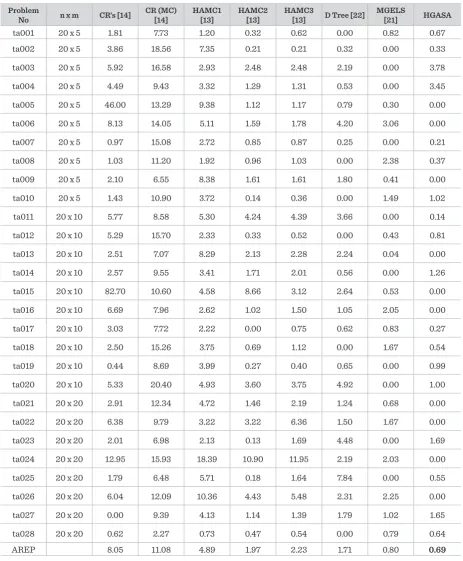
Table 4

Percentage improvement in total flow time value using HGASA over earlier literature results

Problem

No n x m CR’s [14] CR (MC) [14] HAMC1 [13] HAMC2 [13] HAMC3 [13] D Tree [22] MGELS [21] HGASA

ta001 20 x 5 1.81 7.73 1.20 0.32 0.62 0.00 0.82 0.67

ta002 20 x 5 3.86 18.56 7.35 0.21 0.21 0.32 0.00 0.33

ta003 20 x 5 5.92 16.58 2.93 2.48 2.48 2.19 0.00 3.78

ta004 20 x 5 4.49 9.43 3.32 1.29 1.31 0.53 0.00 3.45

ta005 20 x 5 46.00 13.29 9.38 1.12 1.17 0.79 0.30 0.00

ta006 20 x 5 8.13 14.05 5.11 1.59 1.78 4.20 3.06 0.00

ta007 20 x 5 0.97 15.08 2.72 0.85 0.87 0.25 0.00 0.21

ta008 20 x 5 1.03 11.20 1.92 0.96 1.03 0.00 2.38 0.37

ta009 20 x 5 2.10 6.55 8.38 1.61 1.61 1.80 0.41 0.00

ta010 20 x 5 1.43 10.90 3.72 0.14 0.36 0.00 1.49 1.02

ta011 20 x 10 5.77 8.58 5.30 4.24 4.39 3.66 0.00 0.14

ta012 20 x 10 5.29 15.70 2.33 0.33 0.52 0.00 0.43 0.81

ta013 20 x 10 2.51 7.07 8.29 2.13 2.28 2.24 0.04 0.00

ta014 20 x 10 2.57 9.55 3.41 1.71 2.01 0.56 0.00 1.26

ta015 20 x 10 82.70 10.60 4.58 8.66 3.12 2.64 0.53 0.00

ta016 20 x 10 6.69 7.96 2.62 1.02 1.50 1.05 2.05 0.00

ta017 20 x 10 3.03 7.72 2.22 0.00 0.75 0.62 0.83 0.27

ta018 20 x 10 2.50 15.26 3.75 0.69 1.12 0.00 1.67 0.54

ta019 20 x 10 0.44 8.69 3.99 0.27 0.40 0.65 0.00 0.99

ta020 20 x 10 5.33 20.40 4.93 3.60 3.75 4.92 0.00 1.00

ta021 20 x 20 2.91 12.34 4.72 1.46 2.19 1.24 0.68 0.00

ta022 20 x 20 6.38 9.79 3.22 3.22 6.36 1.50 1.67 0.00

ta023 20 x 20 2.01 6.98 2.13 0.13 1.69 4.48 0.00 1.69

ta024 20 x 20 12.95 15.93 18.39 10.90 11.95 2.19 2.03 0.00

ta025 20 x 20 1.79 6.48 5.71 0.18 1.64 7.84 0.00 0.55

ta026 20 x 20 6.04 12.09 10.36 4.43 5.48 2.31 2.25 0.00

ta027 20 x 20 0.00 9.39 4.13 1.14 1.39 1.79 1.02 1.65

ta028 20 x 20 0.62 2.27 0.73 0.47 0.54 0.00 0.79 0.64

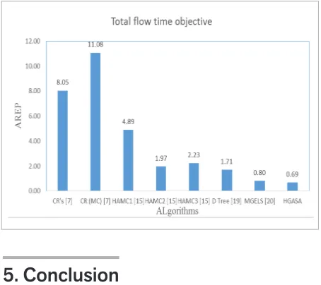
AREP 8.05 11.08 4.89 1.97 2.23 1.71 0.80 0.69

Information Technology and Control 2019/1/48

56

The performance of the algorithms is given using

Av-erage Relative Error Percentage (AREP) equation

AREP

(

min(

solutions C

_C

_*

)

*

) 100%

x

−

=

min(

)

*

(

) 100%

*

solutions D

AREP

x

D

−

=

where

D*

is the Best flow time value.

Figure 4

A comparison of AREP of HGASA algorithm with other methods for Total flow time

5. Conclusion

In this work, HGASA based meta-heuristic approach

is presented for bi-criteria optimization of

minimiz-ing makespan and total flow time simultaneously. It

is a well-known combinatorial for permutation flow

shop problem. The proposed algorithm is tested with

28 benchmark problems available in the literature

and the results are compared. As a bi-criteria model,

the proposed approach gives the best solution

com-pared to the existing methods. Unlike the existing

algorithms available for PFSP, to reach the global

best solution, initially GA background is used to get

a local best solution in the proposed algorithm.

Lat-er, the solution obtained through GA is given as input

for SA algorithm, subjecting to neighborhood search

by accepting some inferior count values to reach the

global best solution. Measurable results of numerous

problems of different sizes have demonstrated that

the proposed technique meets or beats the other

algo-rithms available in the literature. Progressive

applica-tions, more information and characteristics are

gath-ered in shop floor control system and Hybrid Genetic

Algorithm and Simulated Annealing algorithm will

lead to better dispatching rules, while, it is difficult

to evoke every single important part of the planning

to alternate methodologies. The results of our

perfor-mance measurement also revealed that the proposed

HGASA algorithm outperformed the meta-heuristics

in minimizing the makespan and total flow time.

In future, it could be added with more objectives such

as machine idle time, total tardiness, total work load,

and so on. Moreover, to solve permutation flow shop

scheduling problems with other hybrid approaches

is also more interesting. In addition, the HGASA

al-gorithm could be applied to solve other combinatorial

problems such as layout problems, job shop

schedul-ing, flexible job shop scheduling and flexible

manu-facturing system scheduling problems.

References

1. Abdolrazzagh Nezhada, M., Abdullah, S. Robust Intelli-gent Construction Procedure for Job-Shop Scheduling. Information Technology and Control, 2014, 43(3), 217-229. https://doi.org/10.5755/j01.itc.43.3.3536

2. Allouche, M. A., Aouni, B., Martel, J. M. Solving Multi-Criteria Scheduling Flow Shop Problem Through Compromise Programming and Satisfaction Functions. European Journal of Operational Research, 2009, 192(2), 460-467. https://doi.org/10.1016/j.ejor.2007.09.038 3. Balasundaram, R., Valavan, D., Baskar, N. Comparison

of Two Heuristic Approaches for Solving the Produc-tion Scheduling Problem. InformaProduc-tion Technology and

Control, 2010, 40(2), 118-122. https://doi.org/10.5755/ j01.itc.40.2.426

4. Campbell, H. G., Dudek, R. A., Smith, M. L. A Heuristic Algorithm for the n-Job m-Machine Sequencing Prob-lem. Manage Science, 1970, 16(16), 630-637. https://doi. org/10.1287/mnsc.16.10.B630

5. Ding, J.-Y., Song, S., Wu, C. Carbon-Efficient Scheduling of Flow Shops by Multi-Objective Optimization. Eu-ropean Journal of Operational Research, 2016, 248(3), 758-771.https://doi.org/10.1016/j.ejor.2015.05.019 6. Gicquel, C., Hege, L., Minoux, M., Van Canneyt, W. A

Hy-brid Flow-Shop Scheduling Problem with Limited-Wait Constraints. Computers and Operations Research, 2012, 39(3), 629-636. https://doi.org/10.1016/j.cor.2011.02.017 7. Ignall, E., Schrage, L. Application of the Branch and

Bound Technique to Some Flow Shop Scheduling Problems. Operations Research, 1965, 13 (3), 400-412. https://doi.org/10.1287/opre.13.3.400

8. Jeen Robert, R. B., Rajkumar, R. A Hybrid Algorithm for Minimizing Makespan in the Permutation Flow Shop Scheduling Environment. Asian Journal of Research in Social Sciences and Humanities, 2016, 6(9), 1239-1255. https://doi.org/10.5958/2249-7315.2016.00867.4 9. Jeen Robert, R. B., Rajkumar, R. An Effective

Genet-ic Algorithm for Flow Shop Scheduling Problems to Minimize Makespan. Mechanika, 2017, 23(4), 594-603. https://doi.org/10.5755/j01.mech.23.4.15053

10. Johnson, S. M. Optimal Two- and Three-Stage Produc-tion Schedules with Setup Times Included. Naval Re-search Logistics Quarterly, 1954, 1(1), 61-68. https://doi. org/10.1002/nav.3800010110

11. Nagar, A., Heragu, S. S., Haddock, J. A Combined Branch-and-Bound and Genetic Algorithm Based Ap-proach for a Flow Shop Scheduling Problem. Annals of Operations Research, 1996, 63(3), 397-414. https://doi. org/10.1007/BF02125405

12. Nawaz, M., Enscore, E., Ham, I. A Heuristic Algo-rithm for the m-Machine, n-Job Flowshop Sequenc-ing Problem. Omega, 1983, 11(1), 91-95. https://doi. org/10.1016/0305-0483(83)90088-9

13. Rajendran, C., Ziegler, H. A Multi-Objective Ant-Col-ony Algorithm for Permutation Flow Shop Schedul-ing to Minimize the Makespan and Total Flow Time of Jobs. Computational Intelligence in Flow Shop and Job Shop Scheduling, 2009, 230, 53-99. https://doi. org/10.1007/978-3-642-02836-6_3

14. Rajendran, C. Heuristics for Scheduling in Flow Shop with Multiple Objectives. European Journal of Op-erational Research, 1995, 82(3), 540-555. https://doi. org/10.1016/0377-2217(93)E0212-G

15. Rajendran, C., Ziegler, H. Ant-Colony Algorithms for Permutation Flow Shop Scheduling to Minimize Makespan and Total Flow Time of Jobs. European Jour-nal of OperatioJour-nal Research, 2004, 155(2), 426-438. https://doi.org/10.1016/S0377-2217(02)00908-6 16. Rajkumar, R., Shahabudeen, P. An Improved Genetic

Al-gorithm for the Flowshop Scheduling Problem. Interna-tional Journal of Production Research, 2009, 47(1), 233-249. https://doi.org/10.1080/00207540701523041

17. Rajkumar, R., Shahabudeen, P. Bi-Criteria Improved Genetic Algorithm for Scheduling in Flowshops to Mi-nimise Makespan and Total Flowtime of Jobs. Interna-tional Journal of Computer Integrated Manufacturing, 2009, 22(10), 987-998. https://doi.org/10.1080/095119 2090299335318.

18. Ravindran, D., Noorul Haq, A., Selvakuar, S. J. Flow Shop Scheduling with Multiple Objective of Minimiz-ing Makespan and Total Flow Time. The International Journal of Advanced Manufacturing Technology, 2005, 25(9), 1007-1012. https://doi.org/10.1007/s00170-003-1926-1

19. Sanjeev Kumar, R., Padmanaban, K. P., Rajkumar, M. Minimizing Makespan and Total Flow Time in Permu-tation Flow Shop Scheduling Problems Using Modified Gravitational Emulation Local Search Algorithm. Pro-ceedings of the Institution of Mechanical Engineers, Part B: Journal of Engineering Manufacture, 2016. https://doi.org/10.1177/0954405416645775

20. Shen, J.-N., Wang, L., Zheng, H.-Y. A Modified Teach-ing–Learning-Based Optimization Algorithm for Bi-Objective Re-Entrant Hybrid Flowshop Scheduling. International Journal of Production Research, 2015, 54(12), 3622-3639. https://doi.org/10.1080/00207543. 2015.1120900

21. Taillard, E. Benchmarks for Basic Scheduling In-stances. European Journal of Operational Research, 1993, 64(2), 278-285. https://doi.org/10.1016/0377-2217(93)90182-M

22. Wang, L., Pan, Q. K., Fatih Tasgetiren, M. A Hybrid Harmony Search Algorithm for the Blocking Permu-tation Flow Shop Scheduling Problem. Computers & Industrial Engineering, 2011, 61(1), 76-83. https://doi. org/10.1016/j.cie.2011.02.013

23. Weishi, S., Dechang, Pi. A Self-Guided Differential Evolution with Neighborhood Search for Permutation Flow Shop Scheduling. Expert Systems with Applica-tions, 2016, 51(1), 161-176. https://doi.org/10.1016/j. eswa.2015.12.001

24. Yagmahan, B., Yenisey, M. A Multi-Objective Ant Colo-ny System Algorithm for Flow Shop Scheduling Prob-lem. Expert Systems with Applications, 2010, 37(2), 1361-1368. https://doi.org/10.1016/j.eswa.2009.06.105 25. Yeh, W. C. An Efficient Branch-and-Bound Algorithm