Application and Comparison of the Intelligent Algorithms to Solve
the Fractional Heat Conduction Inverse Problem
Rafał Brociek
*, Damian Słota
Institute of Mathematics, Silesian University of Technology, Kaszubska 23, 44-100 Gliwice, Poland
e-mail: [email protected]
http://dx.doi.org/10.5755/j01.itc.45.2.13716
Abstract. This paper describes an application of intelligent algorithms to reconstruct the boundary condition of the second kind in the fractional heat conduction equation. For this purpose, a functional defining the error of approximate solution must be minimized. To minimize this functional two Ant Colony Optimization (ACO) algorithms were used and compared. In order to reduce the computational time, the calculations were performed in a parallel (multi-threaded) way. The paper presents also some examples to illustrate the accuracy and stability of the presented algorithms.
Keywords: Intelligent Algorithm, Ant Colony Optimization Algorithm, Inverse Problem, Identification, Time Fractional Heat Conduction Equation.
* Corresponding author; e-mail: [email protected]
1. Introduction
In many fields of science the inverse problems are some of the most important issues. They have found the wide applications in various disciplines, for example, in physics, control theory or signal processing, since the solutions of the inverse problems allow to fit properly the input parameters of considered model on the basis of the observational output results [12-15]. In this paper the inverse problem of the fractional heat conduction equation [4,5] is investigated in which, basing on the temperature measurements, the heat flux occurring in boundary condition is reconstructed.
Recently, in solving various practical and theoretical problems the artificial intelligence algorithms have been used [1,8,12-15,21,32,36-40]. Considering the artificial intelligence algorithms we can distinguish, among them, the optimization algorithms based on the natural behavior of insects, like for example the Artificial Bee Colony algorithm [16–18,30], the Ant Colony Optimization algorithm [10,11,34] or the firefly algorithm [32]. The main advantage of optimization algorithms grounded on the artificial intelligence is the fact that they do not need any requirements, except the existence of the solution of discussed problem. Moreover, in many cases these
algorithms provide better results than the conventional methods and are also easier to implement.
Many different types of physical and technical phenomena is modeled lately with the aid of the fractional order derivatives [6,7,9,19,22,29,31]. For example, we can find the applications of fractional derivative in electrical engineering [23], control sciences [6,9] and mechanics [7]. It happens quite often that the mathematical models expressed by means of the fractional order derivatives describe the discussed process better than the conventional models derived from the integer order derivatives [27,43]. One of the first papers describing the method of fractional calculus applied for the classical inverse heat conduction problem is paper [2]. Another initial works investigating the inverse problem for the heat conduction equation of fractional order are the works by Murio [24, 25]. Also many other articles dealing with the various kinds of problems by using the fractional calculus appeared in recent times, see for example [4,5,20,28,41,42].
approximate solution is minimized. The inspiration for developing the used ant algorithms was taken from the behavior of the ant swarms, widely regarded as very intelligent communities, especially from their tactics in search for the shortest path connecting the anthill with the source of food. Both proposed algorithms have the same name, however they run differently. In order to speed up the solving procedures we used the parallelization of the used ant algorithms which significantly reduced the computation time. The direct problem in the proposed approach was solved by applying the implicit finite difference method [3, 26]. The paper includes also some examples illustrating the accuracy and stability of the presented procedures.
2. Formulation of the problem
We consider the following heat conduction equation with the fractional derivative with respect to time 2 2 ) , ( ) , ( x t x u t t x u c
, (1)defined in region
)},
,
0
[
],
,
0
[
:
)
,
{(
x
t
x
L
t
t
*D
where c, ρ, λ denote the specific heat, density and thermal conductivity, respectively. Equation (1) is completed with the initial condition
],
,
0
[
),
(
)
0
,
(
x
f
x
x
L
u
(2)and boundary conditions of second and third kind
), , 0 ( ) ( ) , 0 ( * t t t q t x
u
(3)), * , 0 ( , ) , ( ) ( ) ,
(Lt ht u LT u t t
x
u
(4)
where h is the heat transfer coefficient and
u
denotes the ambient temperature.
The fractional derivative occurring in equation (1) will be expressed as the Caputo derivative. For 𝛼 ∈ (0, 1) the Caputo derivative is defined by formula
, ) ( ) , ( ) 1 ( 1 ) , ( 0 ds s t s s x u t t x
u t
(5)where
is the Gamma function.We assume that the function q, occurring in boundary condition (3), is in the following form
𝑞(𝑡) = {
𝑎1, 𝑡 ∈ [0, 𝑡1),
𝑎2, 𝑡 ∈ [𝑡1, 𝑡2),
𝑎3, 𝑡 ∈ [𝑡2, 𝑡∗),
(6)
where a1, a2, a3 ∈ R. Thus, the considered inverse
problem consists in identification of coefficients a1,
a2, a3 (by this means the boundary condition (3) will
be reconstructed) basing on the selected values of function u in the set of points of domain D. The
known values of function u (the input data) in selected points (xi, tj) of domain D will be denoted as
, , , 2 , 1 , , , 2 , 1 , ˆ ) ,
(x t U i N1 j N2
u i j ij (7)
where N1 is the number of sensor and N2 means the number of measurements at each sensor.
By solving the direct problem for the fixed values of coefficients a1, a2, a3 we obtain the approximate
values of function u in selected points (xi, tj) ∈ D.
These values will be denoted by Uij(q). With the aid of
these values and the input data 𝑈̂𝑖𝑗 we create the functional defining the error of approximate solution
1 2 2
1 1
ˆ
( )
( )
.
N N ij ij i jF q
U q
U
(8)The above functional expresses the differences between the measured values of temperature (the input data) and the calculated values obtained from the solution of direct problem for the given form of q. Minimization of functional (8) enables to reconstruct the form of function q so that the retrieved values of temperature will be as close as possible to the measurements.
3. Method of solution
Direct problem, defined by equations (1)-(4) for the fixed values of a1, a2 and a3, was solved by using
the implicit finite difference method [3,26].
In order to reconstruct function q (that is the boundary condition (3)) we needed to minimize functional (8), as it was mentioned before, by applying two different Ant Colony Optimization algorithms. Both are the heuristic algorithms, therefore the calculations in each discussed case were repeated certain number of times. In addition, calculations were performed in the parallel (multi-threaded) way, thanks to which we managed to significantly reduce the computation time. Let us present and describe now both used algorithms.
Ant Colony Optimization algorithm I
Such simple mechanism is imitated in the following way. For initializing the procedure we need to set up the number M of ants in one population, number I of iterations and the initial value 𝛼1 of the narrowing parameter. The role of ants is played by the vectors 𝒙𝑘, k=1,...,M, for the start randomly dispersed in the considered region. And the goal of the procedure is to bring them as close as possible to the source of food, that is to the sought minimum of function F. In each step one of the individuals is selected as the best one and denoted as 𝒙𝑏𝑒𝑠𝑡 - the one for which the minimized function F takes the lowest value, that is the one which is currently the closest to the source of food. Next, to vector 𝒙𝑏𝑒𝑠𝑡 M vectors dx is added, the elements of which are randomly selected from the range [−𝛼𝑗, 𝛼𝑗]. The new vectors, obtained in this way, represent the new locations of ants. Thus, in each iteration the vector representing each ant is updated I2 times. After each such cycle the ant
dislocation range 𝛼 is tenfold decreased which simulates the process of the pheromone trail evaporation, because thanks to this the ants are forced to gather more and more densely around the best solution.
The presented approach is based on the algorithm presented in [34]. Details of the procedure, used in the current paper including the parallelization of ACO algorithm, are listed below. Let us recall that thanks to this procedure we intend to determine the values a1,
a2, a3 on the way of minimizing functional (8).
We assume the following symbols:
F − minimized function, x = (x1, ..., xn) ∈ D, nT −
number of threads, M = nT · p − number of ants in one population, I − number of iterations (in practice I2 · I ),
αi − narrowing parameters.
Steps of the ACO algorithm I are as follows. Initialization of the algorithm
1. Setting parameters of the algorithm nT, M, I and αj (j = 1,2, ..., I).
2. Generating the initial population xk = (x
1k, x2k, ...,
xnk), where xk∈ D, k = 1, 2, ..., M.
3. Dividing the population on nT groups (groups will be calculated in parallel way).
4. Determinating the value of minimized function for each ant in population (parallel calculation). 5. Determinating the best solution xbest(the best ant)
in population.
Iterative process
6. Random selection of vector shifts dxk= (dx1k, dx2k,
..., dxnk), where –αj ≤ dxik ≤ αj,
7. Generating the new location of ant colonies xk =
xbest+ dxk, k = 1, 2, ..., M.
8. Dividing the population on nT groups (groups will be calculated in parallel way).
9. Determinating the value of minimized function for each ant in population (parallel calculation).
10.Determining the best solution in current population. If this solution is better than xbest, then we accept this solution as xbest.
11.Steps 6 − 10 are repeated I2times.
12.Changing the values of narrowing parameters αj:
αj = 0.1αj.
13.Steps 6 − 12 are repeated I2 times.
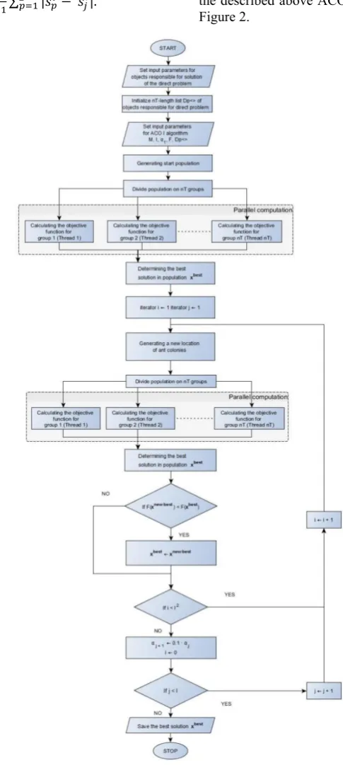
The control block diagram of the procedure serving for the reconstruction of heat flux q by using the described above ACO algorithm I is presented in Figure 1.
Ant Colony Optimization algorithm II
Now we describe the other version of ACO algorithm, presented also in [11]. The inspiration for developing this algorithm was also taken from the natural behavior of the swarm of ants. In this case, the solutions are considered as the pheromone spots. At the beginning, they are distributed randomly in the considered area. Next, the pheromone spots (solutions) are ranked in dependence on their quality and then to each pheromone spot the probability (corresponding to its quality) is assigned. The better is the solution, the higher is its probability of selection. In this way, we create the archive of solutions. In each iteration, M ants construct M new solutions (new pheromone spots) by using the probability density function (for example, the Gaussian function). Then the archive of solutions is updated by ranking the new and old solutions and by rejecting the M worst solutions. And similarly as in case of the ACO algorithm I, the ACO II was also adapted to parallel computing.
In order to describe this algorithm in details, we assume the following symbols: F − minimized function, x = (x1, ..., xn) ∈ D, nT − number of threads,
M = nT · p − number of ants in one population, I −number of iterations, L – number of pheromone spots, q, ξ – parameters of algorithm
Steps of the ACO algorithm II are as follows. Initialization of the algorithm
1. Setting parameters of the algorithm nT, L, M, I, q and ξ.
2. Generating L pheromone spots (solutions) and creating the initial archive T0.
3. Computing the values of minimized function for every pheromone spot and ranking the elements in T0, according to their qualities (from the best one to the worst one).
Iterative process
4. Assigning the probabilities to the pheromone spots according to the formula
𝑝𝑙= 𝜔𝑙
∑𝐿𝑙=1𝜔𝑙 𝑙 = 1,2, … , 𝐿,
𝜔𝑙= 1 𝑞𝐿√2𝜋𝑒
−(𝑙−1)2 2𝑞2𝐿2.
5. The ant chooses the l-th solution according to probabilities pl.
6. The ant transforms the j-th (j=1,2, … , n) coordinate of the l-th solution sjl by sampling the neighborhood by using the probability density function (Gaussian function):
𝑔(𝑥, 𝜇, 𝜎) = 1
𝜎√2𝜋𝑒 −(𝑥−𝜇)2
2𝜎2 ,
where 𝜇 = 𝑠𝑗𝑙, 𝜎 = 𝜉
𝐿−1∑ |𝑠𝑝 𝑙 − 𝑠
𝑗𝑙| 𝐿
𝑝=1 .
7. Steps 5-6 are repeated for each ant. Hence, we obtain M new solutions (pheromone spots). 8. Dividing the population on nT groups (groups will
be calculated in parallel way).
9. Determinating the value of minimized function for each new solution in population (parallel calculation).
10.Updating the archive Ti. 11.Steps 4-9 are repeated I times.
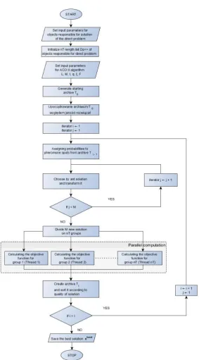
The control block diagram of the procedure serving for the reconstruction of heat flux q by using the described above ACO algorithm II is presented in Figure 2.
Figure 2. Control block diagram of the procedure reconstructing the boundary condition by using ACO II
4. Experimental results
Proposed algorithm were implemented in program C# 5.0 on computer with the following parameters: CPU: Intel Core i5-3230M 2.60GHz; OS: Microsoft Windows 10 Home; RAM: 8.00 GB. Multithreaded calculations were performed by using the Task Parallel Library.
We consider eqs. (1)-(4) with the following data *
500 [ ], 1[ ], 2 [ / ],
t s L m c J kg K
3
2 [kg m/ ],
2 [W m K/ ], u0 [ ],K( ) 0 [ ], 0.5
f x K
2
45 7
( ) 1400 exp ln [ / ].
455 4
t
h t W m K
The ACO algorithm I was executed for parameters nT = 4, M = 12, I = 3, α1 = 1,
whereas the ACO algorithm II was executed for parameters
nT = 4, M = 12, L = 8, I = 20.
of ACO algorithm I this number was equal to 336 and in case of ACO II algorithm it was equal to 252.
Function q is sought in the following form
𝑞(𝑡) = {
𝑎1, 𝑡 ∈ [0, 𝑡1),
𝑎2, 𝑡 ∈ [𝑡1, 𝑡2),
𝑎3, 𝑡 ∈ [𝑡2, 𝑡∗).
Exact values of a1, a2, a3 are known and are equal
to 200, 800 and 1300, respectively.
Inverse problem consists in reconstruction of the values of coefficients a1, a2 and a3 basing on the
measurement data (input data) 𝑈̂𝑖𝑗. The grid used to generate these data was of the size 300 × 5000.
We assume only one measurement point xp = 0.1
(N1 = 1) and the measurements from this point were
read in three courses, at every 0.5, 1, 2s (N2 = 1000,
500, 250). In order to investigate the impact of the measurement error on the quality of reconstruction and the stability of procedures, we perturbed the input data by the pseudorandom error of 1, 2 and 5% sizes.
In the process of minimizing functional (8), the direct problem must be solved many times. The grid used to solve the direct problem was of the size 100×1000. Let us notice that it is a different density than the the density of the grid used to generate the input data.
To determine the minimum of functional (8) the ACO I and ACO II algorithms were used. Both are the heuristic algorithms, therefore it is required to repeat the calculations a certain number of times. In this paper, we repeated the calculations ten times for each case and the ant population counted twelve individuals (M = 12). In order to make the procedures more quick working, and therefore more efficient, the ACO algorithms were adapted for parallel (multi-threaded) computations.
Tables 1, 2, 3 present the obtained reconstructions of coefficients a1, a2, a3 in dependence on the size of
input data disturbance at the measurement point xp = 0.1.
The results of reconstruction for both algorithms are very similar. As we can see by analyzing the tables, the coefficients ai (i = 1, 2, 3) are reconstructed
very well in all cases. In each considered case, the relative error of the coefficient restorations does not exceed 0.45%.
Figure 3 and 4 show the comparative convergence graphs of algorithms ACO I and ACO II in case of the measurements taken at every 1s. It appears that the ACO algorithm I converges slightly faster than the ACO algorithm II, however the slightly smaller value of minimized functional is obtained for the ACO algorithm II.
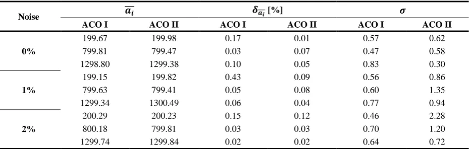
Table 1. Results of computation in case of measurements at every 0.5s in measurement point xp = 0.1 (𝑎𝑖- reconstructed value of
𝑎𝑖, 𝛿𝑎𝑖 - percentage relative error of 𝑎𝑖 reconstruction, 𝜎 - standard deviation of results (i=1,2,3))
Noise 𝒂𝒊 𝜹𝒂𝒊 [%] 𝝈
ACO I ACO II ACO I ACO II ACO I ACO II
0%
199.67 199.98 0.17 0.01 0.57 0.62
799.81 799.47 0.03 0.07 0.47 0.58
1298.80 1299.38 0.10 0.05 0.83 0.30
1%
199.15 199.82 0.43 0.09 0.56 0.86
799.63 799.41 0.05 0.08 0.60 1.35
1299.34 1300.49 0.06 0.04 0.77 0.94
2%
200.29 200.23 0.15 0.12 0.46 2.28
800.18 799.81 0.03 0.03 0.70 1.20
1299.74 1299.84 0.02 0.02 0.64 0.72
Table 2. Results of computation in case of measurements at every 1s in measurement point xp = 0.1 (𝑎𝑖- reconstructed value of
𝑎𝑖, 𝛿𝑎𝑖 - percentage relative error of 𝑎𝑖 reconstruction, 𝜎 - standard deviation of results (i=1,2,3))
Noise 𝒂𝒊 𝜹𝒂𝒊 [%] 𝝈
ACO I ACO II ACO I ACO II ACO I ACO II
0%
199.75 199.85 0.13 0.08 0.20 0.64
800.01 799.47 0.01 0.07 0.59 0.62
1299.17 1299.58 0.07 0.04 0.57 0.88
1%
199.78 199.72 0.11 0.14 0.36 1.19
799.26 799.10 0.10 0.12 0.41 1.50
1300.05 1298.98 0.01 0.08 0.80 0.97
2%
200.06 200.08 0.03 0.04 0.45 1.64
799.58 799.56 0.06 0.06 0.41 1.37
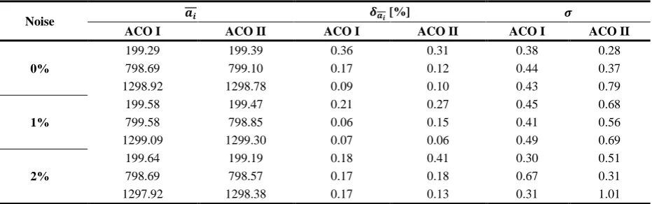
Table 3. Results of computation in case of measurements at every 2s in measurement point xp = 0.1 (𝑎𝑖- reconstructed value of
𝑎𝑖, 𝛿𝑎𝑖 - percentage relative error of 𝑎𝑖 reconstruction, 𝜎 - standard deviation of results (i=1,2,3))
Noise 𝒂𝒊 𝜹𝒂𝒊 [%] 𝝈
ACO I ACO II ACO I ACO II ACO I ACO II
0%
199.29 199.39 0.36 0.31 0.38 0.28
798.69 799.10 0.17 0.12 0.44 0.37
1298.92 1298.78 0.09 0.10 0.43 0.79
1%
199.58 199.47 0.21 0.27 0.45 0.68
799.58 798.85 0.06 0.15 0.41 0.56
1299.09 1299.30 0.07 0.06 0.49 0.69
2%
199.64 199.19 0.18 0.41 0.30 0.51
798.69 798.57 0.17 0.18 0.67 0.31
1297.92 1298.38 0.17 0.13 0.31 1.01
Figure 3 and 4 show the comparative convergence graphs of algorithms ACO I and ACO II in case of the measurements taken at every 1s. It appears that the ACO algorithm I converges slightly faster than the ACO algorithm II, however the slightly smaller value of minimized functional is obtained for the ACO algorithm II.
One of the main indicators for evaluating the results of the temperature reconstructio are the errors in measurement point xp = 0.1. Tables 4 and 5 show
the errors of temperature reconstruction in the control point for measurements read at every 0.5, 1 and 2s. Hence we can say that, in case of both algorithms, the temperature at the measurement point is reconstructed
very well. In most discussed cases, the slightly better results are obtained for ACO II, despite of the smaller number of executions of the objective function. The maximum relative error of the temperature reconstruction in each investigated case does not exceed 0.43% for ACO algorithm I and 0.41% for ACO algorithm II.
Figures 5 and 6 present the relative errors of reconstructing function q, occurring in the boundary condition, for the measurements taken at every 0.5, 1and 2s. In each considered case the relative error of function q restoration is lower than 0.72%. The worst results we obtained for the measurements read at every 2 seconds, that is for the most rare input data.
Figure 3. Comparative convergence graphs of ACO I (red dots) and ACO II (black dots) for measurements at every 1s, 0% perturbed input data (left figure) and 1% perturbed input data (right figure)
Table 4. Errors of temperature reconstruction in measurement point xp = 0.1 for measurements at every 0.5 and 1s (∆𝑎𝑣 - average absolute error, ∆𝑚𝑎𝑥 - maximal absolute error, 𝛿𝑎𝑣 - average relative error, 𝛿𝑚𝑎𝑥 - maximal average error)
ACO I
Noise 0% 1% 2% 0% 1% 2%
0.5s 1s
[ ] av K
0.1913 0.2696 0.1023 0.1130 0.1673 0.0830
max[ ]K
0.5206 0.3719 0.1269 0.3590 0.3254 0.1835
[%] av
0.0940 0.2000 0.0711 0.0816 0.0123 0.0330
max[%]
0.1651 0.4251 0.1451 0.1251 0.1101 0.0524
ACO II
Noise 0% 1% 2% 0% 1% 2%
0.5s 1s
[ ]
av K
0.1478 0.1701 0.0843 0.1541 0.2916 0.1300
max[ ]K
0.2720 0.2588 0.1007 0.2324 0.4483 0.2106
[%] av
0.0400 0.0724 0.0576 0.0633 0.1170 0.0452
max[%]
0.0662 0.1000 0.1151 0.0751 0.1401 0.0548
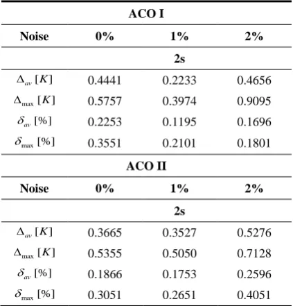
Table 5. Errors of temperature reconstruction in measurement point xp = 0.1 for measurements at every 2s
(∆𝑎𝑣 - average absolute error, ∆𝑚𝑎𝑥 - maximal absolute error, 𝛿𝑎𝑣 - average relative error, 𝛿𝑚𝑎𝑥 - maximal average error)
ACO I
Noise 0% 1% 2%
2s
[ ]
av K
0.4441 0.2233 0.4656
max[K]
0.5757 0.3974 0.9095
[%] av
0.2253 0.1195 0.1696
max[%]
0.3551 0.2101 0.1801
ACO II
Noise 0% 1% 2%
2s
[ ]
av K
0.3665 0.3527 0.5276
max[K]
0.5355 0.5050 0.7128
[%] av
0.1866 0.1753 0.2596
max[%]
0.3051 0.2651 0.4051
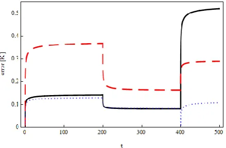
In Figure 7 and 8 we can see the distributions of the temperature reconstruction errors in the control point xp = 0.1 in case of measurements read at every
0.5s.
We can observe that the error of temperature reconstruction slightly decreases comparing the results obtained for the exact input data and the 1% perturbed input data, but then it increases comparing the results obtained for 1% and 2% perturbed input data. These differences however are minimal and they are prob-ably coused by the probabilistic nature of the used algorithms. In case of the perturbed input data we additionally deal with the disorder randomness. The
recobstruction errors of the results obtained with the aid of ACO algorithm II are a little bit smaller than the ones obtained with the aid of ACO I algorithm.
Figure 5. Relative errors of function q reconstruction obtained for various perturbations of input data and
for measurements at every 0.5, 1 and 2s (ACO I)
Figure 6. Relative errors of function q reconstruction obtained for various perturbations of input data and for measurements at every 0.5, 1 and 2s (ACO II)
Table 6 presents the times of single execution of each algorithm in dependence on the different number of threads. We terminated our research with four threads, since the usage of more than four threads resulted still in decreasing computation time, but it was not linear nor significant decrease. It may be noticed that the computation time of ACO II is smaller than the computation time of ACO I. This is due to the smaller number of executions of the minimized function needed by the second algorithm.
Figure 7. Distribution of the temperature reconstruction errors in measurement point xp = 0.1 for measurements
at every 0.5s and for various perturbations of input data (0% – solid line, 1% – dashed line, 2% – dotted line)
(ACO I)
Figure 8. Distribution of the temperature reconstruction errors in measurement point xp = 0.1 for
measurements at every 0.5s and for various perturbations of input data (0% – solid line, 1% – dashed line, 2% – dotted line) (ACO II)
Table 6. Times of single execution of the algorithms in dependence on the number of threads
number of threads
time [s]
ACO I ACO II
1 2394 1734
2 1388 1037
4 731 645
5. Conclusions
In this paper we considered the inverse problem for the heat conduction equation of fractional order. Goal of the inverse problem lied in the reconstruction of the second kind boundary condition. The direct problem was solved by using the implicit finite difference method and to minimize the proper functional two different Ant Colony Optimization algorithms (ACO I and ACO II) were used. In both cases, the obtained results were very good, by using these two algorithms we have received the satisfactory approximate solution.
The function q, defining the boundary condition of the second kind, was reconstructed very well. The reconstruction errors did not exceed 0.75% and did not exceed the input errors. The relative errors of temperature reconstruction in the measurement point were minimal and did not exceed 0.43%. We obtained slightly better reconstructions of temperature in results obtained by applying the ACO algorithm II.
It is worth to mention that the used algorithms can be easily adapted to parallel computing which reduces significantly the computation time. Executing the algorithm for 4 threads made the computations about three times faster than without multithreaded approach. Computation time of the second algorithm was smaller due to the smaller number of executions of the minimized function, but the results were very similar.
As the future work the authors plan to apply the artificial intelligence algorithms for solving the inverse problems of fractional order, for example in case of the 2D fractional heat conduction equation and/or the 3D fractional heat conduction equation. We also intend to verify the developed procedures by executing the numerical experiment on the basis of data obtained from real measurements taken of real objects.
Acknowledgement
We would like to express our thanks to all the Referees for the dedicated time and valuable remarks enabling to improve our paper.
References
[1] M. Ardakani, M. Khodadad. Identification of ther-mal conductivity and the shape of an inclusion using the boundary elements method and the particle swarm optimization algorithm. Inverse Probl. Sci. Eng., 2009, Vol. 17, 855–870.
[2] J. L. Battaglia, O. Cois, L. Puigsegur, A. Oustaloup. Solving an inverse heat conduction problem using a non-integer identified model. Int. J. Heat Mass Trans-fer, 2001, Vol. 44, 2671–2680.
[4] R. Brociek, D. Słota. Reconstruction of the boundary condition for the heat conduction equation of fractional order. Thermal Science, 2015, Vol. 19, 35–42 [5] R. Brociek, D. Słota, R. Wituła. Reconstruction of
the thermal conductivity coefficient in the time fractional diffusion equation. In: K. Latawiec, M. Łukaniszyn, R. Stanisławski (eds.), Advances in Modelling and Control of Non-integer-Order Systems, Vol. 320 of Lecture Notes in Electrical Engineering, Springer, 2015, pp. 239–247.
[6] R. Caponetto, G. Dongola, I. Fortuna, I. Petras. Fractional Order Systems. Modeling and Control Applications, World Scientific Series on Nonlinear Science, Series A, 2010, Vol. 72, World Scientific Publishing.
[7] A. Carpinteri, F. Mainardi. Fractal and Fractional Calculus in Continuum Mechanics. Springer, New York, 1997.
[8] A. R. Carvalho, H. F. D. C. Velho, S. Stephany, R. P. Souto, J. C. B. S. Sandri. Fuzzy ant colony opti-mization for estimating chlorophyll concentration pro-file in offshore sea water. Inverse Probl. Sci. Eng., 2008, Vol. 16, 705–715.
[9] S. Das. Functional fractional calculus for system iden-tification and controls. Springer, Berlin, 2008. [10] M. Dorigo, T. Stützle. Ant Colony Optimization. MIT
Press, Cambridge, 2004.
[11] M. Dorigo, C. Blum. Ant colony optimization theory: a survey. Theor. Comput. Sci., 2005, Vol. 344, 243–278.
[12] E. Hetmaniok, I. Nowak, D. Słota, A. Zielonka. Determination of optimal parameters for the immune algorithm used for solving inverse heat conduction problems with and without a phase change. Numer. Heat Transfer, 2012, Vol. B 62, 462–478.
[13] E. Hetmaniok, D. Słota, A. Zielonka. Experimental verification of immune recruitment mechanism and clonal selection algorithm applied for solving the inverse problems of pure metal solidification. Int. Comm. Heat & Mass Transf., 2013, Vol. 47, 7–14. [14] E. Hetmaniok, D. Słota, A. Zielonka. Experimental
verification of selected artificial intelligence algo-rithms used for solving the inverse Stefan problem. Numer. Heat Transfer, 2014, Vol. B 66, 343–359. [15] E. Hetmaniok, D. Słota, A. Zielonka. Using the
swarm intelligence algorithms in solution of the two-dimensional inverse Stefan problem. Comput. Math. Appl., 2015, Vol. 69, 347–361.
[16] D. Karaboga, B. Basturk. A powerful and efficient algorithm for numerical function optimization: artifi-cial bee colony (ABC) algorithm. J. Global Optim., 2007, Vol. 39, 459–471.
[17] D. Karaboga, B. Basturk. On the performance of arti-ficial bee colony (ABC) algorithm. Appl. Soft Compu-ting, 2008, Vol. 8, Issue 1, 687–697.
[18] D. Karaboga, B. Akay. A comparative study of artifi-cial bee colony algorithm. Appl. Math. Comput., 2009, Vol. 214, 108–132.
[19] J. Klafter, S. Lim, R. Metzler. Fractional dynamics. Resent advances, World Scientific, New Jersey, 2012. [20] J. Liu, M. Yamamoto. A backward problem for the
time-fractional diffusion equation. Appl. Anal., 2010, Vol. 89, 1769–1788.
[21] I. Martisius, D. Birvinskas, R. Damaševičius, V. Jusas. EEG dataset reduction and classification using wave atom transform. Lecture Notes in
Computer Science - ICANN'2013, Vol. 8131, 2013, 208–215.
[22] W. Mitkowski, J. Kacprzyk, J. Baranowski. Advan-ces in the Theory and Applications of Non-Integer Order Systems. Springer Inter. Publ., Cham, 2013. [23] W. Mitkowski, P. Skruch. Fractional-order models of
the supercapacitors in the form of RC ladder networks. Bulletin of the Polish Academy of Sciences Technical Sciences, 2013, Vol. 61, 581–587.
[24] D. Murio. Time fractional IHCP with Caputo fractio-nal derivatives. Comput. Math. Appl., 2008, Vol. 56, No. 9, 2371–2381.
[25] D. Murio. Stable numerical solution of a fractional-diffusion inverse heat conduction problem. Comput. Math. Appl., 2007, Vol. 53, No.10, 1492–1501. [26] D. Murio. Implicit finite difference approximation for
time fractional diffusion equations. Comput. Math. Appl., 2008, Vol. 56, No. 4, 1138–1145.
[27] A. Obrączka, J. Kowalski. Modelowanie rozkładu ciepła w materiałach ceramicznych przy użyciu równań różniczkowych niecałkowitego rzędu. In: M. Szczygieł (Ed.), Materiały XV Jubileuszowego Sympozjum „Podstawowe Problemy Energoelektro-niki, Elektromechaniki i Mechatroniki”, PPEEm 2012, Vol. 32 of Archiwum Konferencji PTETiS, Komitet Organizacyjny Sympozjum PPEE i Seminarium BSE, 2012, pp. 133–132.
[28] A. Obraczka, W. Mitkowski. The comparison of pa-rameter identification methods for fractional partial differential equation. Solid State Phenomena, 2014, Vol. 210, 265–270.
[29] K. Oprzędkiewicz. Approximation method for a frac-tional order transfer function with zero and pole. Archives of Control Sciences, 2014, Vol. 24, 409–425. [30] L. Özbakir, A. Baykasoglu, P. Tapkan. Bees algo-rithm for generalized assignment problem. Appl. Math. Comput., 2010, Vol. 215, 3782–3795.
[31] I. Podlubny. Fractional Differential Equations. Acade-mic Press, San Diego, 1999.
[32] A. F. Santos, H. F. Velho Campos, E. F. P. Luz, S. R. Freitas, G. Grell, M. A. Gan. Firefly optimiza-tion to determine the precipitaoptimiza-tion field on South Ame-rica. Inverse Probl. Sci. Eng., 2013, Vol. 21, 451–466. [33] K. Socha, M. Dorigo. Ant Colony Optimization in
Continuous Domains. Europan Journal of Operational Research, 2008, Vol. 185, No. 3, 1155–1173.
[34] M. D. Toksari. Ant Colony Optimization for Finding the Global Minimum. Appl. Math. Comput., 2006, Vol. 176, Issue 1, 308–316.
[35] J. G. Wang, Y. B. Zhou, T. Wei. A posteriori regula-rization parameter choice rule for the quasi-boundary value method for the backward timefractional diffusion problem. Appl. Math. Lett., 2013, Vol. 26, 741–747. [36] M. Woźniak. On Applying Cuckoo Search Algorithm
to Positioning GI/M/1/N Finite-buffer Queue with a Single Vacation Policy. In: Proceedings of the 12th Mexican International Conference on Artificial Intelligence – MICAI 2013, IEEE, 24-30 November, Mexico City, Mexico 2013, pp. 59–64.
[38] M. Woźniak, D. Połap. On some aspects of genetic and evolutionary methods for optimization purposes. Int. J. Electronics and Telecommunication, 2015, Vol. 61, No. 1, 7–16.
[39] M. Woźniak, D. Połap, C. Napoli, E. Tramontana. Real time cloud-based game management system via Cuckoo Search Algorithm. Int. J. Electronics and Telecommunication, 2015, Vol. 61, No. 4, 333-338. [40] M. Woźniak, D. Połap, C. Napoli, E. Tramontana,
R. Damaševičius. Is the colony of ants able to recogni-ze graphic objects? Communications in Computer and Information Science, 2015, Vol. 538, 376-387.
[41] L. Yan, F. Yang. Efficient Kansa-type MFS algorithm for time-fractional inverse diffusion problems. Comput. Math. Appl., 2014, Vol. 67, No. 8, 1507– 1520.
[42] G. Zheng, T. Wei. A new regularization method for the time fractional inverse advection-dispersion problem. SIAM J. Numer. Anal., 2011, Vol. 49, 1972–1990.
[43] Q. Zhuang, B. Yu, X. Jiang. An inverse problem of parameter estimation for time-fractional heat con-duction in a composite medium using carbon–carbon experimental data. Physica B, 2015, Vol. 456, 9–15.