A Time Step Energy Process Model for Germany - Model Structure and Results

EnergySludies Review Vol. 14. No. I. 2006 pp.35-57

A Time Step Energy Process Model

for Germany - Model Structure

and Results

DAG MARTINSEN, VOLKER KREY,

PETER MARKEWITZ and

STEFAN VOGELE

ABSTRACT

The new IKARUS-Model is a time-step dynamical bottom-up linear optimization model where each time interval is optimized by itself using the heritage from all periods before. Contrary to perfect-foresight models, this model does not take into account future changes in each time-step optimization. It therefore shows a more realistic character of prognosis and projection. Aspects like reaction on sudden changes (e.g. of energy prices), flexibility of technical scenarios, lost opportunities etc. can be examined. Interactions with macroeconomic I/O-models or dependencies on elasticities, technological learning etc. are possible. Recent calculations for Germany up to 2030 show that consistent and plausible future energy scenarios can be produced and analyzed.

36 Energy Studies Revieu: Vol. 14,Alo. 1

THE IKARUS PROJECT

At the beginning of the nineties, the fonner Gennan Federal Ministry for

Education, Science, Research and Technology (BMFT) initiated the

lKARUS-Project' with the objective to establish a sufficiently homogeneous database as well as models on which basis consistent energy scenarios and greenhouse gas reduction strategies could be fonnulated and calculated (Martinsen, Markewitz, Milller, Viigele and Hake, 2003). With the aid of the models, such scenarios and strategies can be developed and evaluated within the framework of energy technology and energy policy.

The lKARUS instruments consist of several models and a database developed for the area of the Federal Republic of Germany. The database is available as an infoTI11ation system, where the major section includes detailed technology data and furthermore extensive general data such as inventory, structure and scenario data with respect to energy economy and macro economy. From this database, model data is aggregated and tailored to the requirements of the lKARUS models. Energy models of the lKARUS instruments are:

• A classical bottom-up energy optimization model (LP-model, LP~

Linear Programming) describing the energy system on a national level.

• A very detailed space heat simulation model for different individual building types as well as for a partial or an entire building stock.

• A transport simulation model for passenger and freight transport

where energy consumption, costs and emissions are broken down to travel purposes and specific vehicles.

• A macroeconomic model including a demand-driven, dynamic

input-output model (10 model) with 24 sectors including nine

energy sectors. The model includes sectoral autonomous energy efficiency improvement (AEEI) factors to describe technical

progress as well as CES (Constant Elasticity Substitution)

production functions to represent substitution processes.

A review of the lKARUS models as compared with similar models world wide can be found in (Drake, Herzog, Kendall and Levin, 1997).

Martinsen. Krey. MarkeJ,j:itz&V6gele 37

LINEAR OPTIMIZATION MODEL

The linear optimization model is a central part of the IKARUS-instruments. In the following, model structure and some model results will be presented.

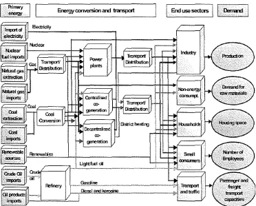
The model is mapping the energy system of the Federal Republic of Germany in the form of cross-linked processes (Figure I). A large number of technological options are included with their corresponding specific emissions and costs as well as possible networks of the energy fluxes. In addition, general political set-ups are considered (for example the agreement of the phase-out of nuclear power in Germany). The energy system is formed within the model in such a way that the demand for energy services is fulfilled. (Partial equilibrium model)

38 Energy Studies RevieVi-' Vol. 14. No.1

The model is structured into ten major sectors (primary energy,

electricity, district heat, refinery, gas, coal conversion, industry,

transportation, small consumer, household), where each sector is subdivided into subsectors. Thus, for example, the household sector is subdivided into single and multiple family houses and a further differentiation is made between old «1995) and new(>1995) buildings.

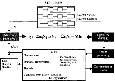
Both structural as well as numerical data, related to technologies, economy, energy policy and scenario data, are stored in a model database (MS Access). The system of equations to be solved is generated by bringing these two categories of data together as shown in Figure 2. In these equations gi is the name of restriction i, Xi the name of the variable j, aij the coefficient for variable Xi, bi the lower limit of the right hand side, Ci the cost-coefficient of variable X, in the objective function. The structural data contains about 3000 variables (energy converters, technical measures, imports of energy carriers etc.) and about 2000 equations (balances of energy-carriers, emissions, costs or load curves etc.). The numeric data are made up of general data, data for components of demand vectors, prices of imported energy carriers, upper and lower limits (bounds) of different categories and of COurse all technical data like specific costs, emissions, input and output of energy earners.

Figure 2. Calculation scheme for the IKARUS LP-model

STRUCTURE

Ca.3OO0 Variables Ca. 2000 Equations

~

~

Technical data (Costs, Emissions, Energy carriers)

a, b,c

User-changes

(Logfile)

DATA

General data

Demand, Importprices

Bounds

lvlartinsell, Krey. Alfarkewitz&V6ge/e 39

Before numeric and structural data are combined in a matrix generator, the model users can define their own scenario (e.g. energy prices, technological or political bounds etc.) and if desirable, make their own selection of technologies as well as changing any specific technical and economic attribute (for example efficiency, specific costs etc.). In addition to these changes, the user can add their own equations to the matrix or alter any existent user equation. Normally total system costs are chosen as the objective function (least costs).

The matrix generator will build up the linear equation system in the format of a standard MPS-file that is the input to a commercially available

mathematical optimizer (MOPS = Mathematical Optimization System) (Suhl,

1994). The result processing program will immediately calculate typical table values for energy, emission and cost balances and store these values in the model database. The presentation of user selected results in a tabulated or graphical form is made from a separate program where also multiple varying cases or scenarios can be compared to different levels of detail.

The new IK..A.RUS LP-Model is a time-step dynamical linear

4() Energy Swdies Review Vol. 14,No.1

like GREEN (Bumiaux, Martin, Nicoletti and Martins, 1992) or DART (Springer 1998) where it is referred to as recursive-dynamic or static expectations approach, but it is also used in bottom-up (i.e. technical) models like SAGE (EIA, 2003). A backcasting experiment comparing both the time-step and the perfect-foresight approaches with the help of a computable general equilibrium model can be found in a publication of Manne and Richels (Manne and Richels, 1992). A broader overview over different energy-economic modelling approaches can be found in the IPCC Third Assessment Report on Mitigation (Markandya, Halsnaes, Lanza, Matsuoka, Maya, Pan, Shogren, de Motta, Zhang and Taylor, 200 1).

In addition, interaction with macroeconomic input-output models or dependencies on elasticities, technological learning, economy of scale etc. as well as other non-linear (dynamical) effects can be taken into account. A major part of these effects can probably be considered without an iterative optimization process if sufficiently short time-step intervals are chosen. At the moment, some of these non-linear aspects are handled in a semi-manual way. A real dynamic recursive model concept will be prepared in the time to come. In order to compare results from the time-step approach with results from a perfect foresight model, we also operate a multiple period MARKAL (Fishbone, Giesen, Goldstein, Hymmen, Stocks, Vos, Wilde, Zecher, Balzer and Abilock, 1983) based optimization model having a comparable structure and using the same IKARUS data. The MARKAL model is a stand-alone application and not a member of the IKARUS instruments itself (Kraft 1997). Itis an often used model for Gemlan energy scenarios.

Martinsen. Krey. Markewitz& Vogele 4J

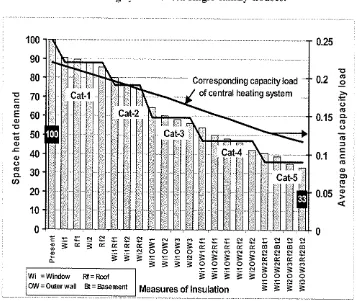
Figure 3: Space-heat demand for different measures of thermal insulation and corresponding annual capacity load of the central heating system in old single-family-houses.

0.25

"0

0.2

11

~_<.>

m

m +0.15

g-<.> m

'"

SO! ~ N

~ ~

"'

'"

'" '"

SO! SO! SO!

"

"

'" '" '" '"

0 0 N N M M

'"

_{" " "}

_"

" "

;::

;:: ;:: ;::

wft;t~·~·~m.;,m~_

..__

"

;::

_'"

"'

N M M

~

~

'"

_"

'"

_'"

'"

_"

_"

_"

'" '"

00 _{~ N}

0 0 0 0

~ N M

e

_{;:: ;::}

"

"

Q.

;::

"

;::

.-;::

Wi =Window Rf=Roof

" "

100 90 80 "0 ₇₀ c m E 60 Q) "0

-

_"

Q) .<: 40 Q) <.> m 30 a. C/) 20 10 0 SCENARIOS

The scenarios presented here serve as examples of energy projections for Germany achieved by the model. They are typical, but of course do not cover all plausible future developments. Before showing some typical results from the lKARUS LP-model runs for Germany up to 2030, we will describe some of the most important assumptions that are to be considered when evaluating the results.

42 Energy Srudies RevieVl! Vol. 14, No.1

Table 1: Demographic and overall economic data.

Unit Relevant numbers Annual chances in %/a

2000 2010 2020 2030 2000110 2010120 2020/30

Popuiation MiD. 81.99 81.50 80.34 77.98 -0.06 -0.14 -0.30

Number of households Mio. 37.5 38.5 38.80 38.10 0.26 008 -0.18 Persons per Household # 2.19 2.12 2.07 205 -032 -0.22 -0.12

~partments Mia. 3682 39.64 41.60 43.08 0.74 0.48 035

Apartments per

1000 Households # 982 1030 1072 1131 0.48 0.41 0.53

otal floor space Mia. m2 _{3116.5 3408.6 3637.1 3838.6 0.90 0.65 0.54} Floor space per Capita m' 38.0 41.8 45.3 49.2 0.96 080 084 Size of singie-famiiy house m2 _{105.95 10831 110.62 113.43 0.22 0.21 0.25}

Size of multi-familv house m' 65.94 66.45 66.88 67.35 0.08 0.06 0.07 Number of employed Mio. 37.54 37.34 37 34.92 -0.05 -0.09 -0.58

Gross domestic product 10'D(95) 1963.8 2366.7 2797.5 3189.6 1.88 1.69 1.32

GDP per Capita 23951 29039 34821 40903 1.94 1.83 1.62

Value added industry 10' : 36265 440.65 507.68 585.21 1.97 1.43 1.43

Due to the smaller number of children per family, a growing life

expectancy as well as a trend towards single person households, the number

of the private households will increase up to 2010. In the last decade,

however, this number will decrease again due to a declining total population. The number of apartments and houses climbs by far more strongly than the number of the households. The reason is the increasing number of second homes for working commuters as well as of pensioner households. Because of this, the number of apartments increases from 36.8 million today to about 43 million in the year 2030.

It is assumed, that the average apartment size in new single-family

houses will rise from 106 m' today to 113 m' in the year 2030. The size of an average apartment in multiple family houses changes only slightly from 66 to 68 m' during the model's time horizon. The total floor space increases by 23% up to the year 2030. As a result, the floor space per capita rises from today 38 m' to 49 m' in 2030.

lllfartinsen. KreJ:, JHarke.vilz& V6gele 43 chemistry is growing with about 1.6% per year, the growth rate of other energy intensive sectors like iron industry, cellulose and paper is by far lower. The number of employees in the small consumer sector increases slightly up to 2020. Thereafter, it drops noticeably giving in this sector about one million employees less in 2030 (30.4 millions) compared to 2000 (31.4 millions). At the same time, the private and public services gain importance while in particular the number of employees in agriculture and forestry shows a further decrease.

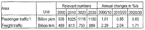
The transportation sector is divided into passenger transport and freight transport, as well as into long-distance and short-distance traffic. The demand for passenger transport is growing from 926 billion pkm (passenger kilometers) in the year 2000 to 1190 billion pkm in 2030 (Table 2). The increase of freight traffic, however, is much stronger. It climbs from 489 billion tkm (ton kilometers) to 889 billion tkm, i.e. an increase of more than 80% in the coming 30 years.

Table 2: Demand of passenger and freight traffic.

!'Irea Relevant numbers Annual chanaes in%/a

Unit _{2000 2010 2020 2030} 2000/10 2010120 2020130 Passenger traffic1) Billion pkm 926 1025 1116 1190 1.01 0.85 0.65 Freiqht traffic Biilion tkm 489 613 750 889 229 2.04 1.71

I)Without pedestrians and cyclists. Air traffic: Domestic concept

The prices for the most important imported energy carriers are assumed to have only a moderate increase over the coming 25 years (Hom, 2002).

44 Energy Sludies Review Vol. J4.No. J

Table 3: Some important bounds concerning energy policy and quantity potentials.

Unit 2000 2010 2020 2030

Domestic hard coal PJ 1005 > 300 -) -\

lmood of hard coal PJ 910 < 1800 < 2400 < 3000

1521 > 800 > 800 > 800

Extracfion of lignite PJ

< 1600 <1500 < 1400

Domestic natural gas PJ 633 < 700 < 600 < 500

lmooded nafurat Das A PJ 2683 < 4000 < 4000 <4000

~ednatural qas B PJ < 4000 < 4000 <4000

Wind power GW 5.9 > 12 > 12 > 12

Nuclear power plants GWnello 222 18.3 78 0

With regard to the future role of nuclear energy, the remaining residual capacities for the nuclear power plants were estimated based on the agreement between the Federal Government and the utilities concerning the nuclear phase-out. For wind power we assumed a future minimum capacity of 12 GW corresponding to the installed capacity at the end of 2002.

SCENARIO RESULTS

These assumptions lead to primary energy consumption as shown in Figure 4.

Even in this reference scenario, the primary energy consumption is declining. In the year 2030, it is about 15 % lower than in 2000. Beside final energy savings, this is mainly due to changes in the conversion sector. However, it is also partly caused by the energy balance sheet values of non-fossils. For example, the primary energy value of nuclear electricity is based on an efficiency of 0.33. The nuclear reactors are substituted (nuclear phase-out) by fossil power stations having a much higher efficiency. This leads to a calculated drop of primary energy. Up to 2030, the shares of coal+lignite and oil are decreasing, and the contribution of natural gas and renewables are

Increasmg.

In Germany there has been a continuous discussion in the last 10 - 15

l\1artinsen. Krey, Marken"itz&VogeJe 45 Figure 4: Projection of primary energy in the reference case.

Imposing various technical and economic guidelines in order to advance innovation and energy saving for example by law or subsidies.

16000

14539

14000

12000

10000

PJ 8000

6000

._---4000

2000 ~

-_

0

2000

Innovation+Saving:

2010 2020 2030

Reduction scenario: Giving boundary conditions only and leaving it to the energy system to decide which options should be chosen to fulfill these conditions.

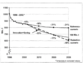
The energy related amount of CO, emissions in Germany caused by energy conversion in 2003 was about 837 million tons. This is a reduction of about 15% compared tothe emission level of 1990. Figure 5 shows the CO," emissions (temperature corrected values) in the reference case as well as for the reduction and innovation+saving scenarios. The high reduction rates in the first half of the nineties were in particular due to measures of restructuring in East Germany that among other things led to a drastic reduction of the use of

46 Energy Studies Review Vol.14,No.1

Figure 5: CO,-emissions in Germany.

1000 1990 _2002*

m "_ _"C=...;;:::;...

;;.:...:=.j

.

.-=_:1%,.__ ..

-=,

_~

•

.,;

::E

700

600

-21% -21%

Reference-scenario

500~-"----"--""-" m " "

-1990 2000 2010 2020 2030

corrected values

In the projection of the reference scenario, the CO2 emissions drop by

about 5% from 2000 to 2010, decrease a further 2 percent until 2020 and remain constant thereafter- This is close to the climate gas reduction obligation made for Germany within the framework of the EU-Burden sharing process, i_e_ -2 I % in 2010 when compared to 1990 including all climate gases (Commission of the European Communities, 2004), (Council of the European Union, 2002)_ More far-reaching reduction goals like a decline of 40 % up to the year 2020 or 2030, as currently discussed in energy policy, are clearly missed in the reference scenario_ Therefore, a reduction path with a linear CO, decrease is imposed to the model demanding a 40% reduction of CO, emissions in 2030 as compared to 1990:

• 2010: - 23% as compared to 1990

• 2020: - 31 % as compared to 1990

• 2030: - 40% as compared to 1990

Figure 5 also shows the resulting CO2-emissions from the

lv!arlinsen. Krey. /iI!arke"....ilz& Vi5gele 47

more close to a simulation where the most important assumptions divergent from the reference scenario are:

• Power stations: Improvement of efficiency by 2-3 percent points. • Industry: Measures of energy saving for production and utilization

of process heat and electricity.

• Small consumer: Insulation of buildings within cycles of renovation. Measures for saving of process heat and use of electricity.

• Household: Insulation of old buildings within cycles of renovation. Improved space heat standard. More efficient use of electricity in new appliances.

• Transport: Vehicles with a clear reduction of fuel consumption.

Share of public transport to modal split at the upper limit.

The corresponding CO2-emissions show a more hyperbolic curve

compared to the linear reduction scenario showing a -25% reduction in 2010 and ending up with a reduction of about -35% in 2030. The cumulated emissions for the period 2000 - 2030 are about the same in both scenarios.

In the following, we will limit ourselves to mainly describe deviations of the innovation+saving and the reduction scenario from the reference scenario. A detailed description of the reference scenario can be found in (Martinsen, Markewitz, Miiller, Vogele and Hake, 2003).

Figure 6 shows the share of sectors to the saving of final energy in the innovation+saving scenario as compared to the reference scenario. The main contributors to this saving are the household and transport sector. The relative saving in 2030 is 9% in the industry sector', about 16% in the sector of small consumers and reaches nearly 25% in both sectors household and transport. In total, the added innovationsin technology and measures of energy saving result in a reduction of 18% of the final energy demand as compared to the reference case in 2030. In the reduction scenario (not shown in figure 6), the saving of final energy is considerably smaller with a total of -8% in 2030.

2A considerable reductionof final energy in the industry (- 11%) has taken place between 2000

48 Energy Studies Reviel1' Vol. 14.1'/0.1

Figure 6: Share of sectors to the saviug of final energy in the

innovation+saving scenario.

1381 ~15%*

609

2030

o

.Irdustry

o

590

2020

799

~8%*

2010

1800

1600

1400

1200

1000

PJ

800

600

400

200

0

2000

The share of sectors is dominated by the household sector although far weaker (and less costly) measures of thermal insulation are taken as compared

to innovation+saving. In the transportation sector, additional

(non-autonomous) saving occurs only at the end of the time considered. In order to meet the CO, constraint, additional measures are taken in the conversion sector like very efficient natural gas combined cycle power plants substituting coal plants. Measures in the conversion sector are mostly cheaper than in the end use sectors.

Martin<;en. Krey. Markewitz&Vogele 49

household sector with a 22% decrease of CO2emissions in 2030 compared to

the reference scenario. However, the relative share of households to total reduction is dropping from 20% in 2010 to 11 % in 2030. A significant share of other end-use sectors (small consumer, industry, transport) does not show up until the last time period.

Figure 7: Share of sectors to CO2reduction in the reduction scenario.

Transport: -5,5% 12 Miot

Small consumer: -17,8% 9 Miot

-12,3% 12 Miot

Conversion: -41,9% 135Miot (Incl. Power-and heat station:

-- 124, Mio t)

2030

*Compared to reference scenario -i1":' Household: -21,9'Y~ 22 Miot

2020

-31% - 40% as compared to 1990

Mio.t

m ' " _ _, , _ , -23,9%

2010

-23%

108Mio. t

+

-220

200

180

160

140

-

120

0

::;;;

₁₀₀

80

60

40

20

0

2000

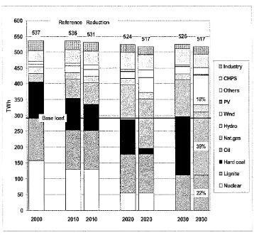
Because of the dominant part of the electricity sector to meet the CO2

constraint, we exemplarily show the structure and changes of the electricity production in the model results in figure 8 with the reference scenario (grey) to the left and the reduction scenario (black) to the right.

50 EnergySwdies Revinv Vol. 14, No. I

power plants which have a share of nearly 40% to total electricity production in 2030. Another significant difference between the reduction and the reference scenario is the strong increase of wind power reaching a capacity of 35 GW (onshore and offshore) in 2030 and corresponding to a share of 18% to the electricity production. Also the share of CHP based on biomass is increasing. In addition an overall modernization and increase of efficiency take place. Altogether, the CO, reduction is about 120 million tons in 2030 compared to the reference scenario.

Figure 8: Structure of electricity production in the reference and reduction scenario.

500

400

J:: 350

;;:

t-300

250

200

150

100

50

Reference Reduction

o Industry OCHPS

oOthers

I!lPV o Wind

oHydro

lJ Natgas

DOil

• Hard coal

illUgnite oNuclear

2000 2010 2010 2020 2020 2030 2030

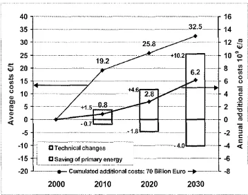
llt!artinsen. Krey, MarkelA."itz& Vogele 51 reduction and reference scenario. In the period 2000 to 2030 the costs cumulate to about 70 billion eufO. The corresponding average specific CO, reduction costs are ca. 19 Elton in 2010 and ca. 32 Elton in 2030.

Figure 9: Annual and specific costs of CO, reduction in the reduction

scenario. 40 35 30 25 ~ 20

""

-

0

<J

10

Ql

OJ

co_{~ 5} Ql >

°

«

. ..._.. ._. .__...__._~ .32.5.~_

-- - --+10.2r--'···~

6.2

'"-~~.._~, --~--_._-~~--~~

. -+1.5°.8 .

-0.7

DTechnical changes

D Saving of primary energy

.L._ __ . -Cumulated additional costs: 70 Billion Euro _..._ _.L 16

14

12

-

""

1

°

"'0

8 Ul

-

6 0<J

4 "iiic: .2 2

.

...

"0

°

-2

_"

c:

-4

«

-6

-8

2000

2010

2020

2030

The marginal costs are of course higher, being about 95 Elton in 2030. These costs have an exemplary character only. They depend on assumptions made and bounds set (tables I - 3) as well as on time dependency and magnitude of the CO, constraint. For example changing the restriction for CO2emissions in 2030 from -40% to -31 % (= 2020 value) respective -50%,

52 Energy Studies Review Vol. 14,No.1

ADDITIONAL POSSSIBILITIES OF TIME-STEP OPTIMIZATION

The results shown above do not differ very much from similar perfect foresight optimizations. The reason is the relatively smooth time dependency of assumptions and restrictions made for these calculations. However, in the perfect foresight calculations generally measures will be chosen earlier than in the time-step calcnlations to avoid a more costly action at a later time period.

A further use of the time step model will be the investigation of lost opportunities and the flexibility of technological scenarios to unexpected sudden changes as this will in general lead to additional information compared to the perfect foresight approach.

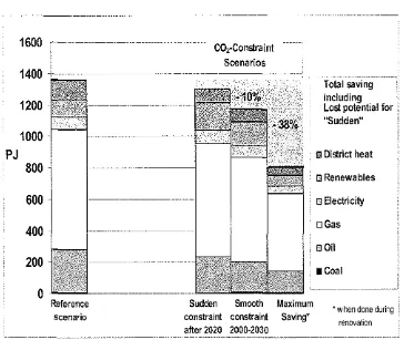
Figure 10: Demand and lost potential of space heat savings for old buildings in household 2030.

CO2·Constraint

Scenarios

IJ Bectricity I!IDistrict heat

-600

1200

1400

+ - - - -.. ----.---, .--.,,-.-.-,.... - ...,

"Sudden"

1000

PJ

400

Reference

scenario

Sudden

constraint

after 2020

Smooth

constraint

2000·2030

Maximum Saving*

!!lOil

• Coal

*when done during renovation

Iv!artinsen. Krey. !tIarke.vitz&V6gele 53

buildings to be renovated in one time period is limited. The figure illustrates the demand of space heat in 2030 for three CO,-scenarios, all constrained to a 40% reduction of CO, in 2030 as compared to 1990.

• "Sudden" constraint after 2020. In this scenario, there is no CO, constraint before 2020. Thereafter, however, a sharp decrease of CO, is imposed. The model, not knowing the future, will apply additional (to reference scenario) insulation measures only after 2020, not before. The potential of space heat savings due to insulation of buildings having their renovation in the period 2000 _. 2020 is therefore lost. (As far as the CO, constraint is concerned, this is partly compensated by the increased use of renewabIes).

• "Smooth" constraint 2000 - 2030. This scenario is identical to the reduction scenario as described above with a linear increase of the CO, restriction. The result of this scenario is close to a perfect foresight optimization and the model will choose insulation measures during renovation in all periods.

• "Maximum" saving. This case model will make use of the maximum potential of insulation measures with a high degree of space heat savings (category 5 in figure 3) within renovation at all

time periods.

• The potential of saving lost in the "Sudden" scenario as compared to the "Smooth" scenario is about 10% and therefore, comparatively small. However, in the "Sudden" scenario more expensive measures are taken in a short time compared to the "Smooth" scenario where several low to medium cost measures are chosen distributed over a longer time period.

• In comparison to the "Maximum" scenario, where a saving of space

heat of about 41% is achieved when compared to the reference

scenario, the lost potential is considerable: 38% for the "Sudden" and 31% for the "Smooth" scenario.

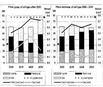
The dynamics of prices for energy carriers is another important aspect in a model without perfect foresight. An example of the result of a sudden change of prices for imported oil, oil-products and natural gas after 2020 as compared to a scenario with a steady increase of these prices from 2000 to 2030 is presented in figure II for the electricity sector.

54 Energv Studies Review Vol. 14,No. J

Figure 11: Installed capacity and load of lignite, hard coal and gas power plants for two price scenarios.

Price jump of oil+gas after 2020

0.0 0.2 0.1 0.5 0.4 0.3 0.6 2030 2020 70 60 50 40 30 20 10 0 2000 2010

Price increase of oil+gas 2000·2030

Annual

CJN ~d

80 ',--'."-.""'"."-_::--:.:-"'.'

':.:::.-.""'C...:-..

2030 2020 2010

Load • • • _ ";-";--;;'""-;"-;".;;"._"~ 0.8

i

I

~,

i

-i

i

I

I

o

Gas .. .. .. Load Ilgnite

--·Hard coal load~·'~,Gasload Lignite _ Hard coal

Gas .. .. .. Lignite load

-Hard coal load~~~,w,Gasload

Martinsen, Kre)", Mal'kel-vjtz&V6gele 55

The example above shows that also least cost scenarios that are based on a special course of energy prices can lead to an irreversible build-up of costly surplus capacities when unforeseeable price changes occur.

SUMMARY AND OUTLOOK

In the paper, a new version of the IKARUS energy systems optimization model for Germany was described. In contrast to former versions and also other models of the same type, it employs a myopic time-step optimization approach. Apart from the new methodology, the model structure along with the most important energy-economic assumptions have been outlined. Two scenarios for Germany until 2030 have been developed with the help of the model and the results of these calculations have been presented. Several model runs of the time step IKARUS model show that with this model consistent, reasonable and plausible future energy scenarios can be produced and analyzed. In addition, the time-step optimization approach enables the modeler to investigate the impact of sudden changes on the energy system. An abrupt introduction of CO2mitigation obligations and a sudden rise of oil and

natural gas prices served as examples for the application of the new methodology.

Another aspect of future work will be the endogenous integration of non-linear effects like for example learning curves. These, together with a more detailed vintage capacity calculation, will be components of an integrated dynamical recursive model structure.

The increasing entanglement of national economies and the liberalization of energy markets in the ED have a strong impact on the development of the member countries' energy systems. In particular the exchange of grid-bound energy carriers such as electricity and natural gas and the construction of the required infrastructure is even a primary target of the European Commission.

56 Energy SlUdies Review Vol. 14. No. I

REFERENCES

Burniaux, J.-M., J.P. Martin, G. Nicoletti, J.O. Maltins, (1992) 'GREEN: A Multi-Sector, Multi-Region General Equilibrium Model for Quantifying the Costs of Curbing C02 Emissions,' Working Paper 116, OECD, Paris.

Commission of the European Communities (2004) 'Catching Up with the Community's Kyoto Target,' COM(2004) 818, Brussels, 20.12.2004.

Council of the European Union (2002) 'Council Decision of 25 April 2002 concerning the approval, on behalf of the European Community, of the Kyoto

Protocol to the United Nations Framework Convention on Climate Change and

the joint fulfilment of commitments thereunder,' (2002/358/CE),Official Journal L(Legislation) 45: 130: 1-20.

Drake, E.M., HJ. Herzog, M. Kendall, J. Levin (1997) 'Energy Technology Availibilty: Review of Longer Term Scenarios for Development and Deployment of Climate-Friendly Technologies,' Prepared for The Intemational Energy

Agency, Paris.

EIA Office of Integrated Analysis and Forecasting (2003) 'Model Doeumentation Report: System for the Analysis of Global Energy Markets (SAGE),' DOE/EIA-M072(2003)/l, Energy Infomlation Administration, U.S. Department of Energy, Washington DC.

Fishbone, L.G., G. Giesen, G. Goldstein, H.A. Hymmen, KJ. Stocks, H. Vos, D. Wilde, R. Zocher, C. Balzer, H. Abiloek (1983) 'User's Guide for MARKAL,' Brookhaven National Laboratory and KFA JUlich.

Hom, M. (2002) 'Entwicklung der Importpreise fur fossile Energietriiger bis wm

Jahr 2030 [Development of Fossil Fuel Import Prices until 2030],' In lKARUS-Bericht Nr. 3-10, Forschungszentrum lillich.

Kraft, A. (1997) 'Einsatz der linearen Programmierung zur Analyse des energiewirtschaftliche Potentials von Brennstoffzellen [Application of Linear Programming for the Analysis of the energy-economic Potential for Fuel Cells],' Diploma thesis, Technical University of Aachen, Aachen.

Loulou, R., G. Goldstein, K. Noble (2004) 'Documentation for the MARKAL Family of Models,' lEA Energy Technology Systems Analysis Programme,

http://www.etsap.org/documentation.asp .

)\tfartinsen. Krey. Marke.-t'itz&Vogele 57

Martinsen, D., P. Markewitz, D. Mliller, S. Vogele and l-Fr. Hake (2003) 'IKARUS - Energieszenarien bis 2030 [IKARUS - Energy Scenarios until 2030],' In Das lKARUS-Projekt: Energietechnische Perspektiven fUr Deutschland, Schriften des

Forschungszentrums Ji.ilich, Reihe Umwelt/Environment, Band/Volume 39.

Messner, S., M. Strubegger (1995) 'User's Guide for MESSAGE III,' IIASA Working Paper WP-95-69, International Institute for Applied Systems Analysis,

Laxenburg, Austria.

Markandya, A., K. Halsnaes, A. Lanza, Y. Matsuoka, S. Maya, J. Pan, J. Shogren, R.S. de Motta, T. Zhang, T. Taylor (2001) 'Costing Methodologies' in Metz, B.,

O. Davidson, R. Swart, J. Pan (eds.) Climate Change 2001: Mitigation. Third

Assessment Report (~l the IPCC, Cambridge University Press. Cambridge,

http://www.grida.no/climate/ipcc tar/wg3/,pp. 455-498.

Springer, K. (1998) 'The DART General Equilibrium Model: A Technical Description,' Working Paper 883, lnstitut fUr Weltwirtschaft, Kiel.

Statistisches Bundesamt (2000) 'Bevolkerungsentwicklung Deutschlands bis zum Jahr 2050. Ergebnisse der 9. koordinierten Bevolkerungsvorausberechnung [Population Development in Germany until 2050. Results of the 9th Coordinated Projection],' Wiesbaden.