Reliable Robust Sampled-Data H∞ Output Tracking Control with Application to Flight Control

(1)

Reliable Robust Sampled-Data

H

∞

Output Tracking Control

with Application to Flight Control

Yueying Wang, Pingfang Zhou

1

, Quanbao Wang, Dengping Duan

School of Aeronautics and Astronautics, Shanghai Jiao Tong University, Shanghai 200240, China e-mail: 1_{[email protected]}

http://dx.doi.org/10.5755/j01.itc.43.2.4821

Abstract. This paper is concerned with the problem of robust H∞ output tracking control for uncertain

sampled-data systems with probabilistic actuator failures. By assuming that each actuator fault takes values randomly in a finite set, a new actuator-failure-mode is proposed. Lyapunov-Krasovskii functional combined with the input delay approach as well as the free-weighting matrix approach are employed to establish the H∞ performance, and the controller design

is cast into a convex optimization problem with linear matrix inequality (LMI) constraints. The designed reliable controller can guarantee that the output of the closed-loop sampled-data system tracks the reference signal without steady-state error. An airship model is considered in this paper and its simulation results are given.

Keywords: probabilistic actuator failures; output tracking; sampled-data control; convex polytope; flight control; parameter uncertainty.

1. Introduction

In the past years, output tracking control has received considerable attention due to its wide applications in dynamic processes in industry such as robot control [1], flight control [2-4] and motor control [5, 6]. The main objective of output tracking is to design a controller to guarantee the output of controlled system tracking the reference signal as close as possible, which is more general and more difficult than stabilization. Up to date, many results have been reported on output tracking [7-9].

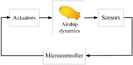
As is well known, with the fast development of microprocessor and electronic technologies, digital computers are widely used to control continuous-time systems in modern control systems. For example, in a flight control system about airship (see Figure 1), a microcontroller is usually used to sample and quantize a continuous-time measurement signal, and then produce a discrete-time control input signal, which can be further converted into a continuous-time control input signal using a zero-order holder. Such control systems involve both continuous-time and discrete-time signals in continuous-time framework are referred to as sampled-data systems. Considerable research efforts have been made on various aspects of sampled-data systems, such as control systems [10-12] and filtering problems [13-15]. It is worth mentioning that little progress has been made to design controllers for uncertain sampled-data systems to make the output

to track the reference signal without steady-state error, although it is of both theoretical significance and practical importance.

In reality, because of the actuators aging, zero shift and electromagnetic interference, actuator failures are unavoidable, which may lead to intolerable performance of the system. Therefore, it is necessary and important to design controllers that can tolerate actuator failures. A common assumption in most of the existing results on reliable control is that the actuator failure model is depicted as an unknown bounded constant [16-18]. It is not difficult to understand that in some situations, however, actuator failures may happen in a random way. Recent works assume that the actuator failures satisfy certain probabilistic distribution on the given intervals [19-21].

Motivated by above discussions, this paper focuses on the controller design for a class of uncertain sampled-data systems with probabilistic actuator failures. The main contributions of this paper are as follows:

1) This is the first paper that a controller is designed to make the output of uncertain sampled-data system to track the reference signal without steady-state error, and the results can be applied to flight control and other areas.

(2)

Figure 1. Architecture of airship control system

2. Problem formulation

Consider the following uncertain linear system:

{𝑥̇(𝑡) = 𝐴(𝜆)𝑥(𝑡) + 𝐵(𝜆)𝑢 (𝑡) + 𝐷(𝜆)𝑤(𝑡) 𝑦(𝑡) = 𝐶(𝜆)𝑥(𝑡) + 𝐷 (𝜆)𝜂(𝑡) (1) where 𝑥(𝑡) ∈ 𝑅 is the state vector, 𝑢 (𝑡) ∈ 𝑅 is the actuator output considering possible failure, 𝑦(𝑡) ∈ 𝑅 is the output, 𝑤(𝑡) ∈ 𝐿 [0, ∞) denotes the exogenous disturbance signal, 𝐴(𝜆), 𝐵(𝜆), 𝐷(𝜆), 𝐶(𝜆) and 𝐷 (𝜆) are system matrices containing uncertain parameters, represented by 𝜆 . Assume that Ω ≜ (𝐴(𝜆), 𝐵(𝜆), 𝐷(𝜆), 𝐶 (𝜆), 𝐷 (𝜆)) ∈ ℜ, where ℜ is a given convex-bounded polyhedral domain described by 𝑟 vertices

ℜ ≜ {Ω|Ω = ∑ 𝜆 Ω ;

∑ 𝜆 = 1,

𝜆 ≥ 0}(2)(2)

with Ω ≜ (𝐴, 𝐵, 𝐷, 𝐶 , 𝐷 ) ∈ ℜ denoting the vertices of the polytope.

In this paper, the following actuator failure model will be adopted:

𝑢 (𝑡) = Θ𝑢(𝑡) = ∑𝜃 Δ 𝑢(𝑡), (3)

where Θ = 𝑑𝑖𝑎𝑔{𝜃 , 𝜃 , … , 𝜃 }, 𝜃(𝑙 = 1, … , 𝑚) are 𝑚 unrelated random variables and

Δ = 𝑑𝑖𝑎𝑔 {0, … , 0⏟

, 1, 0, … , 0⏟

}.

It is assumed that 𝜃 takes values in a finite set, that is 𝜃 ∈ {𝜏 , 𝜏 , … , 𝜏 }. In addition, the process

{𝜃 } is assumed to be independent and

identicallydistributed, with the probabilities given by 𝑃𝑟𝑜𝑏{𝜃 = 𝜏 } = 𝛼 ,

𝑙 = 1, … , 𝑚, 𝑗 = 1, … , 𝑞 (4)

where 𝛼 is a positive scalar and ∑𝛼 = 1.

Remark 1. In the most of existing results on reliable control, variable 𝜃 is an unknown constant with known lower and upper bounds (see, for example [16–18]). Some other results, for example [19–21], assumed that the variable 𝜃 satisfies a certain probabilistic distribution on the given interval [0; 𝜃], which is more general and practical than the former results in some situations. In many real control

systems, however, the type of actuator failures is finite. In this situation, the assumption in (4) can better describe the failure characterization.

Remark 2. In this paper, the random variable 𝜃 takes values in a finite set. For 𝜃 = 0, it means complete failure of the 𝑖th actuator; for 𝜃 = 1, it means that the 𝑖th actuator is in good work condition; for 0 < 𝜃 < 1, it means partial failure of the 𝑖th actuator; for 𝜃 > 1, it means the actuator-amplifier with forward drift.

It is well known that the tracking error integral action of controller can effectively eliminate the steady-state tracking error. Similar to Ye and Yang [2], and Liao et al. [4], we introduce the following augmented system state-space description of system (1) with actuator failure model:

𝜍̇(𝑡) = 𝐴̅(𝜆)𝜍(𝑡) + 𝐵̅(𝜆) ∑ 𝜃

Δ 𝑢(𝑡)

+𝐷̅(𝜆)𝑤̅(𝑡) (5)

𝑧(𝑡) = 𝐶̅𝜍(𝑡), where

𝜍(𝑡) = [𝑥 (𝑡) (∫ 𝑒(𝑡)𝑑𝑡) ] ,

𝑒(𝑡) = 𝑟(𝑡) − 𝑆𝑦(𝑡),

𝑤̅(𝑡) = [𝑤 (𝑡) 𝜂 (𝑡) 𝑟 (𝑡)] ,

𝐴̅(𝜆) = [_−𝑆𝐶𝐴(𝜆)_{(𝜆) 0}0],

𝐵̅(𝜆) = [𝐵(𝜆) 0 ],

𝐷̅(𝜆) = [𝐷(𝜆)₀ _−𝑆𝐷0_{(𝜆) 1}0],

𝐶̅ = [0 𝐼],

𝑆 ∈ 𝑅 _{is a known constant matrix used to form} output required to track the reference signal.

The reliable robust sampled-data 𝐻 output tracking problem considered in this paper is to design a sampling controller such that:

1) During normal operation, the closed-system is asymptotically stable, and the output 𝑆𝑦(𝑡) tracks the reference signal 𝑟(𝑡) without steady-state error, that is lim 𝑒(𝑡) = 0. Moreover, the effect of 𝑤̅(𝑡) on tracking error integral 𝑧(𝑡) is attenuated below a desired level in the 𝐻 sense. More specifically, it is required that ∥ 𝑧(𝑡) ∥ < 𝛾 ∥ 𝑤̅(𝑡) ∥ for all nonzero 𝑤̅(𝑡) ∈ 𝐿 [0, ∞) under zero condition, where 𝛾 > 0.

2) In the event of actuator failures, the closedloop system is still stable, and the required output 𝑆𝑦(𝑡) tracks the reference signal 𝑟(𝑡) without steadystate error.

(3)

𝑢(𝑡) = 𝑢 (𝑡 ) = 𝐾𝜍(𝑡 ) = [𝐾 𝐾 ] [ 𝑥(𝑡 ) ∫ 𝑒(𝑡)𝑑𝑡],(6) 𝑡 ≤ 𝑡 < 𝑡 , 𝑘 = 0, 1, 2, …,

where 𝑢 (𝑡 ) is a discrete-time control signal, 𝑡 denotes the sampling instant. Under control law (6), the closed-loop system is given by

𝜍̇(𝑡) = 𝐴̅(𝜆)𝜍(𝑡) + 𝐵̅(𝜆) ∑ 𝜃

Δ 𝐾𝜍(𝑡 )

+𝐷̅(𝜆)𝑤̅(𝑡), (7)

𝑧(𝑡) = 𝐶̅𝜍(𝑡), 𝑡 ≤ 𝑡 < 𝑡 .

Assumption 1. The interval between two consecutive sampling instants is bounded, that is 𝑡 − 𝑡 ≤ ℎ, ∀> 0:

Similar to Liao et [2], the sampled-data formulation in (7) can be transformed into the following system:

𝜍̇(𝑡) = 𝐴̅(𝜆)𝜍(𝑡) + 𝐵̅(𝜆) ∑ 𝜃

Δ 𝐾𝜍(t − d(t))

+ 𝐷̅(𝜆)𝑤̅(𝑡)

𝑧(𝑡) = 𝐶̅𝜍(𝑡), (8)

where 𝑑(𝑡) = 𝑡 − 𝑡 ≤ ℎ, 𝑡 ≤ 𝑡 < 𝑡 is piece-wise linear with derivative 𝑑(𝑡) = 1 for 𝑡 ≠ 𝑡 .

Remark 3. The input delay approach is an effective one for the analysis and design of sampled-data systems which was introduced by Fridman et al. [10] and extensively used by Fridman et al. [11], Gao et al. [12]. This approach can be applied to systems with non-uniform uncertain sampling and system parameter uncertainties, which has been recognized to be a difficult problem for traditional lifting techniques.

3. 𝑯

output tracking performance analysis

In this section, we are concerned with the problem of 𝐻 output tracking analysis based on the transformed closed-loop system in (8). More specifically, assuming that the controller gains 𝐾 and

𝐾 are known, we shall study the conditions under which the system in (8) achieves 𝐻 output tracking performance 𝛾.

To solve the problem with probabilistic actuator failure model in (3), we introduce indicator functions 𝜋{ } as

𝜋{ }= {

1, 𝜃 = 𝜏 ,

0, 𝜃 ≠ 𝜏 . (9)

Thus we obtain

𝑬 {𝜋{ }} = 𝑃𝑟𝑜𝑏{𝜃 = 𝜏 } = 𝛼 , (10)

𝑙 = 1, … , 𝑚, 𝑗 = 1, … , 𝑞 .

Therefore, the augmented closed-loop system in (8) can be rewritten as

{

𝜍̇(𝑡) = 𝐴̅(𝜆)𝜍(𝑡) +

𝐵̅(𝜆) ∑ ∑ 𝜋{ }𝜏 Δ 𝐿𝜍(𝑡 − 𝑑(𝑡)) + 𝐷̅(𝜆)𝑤̅(𝑡)

𝑧(𝑡) = 𝐶̅𝜍(𝑡).

(11)

Remark 4. We introduce indicator functions

𝜋{ } satisfying Bernoulli distributions to solve the

problem with probabilistic actuator failures. To the best of the authors’ knowledge, few attempts have been made to utilize it for solving the problem related to probabilistic actuator failures, which is one of the important contributions of this paper.

Now, we are in a position to present the conditions to achieve 𝐻 output tracking performance.

Theorem 1. Given scalar ℎ > 0 and the controller gains 𝐾 and 𝐾 , the augmented closed-loop system in (11) achieves the 𝐻

output tracking performance , if there exist matrices 𝑃 > 0, 𝑄 > 0, 𝑅 > 0, 𝑀

and 𝑁 , 𝑗 = 1, 2, 3, 4 satisfying

[

Λ √ℎ𝑀 √ℎ𝑁 Ξ Ξ

∗ −𝑅 0 0 0

∗ ∗ −𝑅 0 0

∗ ∗ ∗ −𝑅 0

∗ ∗ ∗ ∗ Ξ ]

< 0, (12)

𝑖 = 1, … , 𝑟,

where

Λ =

[

Ξ 𝑃𝐵̅ Θ̅𝐾 − 𝑀 + 𝑀 + 𝑁 𝑀 − 𝑁 𝑃𝐷̅ + 𝑀 ∗ −𝑀 − 𝑀 + 𝑁 + 𝑁 −𝑀 − 𝑁 + 𝑁 𝑀 + 𝑁

∗ ∗ −𝑄 − 𝑁 − 𝑁 −𝑁

∗ ∗ ∗ −𝛾 𝐼 ]

,

(4)

Ξ =

[

0 √ℎ ∑ 𝛼 𝜏 𝐵̅Δ 𝐾 0 0

⋮ ⋮ ⋮ ⋮

0 √ℎ ∑ 𝛼 𝜏 𝐵̅ Δ 𝐾 0 0_] ,

𝑀 = [𝑀 𝑀 𝑀 𝑀 ] , 𝑁 = [𝑁 𝑁 𝑁 𝑁 ] ,

Θ̅ = ∑ ∑ 𝛼 𝜏 Δ

.

▼Proof. Choose a Lyapunov-Krasovskii functional as 𝑉(𝜍) = 𝑉(𝜍 ) + 𝑉(𝜍) + 𝑉(𝜍),

𝑉(𝜍 ) = 𝜍 (𝑡)𝑃𝜍(𝑡),

𝑉(𝜍 ) = ∫𝜍 (𝑠)𝑄𝜍(𝑠)𝑑𝑠, (13)

𝑉(𝜍) = ∫ ∫ 𝜍̇ (𝜃)𝑅𝜍̇(𝜃)𝑑𝜃

𝑑𝑠

,

where 𝑃 > 0, 𝑄 > 0 , 𝑅 > 0 are matrices to be determined. The infinitesimal operator 𝐿 is defined as

𝐿𝑉(𝜍 ) = lim {𝐄{𝑉(𝜍 + Δ)|𝜍 } − 𝑉(𝜍)}. (14)

Using the operator (14) for (13), and taking expectation on it, we have

𝐄{𝐿𝑉(𝜍 )} = 2𝜍 (𝑡)𝑃

[

𝐴̅(𝜆)𝜍(𝑡) + 𝐵̅(𝜆) ∑ ∑ 𝛼 𝜏 Δ 𝐾𝜍(𝑡 − 𝑑(𝑡)) + 𝐷̅(𝜆)𝑤̅(𝑡)

]

,

𝐄{𝐿𝑉(𝜍)} = 𝜍 (𝑡)𝑄𝜍(𝑡) − 𝜍 (𝑡 − ℎ)𝑄𝜍(𝑡 − ℎ), (15)

𝐄{𝐿𝑉(𝜍)} = 𝐄 {ℎ𝜍̇ (𝑡)𝑅𝜍̇(𝑡) − ∫ 𝜍̇

(𝑠)𝑅𝜍̇(𝑠)𝑑𝑠}.

From (11), we obtain

𝐄{ℎ𝜍̇ (𝑡)𝑅𝜍̇(t)} = 𝐄 {ℎ [𝐴̅(𝜆)𝜍(𝑡) + 𝐵̅(𝜆) ∑ ∑ 𝜋_{_}𝜏 Δ 𝐾𝜍(𝑡 − 𝑑(𝑡)) + 𝐷̅(𝜆)𝑤̅(𝑡)

] ,

𝑅 [𝐴̅(𝜆)𝜍(𝑡) + 𝐵̅(𝜆) ∑ ∑ 𝜋{ }𝜏 Δ 𝐾𝜍(𝑡 − 𝑑(𝑡)) + 𝐷̅(𝜆)𝑤̅(𝑡)

]}

= ℎ𝜉 (𝑡)[𝐴̅(𝜆)Θ̅𝐵̅(𝜆)𝐾 0 𝐷̅(𝜆)] 𝑅 [𝐴̅(𝜆) Θ̅𝐵̅(𝜆)𝐾 0 𝐷̅(𝜆)]𝜉(𝑡) (16)

−ℎ𝜉 (𝑡)Θ 𝐾 𝐵̅ (𝜆)𝑅𝐵̅(𝜆)𝐾𝜉(𝑡)

+𝜍 (𝑡 − 𝑑(𝑡)) ∑ ∑ α 𝜏 𝐾 Δ 𝐵̅ (𝜆)ℎ𝑅𝐵̅(𝜆)Δ 𝐾𝜍(𝑡 − 𝑑(𝑡))

.

In addition, by the Newton-Leibniz formula, for

any appropriately dimensioned matrices 𝑀(𝜆) = [𝑀[𝑁 (𝜆) 𝑁(𝜆) 𝑀 (𝜆) 𝑁(𝜆) 𝑀(𝜆) 𝑁(𝜆) 𝑀(𝜆)](𝜆)], we obtain and 𝑁(𝜆) =

2[𝜍 (𝑡)𝑀 (𝜆) + 𝜍 (𝑡 − 𝑑(𝑡))𝑀 (𝜆) + 𝜍 (𝑡 − ℎ)𝑀 (𝜆) − 𝑤̅ (𝑡)𝑀 (𝜆)]

× [𝜍(𝑡) − 𝜍(𝑡 − 𝑑(𝑡)) − ∫ 𝜍̇(𝛼) ( )

𝑑𝛼]

2[𝜍 (𝑡)𝑁 (𝜆) + 𝜍 (𝑡 − 𝑑(𝑡))𝑁 (𝜆) + 𝜍 (𝑡 − ℎ)𝑁 (𝜆) − 𝑤̅ (𝑡)𝑁 (𝜆)]

× [𝜍 (𝑡 − 𝑑(𝑡)) − 𝜍 (𝑡 − ℎ) − ∫ ( )𝜍̇(𝛼)𝑑𝛼] = 0, (17)

where

𝜉(𝑡) = [𝜍 (𝑡) 𝜍 (𝑡 − 𝑑(𝑡)) 𝜍 (𝑡 − ℎ) 𝑤̅ (𝑡)] .

(5)

𝐄{𝐿𝑉(𝜍𝑡)} + 𝐄{𝑧 (𝑡)𝑧(𝑡)} − 𝛾 𝐄{𝑤̅ (𝑡)𝑤̅(𝑡)}

≤ 𝜉 (𝑡) [Λ + ℎ[𝐴̅(𝜆) Θ̅𝐵̅(𝜆)𝐾 0 𝐷̅(𝜆)] 𝑅[𝐴̅(𝜆) Θ̅𝐵̅(𝜆)𝐾 0 𝐷̅(𝜆)]

+ ℎ ∑ ∑ 𝛼 𝜏 [0 𝐵̅(𝜆)Δ 𝐾 0 0]

𝑅[0 𝐵̅(𝜆)Δ 𝐾 0 0] + ℎ𝑀(𝜆)𝑅 _𝑀 _(𝜆)

+ ℎ𝑁(𝜆)𝑅 _𝑁 _{(𝜆)] 𝜉(𝑡) − ℎ𝜉} _(𝑡)Θ̅ _𝐾 _𝐵̅ _{(𝜆)𝑅𝐵̅(𝜆)𝐾𝜉(𝑡)}

− ∫ [𝜉 (𝑡)𝑀(𝜆) + 𝜍̇ (𝑠)𝑅]𝑅 _[𝑀 _{(𝜆)𝜉(𝑡) + 𝑅𝜍̇(𝑠)]𝑑𝑠} ( )

− ∑ [𝜉 (𝑡)𝑁(𝜆) + 𝜍̇ (𝑠)𝑅] ( )

𝑅 _[𝑁 _{(𝜆)𝜉(𝑡) + 𝑅𝜍̇(𝑠)]𝑑𝑠,}_{𝑂𝑂𝑂𝑂𝑂𝑂𝑂𝑂𝑂𝑂𝑂𝑂𝑂𝑂𝑂𝑂𝑂𝑂𝑂𝑂𝑂𝑂𝑂𝑂𝑂𝑂 𝑂}₍₁₈₎

where

Λ =

[

Ξ 𝑃𝐵̅(𝜆)Θ̅𝐾 − 𝑀 (𝜆) + 𝑀 (𝜆) + 𝑁 (𝜆) 𝑀 − 𝑁 (𝜆) 𝑃𝐷(𝜆) + 𝑀 (𝜆) ∗ −𝑀 (𝜆) − 𝑀 (𝜆) + 𝑁(𝜆) + 𝑁 (𝜆) −𝑀 (𝜆) − 𝑁 (𝜆) + 𝑁 (𝜆) 𝑀 (𝜆) + 𝑁 (𝜆)

∗ ∗ −𝑄 − 𝑁 (𝜆) − 𝑁 (𝜆) −𝑁 (𝜆)

∗ ∗ ∗ −𝛾 𝐼 ]

,

Ξ = 𝑃𝐴̅(𝜆) + 𝐴̅ _{(𝜆)𝑃 + 𝑄 + 𝑀} _(𝜆)𝑀 _{(𝜆) + 𝐶̅} _{𝐶̅ .}

By Schur complement, inequalities (12) guarantee Λ + ℎ[𝐴̅ Θ̅𝐵̅ 𝐾 0 𝐷̅ ] 𝑅 [𝐴̅ Θ̅𝐵̅ 𝐾 0 𝐷̅ ]

+ℎ ∑ ∑ 𝛼 𝜏 [0 𝐵̅Δ𝐾 0 0]

𝑅 [0 𝐵̅Δ𝐾 0 0]

+ℎ𝑀𝑅 _𝑀 _{+ ℎ𝑁}_𝑅 _𝑁 _{< 0.} ₍₁₉₎

According to the inner property of polytopic uncertain systems, and considering the form 𝐴̅(𝜆) = ∑ 𝜆𝐴 , 𝐵̅(𝜆) = ∑ 𝜆𝐵̅ , 𝐷̅(𝜆) = ∑ 𝜆𝐷̅ ,

𝑀(𝜆) = ∑ 𝜆 𝑀, 𝑁(𝜆) = ∑ 𝜆 𝑁 , we obtain from (19) that

Λ + ℎ[𝐴̅(𝜆) Θ̅𝐵̅(𝜆)𝐾 0 𝐷̅(𝜆)] 𝑅[𝐴̅(𝜆) Θ̅𝐵̅(𝜆)𝐾 0 𝐷̅(𝜆)]

+ℎ ∑ ∑ 𝛼 𝜏 [0 𝐵̅(𝜆)Δ𝐾 0 0]

𝑅 [0 𝐵̅(𝜆)Δ𝐾 0 0]

+ ℎ 𝑀(𝜆)𝑅 _𝑀 _{(𝜆) + ℎ𝑁(𝜆)𝑅} _𝑁 _{< 0.} ₍₂₀₎

Note that 𝑅 > 0, thus the last three terms of (18) are negative. Therefore, we have

𝐄{𝐿𝑉(𝜍 )} + 𝐄{𝑧 (𝑡)𝑧(𝑡)} − 𝛾 𝐄{𝑤̅ (𝑡)𝑤̅(𝑡)} < 0 (21) for all nonzero 𝑤̅(𝑡) ∈ 𝐿 [0, ∞) . Under zero conditions, we have 𝑉(0) = 0 and 𝑉(∞) ≥ 0 . Integrating both sides of (21) yields ∥ 𝑧(𝑡) ∥ < 𝛾 ∥ 𝑤̅(𝑡) ∥ for all nonzero 𝑤̅(𝑡) ∈ 𝐿 [0, ∞), and the 𝐻 output tracking performance is established.

This completes the proof. ▲

Remark 5. In deriving the 𝐻 output tracking performance conditions in Theorem 1, Lyapunov- Krasovskii functional plus free weighting matrix techniques are utilized to analyze transformed delay system in (12). It is worth noting that not only the sampling interval h but also the actuator failure probabilities 𝛼 have been incorporated into the conditions presented in Theorem 1. When ℎ and

(6)

4. 𝑯

output controller design

In this section, the problem of 𝐻 output tracking controller design will be solved based on Theorem 1.

Theorem 2. Given scalar ℎ > 0, there exists a state-feedback controller in the form of (6) such that the augmented closed-loop system in (11) achieves the 𝐻 output tracking performance 𝛾 if there exist matrices 𝑃̂ > 0, 𝑄̂ > 0, 𝑅̂ > 0, 𝑀̂ and

𝑁̂ 𝑗 = 1, 2, 3, 4, and 𝐾̂, satisfying

[

Λ̂ √ℎ𝑀̂ √ℎ𝑁̂ Ξ̂ Ξ̂ 𝑃̂𝐶̂

∗ −𝑅̂ 0 0 0 0

∗ ∗ −𝑅̂ 0 0 0

∗ ∗ ∗ 𝑅̂ − 2𝑃̂ 0 0

∗ ∗ ∗ ∗ Ξ̂ 0

∗ ∗ ∗ ∗ ∗ −𝐼 ]

< 0,

𝑖 = 1, … , 𝑟 (22)

where

Λ̂ =

[

Ξ̂ 𝐵̅Θ̅𝐾̂ − 𝑀̂ +𝑀̂ + 𝑁̂ 𝑀̂ − 𝑁̂ 𝐷̅𝑃̂ + 𝑀̅ ∗ −𝑀̂ − 𝑀̂ + 𝑁̂ + 𝑁̂ −𝑀̂ − 𝑁̂ + 𝑁̂ 𝑀̂ + 𝑁̂

∗ ∗ −𝑄 − 𝑁̂ − 𝑁̂ −𝑁̂

∗ ∗ ∗ −𝛾 𝐼 ]

,

Ξ̂ = 𝐴̅ 𝑃̂ + 𝑃̂𝐴̅ + 𝑄̂ + 𝑀̂ + 𝑀̂ ,

Ξ̂ = √ℎ[𝐴̅𝑃̂ 𝐵̅Θ̅𝐾̂ 0 𝐷̅𝑃̂] ,

Ξ̂ =

[

0 √ℎ ∑ 𝛼 𝜏

𝐵̅Δ 𝐾̂ 0 0

0 √ℎ ∑ 𝛼 𝜏

𝐵̅ Δ 𝐾̂ 0 0

⋮ ⋮ ⋮ ⋮

0 √ℎ ∑ 𝛼 𝜏

𝐵̅ Δ 𝐾̂ 0 0 ]

,

𝑀̂ = [𝑀̂ _𝑀̂ _𝑀̂ _𝑀̂] , 𝑁̂ = [𝑁̂ 𝑁̂ 𝑁̂ 𝑁̂ ] ,

Θ̅ = ∑ ∑ 𝛼 𝜏 Δ

.

Moreover, if the conditions have a feasible solution, the gain matrix of a desired controller in the form of (3) is given by

[𝐾 𝐾 ] = 𝐾̂𝑃̂ _. ₍₂₃₎

▼Proof. By noticing 𝑅̂ > 0, we have (𝑅̂ − 𝑃̂)𝑅̂ _{(𝑅̂ − 𝑃̂) > 0,}

which is equivalent to −𝑃̂𝑅̂ _{𝑃̂ ≤ 𝑅̂ − 2𝑃̂} _. Performing a congruence transformation to (12) by

𝑑𝑖𝑎𝑔 {𝑃 _{, 𝑃} _{, 𝑃} _{, 𝐼, 𝑃} _{, 𝑃} _{, 𝐼, 𝐼, … , 𝐼}_⏟_},

and define

𝑃̂ = 𝑃 _{, 𝑄̂ = 𝑃} _𝑄𝑃 _, 𝑅̂ = 𝑃 _𝑅𝑃 _,

𝑀̂ = 𝑃 𝑀 𝑃 , 𝑛 = 1, 2, 3, 𝑁̂ = 𝑃 𝑁 𝑃 , 𝑛 = 1, 2, 3, 𝑀̂= 𝑀 𝑃 , 𝑁̂ = 𝑁 𝑃 , 𝐾 = 𝐾𝑃 _{= [𝐾} _𝐾_]𝑃 _,

we obtain (22) by Schur complement. This completes the proof.▲

Remark 6. Theorem 2 provides LMI conditions for the existence of desired reliable 𝐻 output tracking controller. The scalar 𝛾 can be included as an optimization variable to obtain a reduction of the guaranteed 𝐻 performance bound. Then the minimal

𝛾 can be found by solving the following convex optimization problem: minimize 𝛾 subject to (22) over

P̂ > 0, 𝑄̂ > 0, 𝑅̂ > 0, 𝑀̂ and 𝑁̂ 𝑗 = 1, 2, 3, 4, and 𝐾̂.

5. Simulation example

In this section, an example of output tracking control for a linear airship model is given to show the effectiveness of the proposed method. The linearized dynamics of an autonomous airship (Altitude: 300𝑚, Speed: 7𝑚/𝑠) in the vertical plane is given by

{𝑥̇(𝑡) = 𝐴𝑥(𝑡) + 𝐵𝑢(𝑡) + 𝐷𝑤(𝑡)

𝑦(𝑡) = 𝐶𝑥(𝑡) (25)

where

𝐴 = [

−0.0 1 −0.00 0.02 + 𝜆 0.0 + 𝜆 0 −0.28 3.22 0 0.000 0.0088 −0.0037 −0.088

0 0 1 0

(7)

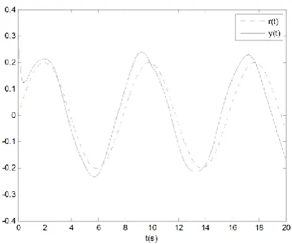
Figure 2.𝑟(𝑡) and 𝑦(𝑡) without actuator failures

𝐵 = [

0.0001 0.018

0 −0.3178

0 −0.0237

0 0

],

𝐷 = [ 0.001 0.001 0.001

0

], 𝐶 = [ 0 0 0 1

] ,

where 𝑥(𝑡) = [𝑢 𝑤 𝑞 𝜃] is the state vector which is composed of linear velocities 𝑢 and 𝑤 (along 𝑋 and 𝑍 body axes, respectively), angular velocities 𝑞 (around 𝑌 body axes) and pitch angle 𝜃; 𝑢(𝑡) = [𝑛 𝛿 ] is the control input which is composed of engine speed n and elevator angle 𝛿 ; 𝑦(𝑡) = 𝜃 is the output; 𝑤(𝑡) ∈ 𝐿 [0, ∞) is the exogenous disturbance. 𝜆 and 𝜆 are system parameter uncertainties satisfying |𝜆 | ≤ 𝜆̅ = 0.012 and |𝜆 | ≤ 𝜆̅ = 0.01 . Then, the system (25) can be represented by a four-vertex polytopic system.

For simulation, we assume 𝑆 = 1, ℎ = 10𝑚𝑠, 𝑤(𝑡) = 0.0 sin 3𝑡 and 𝑟(𝑡) = 0.2 sin 0.8𝑡 . In addition, the initial state of the longitudinal airship system is assumed to be [0.1 0 0 0.3] .

Case 1. Without considering the actuator failures, that is 𝜃 = 𝜃 = 1 . By solving the convex optimization problem formulated in Remark 5, the

obtained minimum guaranteed 𝐻 tracking

performance is min 𝛾 = 2. 204 and the admissible controller gain matrices are as follows:

𝐾 = [ 0.0101 −3.4 1 18.7102 −2. 0 1 −0.0347 −2.8 3 30.481 −0.0387], 𝐾 = [1. 1 0

2. 7 8].

The output 𝑦(𝑡) and the reference output signal 𝑟(𝑡) are shown in Fig. 2, from which we can see that 𝑦(𝑡) tracks 𝑟(𝑡) well with parameter uncertainties.

Figure 3.𝑟(𝑡) and 𝑦(𝑡) with probabilistic actuator failures

Case 2. Considering the probabilistic actuator failures, setting 𝜃 ∈ {0.4, 1, 1.3} and 𝜃 ∈ {0. , 1, 1. } with probabilities given by

𝑃𝑟𝑜𝑏{𝜃 = 0.4} = 𝑃𝑟𝑜𝑏{𝜃 = 0. } = 0.1, 𝑃𝑟𝑜𝑏{𝜃 = 1} = 𝑃𝑟𝑜𝑏{𝜃 = 1} = 0.8, (26) 𝑃𝑟𝑜𝑏{𝜃 = 1.3} = 𝑃𝑟𝑜𝑏{𝜃 = 1. } = 0.1. By solving the corresponding optimization problem, the obtained minimum guaranteed 𝐻 tracking performance is 𝛾 = 2. 731 and the admissible controller gain matrices are given by

𝐾 = [0.041 −8.4 1_{0.001 −4.82 13.74 3 −4.84 1}7. 827 − . 247],

𝐾 = [0.4 37_{1.28 4}].

The output 𝑦(𝑡) and the reference output signal 𝑟(𝑡) are shown in Fig. 3. From Fig. 3, it can be seen that 𝑦(𝑡) tracks 𝑟(𝑡) well with both probabilistic actuator failures and parameter uncertainties.

6. Conclusions

(8)

Funding

This work was supported by the National Natural Science Foundation of China (Grant Number 11272205).

References

[1] D. M. Dawson, Z. Qu, J. J. Carroll. Tracking control of rigid-link electrically-driven robot manipulators. International Journal of Control, 1992, Vol. 56, No. 5, 991-1006.

[2] D. Ye, G. H. Yang. Adaptive fault-tolerant tracking control against actuator faults with application to flight Control. IEEE Transactions on Control Systems Technology, 2006, Vol. 14, No. 6, 1088-1096. [3] Y. Xia, Z. Zhu, M. Fu, S. Wang. Attitude tracking of

rigid spacecraft with bounded disturbances. IEEE Transactions on Industrial Electronics, Vol. 58, No. 2, 647-659, 2011.

[4] F. Liao, J. L. Wang, G. H. Yang. Reliable robust flight tracking control: an LMI approach. IEEE Transactions on Control Systems Technology, 2002, Vol. 10, No. 1, 76-89.

[5] J. Hu, D. M. Dawson, Y. Qian. Position tracking control of an induction motor via partial state feedback. Automatica, 1995, Vol. 31, No. 7, 989-1000. [6] N. C. Shieh, P. C. Tung, C. L. Lin. Robust output tracking control of a linear brushless DC motor with time varying disturbances. In: IEE Proceedings-Electric Power Applications, 2002, Vol. 149, No. 1, pp. 39-45.

[7] H. Gao, T. Chen. Network-based H1 output tracking control. IEEE Transactions on Automatic Control, 2008, Vol. 53, No. 3, 655-667.

[8] C. Lin, Q. G. Wang, T. H. Lee. H1 output tracking control for nonlinear systems via T-S fuzzy model approach. IEEE Transactions on Systems, Man, and Cybernetics-Part B: Cybernetics, 2006, Vol. 36, No. 2, 450-457.

[9] M. Deng, N. Bu, A. Inoue. Output tracking of nonlinear feedback systems with perturbation based on robust right coprime factorization. International Journal of Innovative Computing, Information and Control, 2009, Vol. 5, No. 10, 3359-3366.

[10] E. Fridman, A. Seuret, J. P. Richard. Robust sampled-data stabilization of linear systems: An input delay approach. Automatica, 2004, Vol. 40, No. 8, 1441-1446.

[11] E. Fridman. A refined input delay approach to sampled-data control. Automatica, 2010, Vol. 46, No. 2, 421-427.

[12] H. Gao, J. Wu, P. Shi. Robust sampled-data 𝐻 control with stochastic sampling. Automatica, 2009, Vol. 45, No. 7, 1729-1736.

[13] M. Liu, J. You, X. Ma.𝐻 filtering for sampled-data stochastic systems with limited capacity channel. Signal Processing, 2011, Vol. 91, No. 8, 1826-1837. [14] P. Shi. Filtering on sampled-data systems with

para-metre uncertainty. IEEE Transactions on Automatic Control, 1998, Vol. 43, No. 7, 1022-1027.

[15] Z. Wang, B. Huang, P. Huo. Sampled-data filtering with error covariance assignment. IEEE Transactions on Signal Processing, 2001, Vol. 49, No. 3, 666-670. [16] G. Yang, D. Ye. Reliable 𝐻 control of linear systems

with adaptive mechanism. IEEE Transactions on Automatic Control, 2010, Vol. 55, No. 1, 242-247. [17] Z. Zuo, D. W. C. Ho, Y. Wang. Fault tolerant control

for singular systems with actuator saturation and non-linear perturbation. Automatica, Vol. 46, No. 3, 569-576.

[18] Z. Xiang, R. Wang, Q. Chen. Robust 𝐻 reliable control for a class of switched nonlinear systems with time delay. International Journal of Innovative Computing, Information and Control, 2010, Vol. 6, No. 8, 3329-3338.

[19] E. Tian, D. Yue, C. Peng. Reliable control for networked control systems with probabilistic sensors and actuators faults. IET Control Theory and Application, 2010, Vol. 4, No. 8, 1478-1488.

[20] Z. Gu, J. Liu, C. Peng, E. Tian. Fault-distribution dependent reliable control for T-S fuzzy time delayed systems. Journal of Dynamics Systems, Measurement, and Control, 2011, Vol. 133, No. 6, doi:10.1115/1.4004066.

[21] Z. Gu, D. Wang, D. Yue. New method of fault-distribution-dependent memory-reliable controller design for discrete-time systems with stochastic input delays. IET Control Theory and Applications, 2011, Vol. 5, No. 1, 38-46.