R E S E A R C H A R T I C L E
Open Access
A numerical shallow-water model for
gravity currents for a wide range of density
differences
Hiroyuki A. Shimizu
*, Takehiro Koyaguchi and Yujiro J. Suzuki
Abstract
Gravity currents with various contrasting densities play a role in mass transport in a number of geophysical situations. The ratio of the density of the current,ρc, to the density of the ambient fluid,ρa, can vary between 100and 103. In this paper, we present a numerical method of simulating gravity currents for a wide range ofρc/ρausing a shallow-water model. In the model, the effects of varyingρc/ρaare taken into account via the front condition (i.e., factors describing the balance between the driving pressure and the ambient resistance pressure at the flow front). Previously, two types of numerical models have been proposed to solve the front condition. These are referred to here as the Boundary Condition (BC) model and the Artificial Bed (AB) model. The front condition is calculated as a boundary condition at each time step in the BC model, whereas it is calculated by setting a thin artificial bed ahead of the front in the AB model. We assessed the BC and AB models by comparing their numerical results with the analytical results for a simple case of homogeneous currents. The results from the BC model agree well with the analytical results whenρc/ρa102, but the model tends to overestimate the speed of the front position whenρc/ρa102. In contrast, the AB model generates good approximations of the analytical results forρc/ρa 102, given a sufficiently small artificial bed thickness, but fails to reproduce the analytical results whenρc/ρa102. Therefore, we propose a numerical method in which the BC model is used for currents withρc/ρa102and the AB model is used for currents withρc/ρa102.
Keywords: Gravity currents, Numerical model, Shallow-water model, Front condition
Introduction
Gravity currents are flows driven by density differences between the current and the ambient fluid. In geophysical settings, there are many types of high-Reynolds-number (typically 103) gravity currents that show a wide range
of density ratios (ρc/ρa, whereρc and ρa are the
densi-ties of the current and ambient fluid, respectively), such as debris flows (ρc/ρa∼103; e.g., Iverson 1997), turbidity
currents (ρc/ρa ∼ 100; e.g., Meiburg and Kneller 2010),
and pyroclastic density currents (ρc/ρa =100–101in the
overlying parts andρc/ρa = 102–103 in the underlying
parts; e.g., Branney and Kokelaar 2002; Breard et al. 2016; Nield and Woods 2004). For the two extreme cases of ρc/ρa ∼ 100 and 103, the fluid dynamical features of
gravity currents (e.g., the shape of the interface and the propagation of the flow front) have been studied in detail
*Correspondence: [email protected]
Earthquake Research Institute, The University of Tokyo, 1-1-1 Yayoi, 113-0032 Bunkyo-ku, Tokyo, Japan
using experimental investigations (e.g., Marino et al. 2005; Martin and Moyce 1952; Dressler 1954; Rottman and Simpson 1983), numerical investigations (e.g., Cantero et al. 2007; Ooi et al. 2009), and theoretical modeling (e.g., Benjamin 1968; Hogg and Pritchard 2004; Huppert and Simpson 1980; Stoker 1992; Ungarish and Zemach 2005). For intermediate density ratios (100< ρ
c/ρa<103), there
have been some previous studies (e.g., Birman et al. 2005; Bonometti et al. 2011; Gröbelbauer et al. 1993; Hallworth and Huppert 1998; Härtel et al. 2000; Ungarish 2007), but the dynamics of gravity currents within this density range is less well understood than that of the extreme cases.
The purpose of this study is to develop a numer-ical model of gravity currents for a wide range of ρc/ρa based on a water model. The
shallow-water model is an efficient mathematical model that captures the essential features of the vertically aver-aged motion of gravity currents with free surfaces (see
Ungarish 2009 for an extensive review). For simple ini-tial and boundary conditions, analytical solutions of the shallow-water model for propagating gravity currents are available for a wide range of ρc/ρa (Ungarish 2007),
and these analytical solutions have been verified by experimental measurements and direct numerical simu-lations using the Navier–Stokes equation (Bonometti and Balachandar 2010; Ungarish 2007). However, geophysical conditions of interest generally have rather complex initial and boundary conditions, so such analytical solutions are not always available. A numerical model that is applica-ble for complex initial and boundary conditions is highly desirable for simulations of gravity currents for a wide range ofρc/ρa.
This study is particularly concerned with a numerical treatment of the flow front of gravity currents. In the fol-lowing sections, we formulate the mathematical problem and show that the numerical treatment at the flow front is key to correctly solving the dynamics of gravity cur-rents for a wide range ofρc/ρa within the framework of
the shallow-water model. We also assess previous numer-ical methods that have been used to calculate the behavior of the flow front by comparing numerical and analytical results, and we propose a numerical method to simulate the dynamics of gravity currents for a wide range ofρc/ρa
under various geophysical conditions. Finally, as a geo-physical application of our results, we develop a numerical model of a pyroclastic density current with strong density stratification.
Methods
Formulation
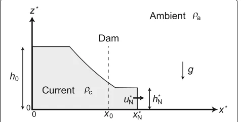
We consider a planar, inviscid, incompressible, immisci-ble gravity current of densityρc in a deep ambient fluid
of densityρa, as shown in Fig. 1. The current propagates
along a smooth horizontal bottom in the positivex∗ direc-tion in timet∗, and gravitational accelerationgacts in the negativez∗direction, where asterisks denote dimensional variables. The propagating current is initially stationary in a reservoir of lengthx0and heighth0, and propagation
Fig. 1Schematic of the gravity current released from a dam in a deep ambient fluid
occurs after a dam atx∗=x0is rapidly removed att∗=0.
The boundary atx∗ = 0 is a rigid wall. The flow front at x∗ = x∗N(t∗)is affected by the resistance of the ambient fluid, where N denotes the front. This problem is referred to as the “dam-break problem” (e.g., Ungarish 2009), and is a simple geophysical scenario.
We assume that the current is shallow, withh0/x01,
and is in hydrostatic equilibrium in the vertical direction (i.e., the water approximation). In the shallow-water approximation, we can obtain the vertically aver-aged conservation equations of mass and momentum for the flow interiorx∗<x∗N(e.g., Ungarish 2007) as follows:
∂h∗ ∂t∗ +
∂ ∂x∗(u
∗h∗)=0, (1)
∂
∂t∗(u∗h∗)+ ∂x∂∗
u∗2h∗+1 2
ρc−ρa
ρc
gh∗2
=0, (2)
where h(x,t) is the local height and u(x,t) is the local horizontal velocity.
At the flow frontx∗ = x∗N(t∗), the kinematic condition (dx∗N/dt∗ = u∗N) and the mass and momentum equations should be taken into account. In addition, to describe realistic gravity current dynamics, we must consider a quasi-steady balance between the buoyancy pressure driv-ing the current front (∼ (ρc−ρa)gh∗N) and the resistance
pressure caused by the acceleration of the ambient fluid around the front (∼ ρau∗N2). This condition is known as
the front condition, and can be written as follows (e.g., Ungarish 2007):
u∗N=Fr
ρc−ρa
ρa
gh∗N at x∗=x∗N(t∗), (3)
where Fr, which is an imposed frontal Froude num-ber, is assumed to be a constant of order 100 (e.g.,√2; Benjamin 1968).
Here, usingx0as the length scale andh0as the height
scale, we rewrite all dimensional variables to dimension-less variables as follows:
x=x∗/x0, h=h∗/h0, u=u∗/U, t=t∗/T, (4)
with
U=
ρc−ρa
ρc
gh0, T =x0/U. (5)
Applying this scaling to Eqs. (1)–(3), we obtain ∂
∂tq+ ∂
∂xf =0 (6)
uN=Fr
ρc/ρa
hN at x=xN(t) (7)
with q= h uh ; f =
uh u2h+ 12h2
. (8)
Note that the density ratioρc/ρa is included only in the
it is important to calculate the front condition correctly (Ungarish 2007).
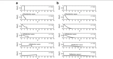
The behavior of the analytical solutions for the above equations depends onρc/ρa(Fig. 2; Ungarish 2007). The
analytical solutions of the dam-break problem consist of an initial “slumping” stage and a subsequent “self-similar” stage (Fig. 2a; e.g., Hogg 2006). During the slumping stage, the front moves with a constant speed and height. Dur-ing this stage, an initial backward-propagatDur-ing rarefaction wave arises from the rapidly removed dam, and then a wave arises from the reflection of this rarefaction wave at the back wallx = 0 att = 1. The slumping stage con-tinues until the front is caught by this reflection wave. After the slumping stage, the solution is asymptotic to a similar solution as time tends to infinity (i.e., the self-similar stage). During this stage, the velocity and height of the front decrease with time. The dependence of the solu-tion onρc/ρa is clearly observed in the behavior of the
flow front. Whenρc/ρa ∼ 100, the front heighthNis on
the order of 10−1 during the slumping stage and in the early self-similar stage (Fig. 2a). On the other hand, when ρc/ρa ∼ 103, hNis much smaller than 10−1, even from
the beginning, the front velocityuNis substantially greater
thanuNforρc/ρa ∼ 100(Fig. 2b). These differences can
be interpreted as follows: the momentum lost due to the
resistance of the ambient fluid at the front becomes less significant with respect to the momentum of the current asρc/ρaincreases. We aim to numerically reproduce these
features of the analytical solution below.
Numerical methods
In this study, we developed a numerical method for modeling gravity currents for a wide range of ρc/ρa by
discretizing the dimensionless mass and momentum con-servation equations (Eqs. (6) and (8)). As these equations are nonlinear and hyperbolic, shocks may develop in the currents. Consequently, we used a finite volume method with shock-capturing capability (e.g., LeVeque 2002; Toro 2001). The finite volume method updates a piecewise constant functionQni that approximates the average value of the solutionqin each grid celliat time stepn, using the expression
Qni+1=Qni − t
x(Fi+1/2−Fi−1/2), (9) wherexis the constant cell length andtis the time interval.Fi+1/2, which is the intercell flux between cellsi
andi+1, is obtained by using an exact Riemann solver or an approximate Riemann solver, such as the Roe scheme (e.g., LeVeque 2002; Toro 2001). The time intervaltis
limited by the Courant–Friedrichs–Lewy condition (e.g., LeVeque 2002; Toro 2001).
As mentioned above, if we are to capture the effects of ρc/ρa, it is important to calculate the front condition (7)
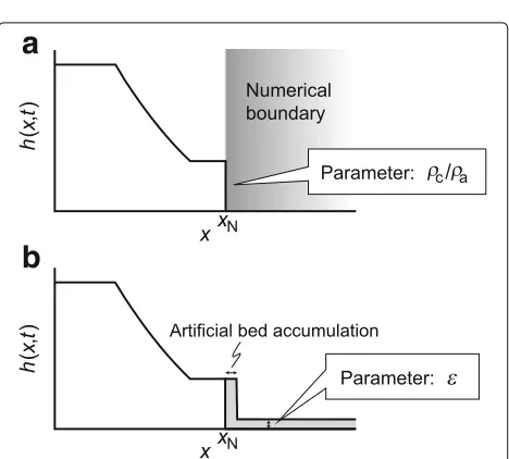
correctly. Previously, two types of numerical models have been proposed to calculate the front condition. In one, the front condition is calculated as a boundary condition at each time step (e.g., Ungarish 2009). We refer to this model as the Boundary Condition (BC) model (Fig. 3a). In the other, the front condition is calculated by setting a thin artificial bed ahead of the front (e.g., Toro 2001). We refer to this as the Artificial Bed (AB) model (Fig. 3b). In the AB model, the resistance of the ambient fluid at the flow front is modeled by the reaction of the force pushing the artificial bed at the flow front. These models will be described below.
Boundary Condition (BC) model
In the BC model, three quantities at the flow front (xN,
hN, anduN) are calculated as boundary conditions of the
current from the three equations (mass and momentum conservation equations and front condition) at each time step. In the present numerical method, because we apply a fixed spatial coordinate with constant x, the front positionx = xN(t) generally does not coincide with the
margins of the grid cells. We therefore define the cell that includes the front as the front cell (i=FC(t), whereFC(t) is an integer), and the width of the region that the current occupies in the front cell asxFC(t)(0≤xFC(t) < x; see Fig. 4). Using FC(t) and xFC(t), we can write the front position as
xN(t)=(FC(t)−1)x+xFC(t). (10)
Fig. 3Schematics of the numerical models used to calculate the front condition.aBoundary Condition (BC) model.bArtificial Bed (AB) model
The values ofhNanduNare approximated by the values
ofhanduat the front cell (i.e.,hFCanduFC).
When the kinematic condition (dxN/dt = uN) is taken
into account, the discretized equations for mass and momentum conservation at the flow front are given by
xnFC+1hnFC+1=xnFChnFC+tf1 (11)
and
xn+1
FC (uh)nFC+1=xnFC(uh)nFC+t
f2−
1 2
hnFC+1
2
,
(12)
respectively, where (f1,f2)T represents the intercell flux FFC−1/2. From the front condition (i.e., Eq. (7)), we obtain
(uh)nFC+1 hnFC+1 =Fr
ρc/ρa
hnFC+1. (13)
Solving these three equations analytically (e.g., using Fer-rari’s method for the solution of the quartic equation) or numerically (e.g., using the Newton–Raphson iteration method), we obtain hnFC+1, uFCn+1, andxnFC+1, and hence, hN,uN, andxNat each time step.
Artificial Bed (AB) model
In the AB model, the conservation equations (Eqs. (6) and (8)) are numerically solved using a shock-capturing method for not only the interior, but also the outside of the current by a priori setting a thin artificial bed ahead of the front. Through this numerical procedure, the flow front is generated as the flow following a shock formed ahead of the front without any additional calculation (see Fig. 3b). In this model, the thickness of the artificial bed (εin Fig. 3b) is the parameter that controls the front con-dition (i.e., the values ofhNanduNfor different values of
ρc/ρa; see section 10.8 in Toro 2001).
Here, we analytically determined the relationship betweenεandρc/ρa, as well as that betweenuNandε, on
the basis of the analytical solution for the slumping stage of the dam-break problem (e.g., LeVeque 2002; Toro 2001; Ungarish 2009). The initial conditions areh=1 andu=0 in the domain 0 ≤ x ≤ 1, andh = εandu = 0 in the domainx > 1, att = 0. Let us consider the time evolu-tion of the current before the rarefacevolu-tion wave reaches the back wallx=0 (i.e., 0<t≤1).
For hyperbolic equations such as those used in the present system (i.e., Eqs. (6) and (8)), the relationships between the variables (i.e.,handu) on the characteristics c±=u±√hare represented as follows:
±=u±2√h=const on dx
con-Fig. 4Schematic of the computational domain of the BC model
dition (h = 1,u = 0) enter the front domain (h = hN,
u=uN), we can obtain
uN=2
1−hN
(15)
from Eq. (14). The equation provides the relationship betweenh=hNandu=uNinside the current.
On the other hand, when an artificial bed withh=εand u = 0 is set, a shock wave traveling with speedSoccurs ahead of the front. Across this shock wave, the Rankine– Hugoniot condition,
f(qR)−f(qL)=S(qR−qL) (16)
should hold. Here, the subscript R denotes the state on the right side of the shock and L denotes the state on the left side. From Eq. (16), we obtain the state of the front domain behind the shock (i.e., the relationship betweenh = hN
andu=uN) as
uN=(hN−ε)
1 2
hN+ε
hNε
, (17)
and the shock speed as
S=
1 2
(hN+ε)hN
ε . (18)
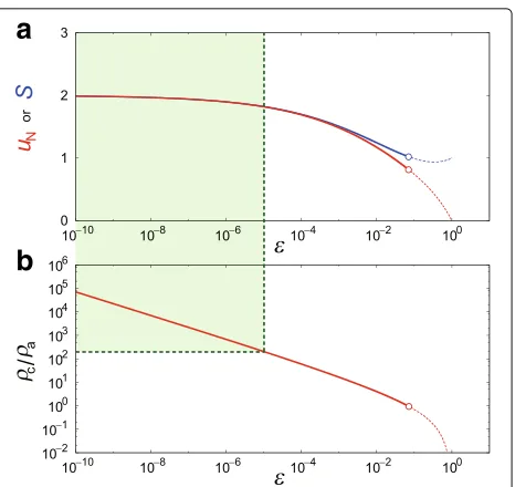
EliminatinghNfrom Eqs. (15), (17), and (18), we obtain
uNandSas a function ofε(Fig. 5a). Using the front
con-dition (7) as well as these equations, we also obtain the relationship between the artificial bed thicknessεand the density ratioρc/ρa(Fig. 5b) as
1− 2
Fr√ρc/ρa+2
4√2ε
Fr√ρc/ρa+2
=
2
Fr√ρc/ρa+2 2
−ε
2
Fr√ρc/ρa+2 2
+ε.
(19)
Note that because we use Eq. (15) here, these relationships (Fig. 5) are in the slumping stage.
In Fig. 5a,Sis larger than the front velocity,uN, because
of the accumulation of the artificial bed at the flow front (see Fig. 3b). This deviation ofSfromuNis substantial for
ε10−3. This implies that the position of the shock does not always approximate the flow front. If we are to extract the correct position of the flow front, we must calculate an advection equation for a passive tracer concentration, φ(φ =1 for 0≤x≤1, andφ=0 forx>1, att=0):
∂φ ∂t +u
∂φ
∂x =0 (20)
after solving the equations of fluid motion (see section 13.12 in LeVeque 2002 for details).
Results and discussion
In this section, we compare the numerical results obtained from the BC and AB models with the analytical results, and assess the applicability of these models. Subsequently, as a geophysical application of our results, we develop a numerical model of pyroclastic density currents.
Fig. 5Analytical solutions for the AB model during the slumping stage.aFront velocityuN(red curve) and shock speedS(blue curve), as functions ofε.bRelationship betweenεandρc/ρa, in which
Comparison of analytical and numerical results
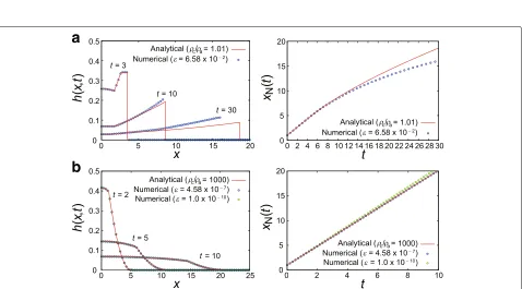
Figure 6 shows the numerical results from the BC model along with the analytical results for the cases ofρc/ρa =
1.01 (a) and 1000 (b). The numerical results forρc/ρa =
1.01 agree well with the analytical results from the early slumping stage to the late self-similar stage. The numer-ical results forρc/ρa = 1000 also appear to agree with
the analytical results, but the speed of the front position, ˙
xN, shows a numerical oscillation that is not observed in
the analytical result (Fig. 7a). In particular, in the initial stage (t 0.0002 in Fig. 7a), x˙N tends to be
overesti-mated. These oscillation and overestimation are caused by the assumption that the values of hFC and uFC are uniform across the width of the front cell xFC in the present numerical method at first-order accuracy. For a large ρc/ρa, because hN has a small value, the value of
xFC tends to be overestimated when a constant hFC is assumed (Fig. 7b). We suggest, therefore, that the BC model is favorable for simulating gravity currents with relatively lowρc/ρa.
Figure 8 shows the numerical results from the AB model along with the analytical results. In these calculations, the values ofεfor given values ofρc/ρaare set based on the
relationship of Eq. (19) (see Fig. 5b). In Fig. 8b, the numer-ical results for ρc/ρa = 1000 (ε = 4.58×10⁻⁷) agree
well with the analytical results. The numerical oscilla-tions observed in the BC model do not occur with the AB model (Fig. 7a). In Fig. 8a, on the other hand, the numer-ical results for ρc/ρa = 1.01 (ε = 6.58× 10⁻²) agree
well with the analytical results only during the slumping
stage (t 4.5), but deviate from the analytical results during the self-similar stage (t 4.5). This agreement during the slumping stage and deviation during the self-similar stage occurs becauseεis set using the analytical relationship (Eq. (19)) for the slumping stage of the dam-break problem. During the slumping stage,hNanduNare
constant so thatεbased on Eq. (19) provides the correct front condition. During the self-similar stage, on the other hand, the driving pressure, and hencehNanduN, decrease
with time; therefore, the assumed value ofεis no longer consistent with the front condition Eq. (7).
The good agreement in the results of the AB model for ρc/ρa = 1000 reflects the fact that the dynamics of the
gravity current becomes insensitive to the front condition for large values of ρc/ρa. In Fig. 5b, ε approaches 0 as
ρc/ρaincreases. In the limit asρc/ρa → ∞andε → 0,
uNasymptotically approaches its maximum value, 2, and
hNasymptotically approaches 0. For sufficiently small ε,
the solution converges to that in the limit as uN → 2
andhN → 0, and it becomes insensitive to the value of
ε(see Fig. 5a). Indeed, as shown in Fig. 8b, we can con-firm that the result of the AB model with a very small ε (ε = 1.0× 10⁻¹⁰) is indistinguishable from that for ρc/ρa = 1000 (ε = 4.58× 10⁻⁷). According to Fig. 5,
the results of the AB model for the dam-break problem are insensitive toε whenε 10−5, which corresponds to ρc/ρa 102(Fig. 5b). Consequently, we suggest that
the AB model is favorable for simulating gravity currents with highρc/ρafor which the dynamics of the current is
insensitive to the assumed value ofε.
Fig. 7Speed of the front position,x˙N, in the early time steps.aComparisons between the analytical result withρc/ρa=1000 (red line) and numerical results of the BC model withρc/ρa=1000 (blue symbols) and of the AB model withε=4.58×10⁻⁷(green symbols). In the numerical calculations,x=1.0×10⁻⁴.bIllustrations of the overestimation ofx˙
Nby the BC model int0.0002 in (a)
Fig. 8Analytical results (red curves) and numerical results of the AB model (symbols) forh(x,t)andxN(t).aρc/ρa=1.01.bρc/ρa=1000. In the numerical results,blue symbolsrepresent the numerical results givenεbased on the analytical solution during the slumping stage (aε=6.58×10⁻²;
Applicability of the BC and AB models
Our results indicate that the BC and AB models each have their own advantages and disadvantages. The results obtained from the BC model agree well with the analyti-cal results whenρc/ρa102(Fig. 6a), whereas they show
a numerical oscillation at the flow front and tend to over-estimate the front speed whenρc/ρa 102(Fig. 7). No
such numerical oscillation nor overestimation is observed in the results from the AB model. For currents with ρc/ρa 102, the AB model provides good
approxima-tions of the analytical results, given a sufficiently smallε (Figs. 5 and 8b). For currents withρc/ρa 102, however,
the AB model may fail to reproduce the analytical results for currents where the height and speed of the front change with time (Fig. 8a). Accordingly, we propose that the BC model should be used for currents withρc/ρa
102 and the AB model is applicable only to currents withρc/ρa102.
Because of its simple coding and numerical stability, the AB model with an arbitrarily small ε is commonly used for simulations of gravity currents in many geophys-ical situations (e.g., Denlinger and Iverson 2004; Doyle et al. 2007, 2008, 2011; Larrieu et al. 2006). This model would be applicable in simulating gravity currents with high values ofρc/ρa, such as debris flows (e.g., Denlinger
and Iverson 2004). However, our results suggest that it may provide inaccurate results for gravity currents with ρc/ρa 102, such as turbidity currents and dilute
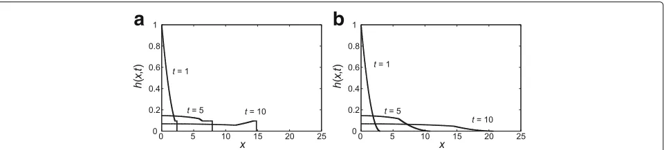
pyro-clastic density currents. Numerical results forρc/ρa =10
show that the problem arises mainly from the behavior of the flow front (Fig. 9). Generally, a gravity current with a relatively low value ofρc/ρa is characterized by the
for-mation of a large front height, which is caused by the resistance of the ambient fluid. This large front height is successfully reproduced by the BC model (Fig. 9a), while the AB model fails to capture it. The results from the AB model with ε = 10−10 (Fig. 9b) show that the resistance at the front is too small to develop a large front height; consequently, the flow speed is substantially overestimated.
Geophysical application to pyroclastic density currents Pyroclastic density currents (PDCs) are characterized by strong density stratification due to particle settling (e.g., Branney and Kokelaar 2002), whereby a dilute gravity cur-rent (particle suspension flow) with ρc/ρa = 100–101
overrides the dense basal gravity current (fluidized gran-ular flow) withρc/ρa =102–103. The dynamics of PDCs
is complex because the dilute and dense currents are influenced by a number of physical processes such as par-ticle settling (e.g., Bonnecaze et al. 1993), entrainment of ambient air (e.g., Johnson and Hogg 2013; Sher and Woods 2015), and basal resistance (e.g., Roche et al. 2008). In addition to the effects of these processes, our results suggest that the application of the correct numerical model to the flow front is important if we are to under-stand the dynamics and sedimentation of PDCs. The BC model should be applied to the overlying dilute current, while the AB model is applicable to the underlying dense current. Here, we discuss how the resistance at the flow front of the dilute part influences the dynamics of PDCs as a whole.
Before discussing the complex dynamics of PDCs with strong density stratification, we briefly assess the effects of some important physical processes on the dilute and dense currents. Figure 10 shows the results of simula-tions using the BC model for a dilute gravity current generated by an instantaneous release (i.e., the dam-break problem) of an initially homogeneous particle suspen-sion with ρc/ρa = 8.495. This model accounts for the
effects of particle settling and entrainment of the ambi-ent fluid following Bonnecaze et al. (1993) and Johnson and Hogg (2013), respectively. As with a homogeneous gravity current with a low density ratio (Fig. 6a), a thick front develops in the dilute gravity current of the particle suspension, suggesting that the resistance of the ambient fluid at the front plays a significant role in the dynamics of the dilute part of PDCs regardless of the presence or absence of the effects of particle settling or entrainment.
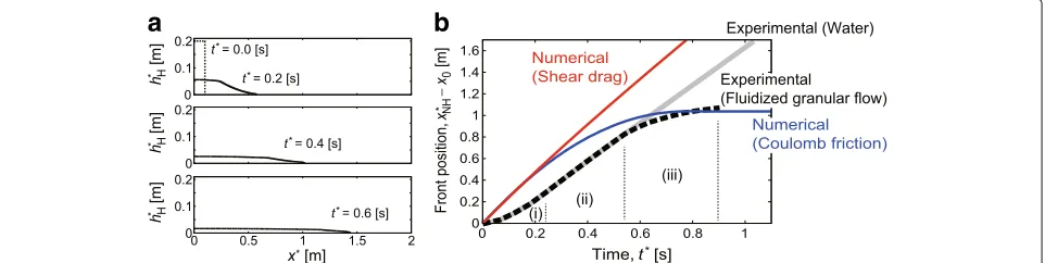
Figure 11 compares our numerical results obtained using the AB model with experimental results for a
Fig. 10Numerical results of a one-layer dilute PDC model for the dam-break problem. HeightshLatat=1 andbt=10 are shown for cases of entraining (solid curves) and non-entraining (dotted curves) currents. The initial density ratio (ρL∗/ρa) is set to 8.495, and the BC model is applied. The variables are non-dimensionalized using the initial values (e.g., Eqs. (4) and (5)). Given parameters: aspect ratio (initial height/initial length)=1; initial particle concentration=0.005; density ratio (particles/air)=1500; density ratio (volcanic gas/air)=1; and non-dimensional particle settling speed
=0.05
granular flow with ρc/ρa = 102–103 generated by an
instantaneous release of an initially fluidized bed (Roche et al. 2008). Because the initial acceleration regime of the experimental setup (i.e., just after the release; (i) in Fig. 11b) is beyond the applicable range of the shallow-water model, we focus on the subsequent regimes here. The numerical results obtained using the AB model show the formation of a wedge-shaped flow front (Fig. 11a), which is in agreement with the experimental results of Roche et al. (2008). The results also indicate that the dynamics of the dense fluidized granular flow can be quantitatively simulated by the AB model when a suit-able rheological model is applied for the basal resistance (Fig. 11b). The shear drag model explains the behavior during the constant velocity regime ((ii) in Fig. 11b; see Roche et al. 2008), whereas the Coulomb friction model better reproduces the features of the stopping regime ((iii) in Fig. 11b; see Roche et al. 2008).
The interplay between the dilute and dense parts may be crudely simulated by a two-layer model comprising a dilute layer and a dense layer (Doyle et al. 2008, 2011).
The previous two-layer models for PDCs apply the AB model with a smallεto both layers. Here, we follow Doyle et al. (2011) for the basic formulation of the two-layer sys-tem, but apply the BC model to the dilute layer and the AB model to the dense layer. We also consider the effects of basal shear drag in the dense layer and entrainment of ambient air into the dilute layer (see Appendix for details). Figure 12 shows a representative result of our two-layer model for a PDC generated by the instantaneous release of an initially homogeneous dilute particle suspension with ρc/ρa = 8.495. When the BC model is applied, a thick
front head develops in the dilute gravity current because of the resistance of the ambient fluid at the front (see Fig. 10). On the other hand, a dense gravity current with ρc/ρa = 600.6 is generated by particle settling from the
overlying dilute gravity current. Because the rate at which particles are supplied to the dense layer is controlled by the conditions of the overlying dilute layer (e.g., thickness and particle concentration), the evolution and dynamics of the dense layer are critically dependent on those of the dilute layer. This suggests that the behavior of the flow
Fig. 12Numerical results of a two-layer PDC model for the dam-break problem. The dense current height (hH) and dilute current height (hL+hH) at
at=1 andbt=10 are shown. A PDC is generated by the instantaneous release of an initially homogeneous dilute layer. The overlying dilute layer (initiallyρL∗/ρa=8.495) is calculated using the BC model, and the underlying dense layer (ρH/ρa=600.6) is calculated using the AB model with
ε=10−10. Shear drag is applied for the basal resistance of the dense layer. The variables are non-dimensionalized using the initial values of the dilute layer (e.g., Eqs. (4) and (5)). Given parameters: aspect ratio (initial height/initial length) = 1; initial particle concentration of the dilute layer
=0.005; density ratio (particles/air)=1500; density ratio (volcanic gas/air)=1; and the non-dimensional particle settling speed=0.05
front of the dilute layer controls not only the dynamics of the dilute layer but also the dynamics of the stratified PDC as a whole.
The results in Fig. 12 are preliminary, and a compre-hensive understanding of the dynamics of PDCs should consider many other effects, such as the expansion of entrained air due to heating by pyroclasts, density strat-ification inside the overlying dilute layer, diffusion of the pore pressure and entrainment of air in the under-lying dense layer, and the transport of particles from the underlying dense layer to the overlying dilute layer (e.g., Andrews 2014; Breard and Lube 2017; Bursik and Woods 1996; Dufek and Bergantz 2007; Esposti Ongaro et al. 2016; Ishimine 2005; Roche et al. 2008; Wilson and Walker 1982). Nevertheless, preliminary results (not shown here) have already indicated the diversity of the interplay between the dilute and dense layers, which depends on the initial particle concentration and grain size. The interaction also influences the sedimentation process from the PDCs (Fujii and Nakada 1999). A system-atic parametric study of the two-layer PDC model using the BC model is in progress, with the aim of accounting for the diversity of PDC deposits.
Conclusion
A numerical shallow-water model of simulating gravity currents for a wide range of ρc/ρa has been proposed.
In the model, the effects of varyingρc/ρaare taken into
account via the front condition. We have assessed two types of numerical models for the front condition (the Boundary Condition (BC) model and the Artificial Bed (AB) model) by comparing their numerical results with the analytical results. The results from the BC model agree well with the analytical results when ρc/ρa 102. In
contrast, the AB model generates good approximations of the analytical results for ρc/ρa 102. On the basis
of these results, we have developed a two-layer model
of pyroclastic density currents (PDCs), in which the BC model is used for the overlying dilute part (ρc/ρa =
100–101) and the AB model is used for the underlying
dense part (ρc/ρa=102–103). This two-layer model
suc-cessfully simulates some essential features of PDCs with strong density stratification.
Appendix: two-layer model of pyroclastic density currents
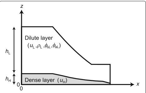
The dynamics of PDCs in which a strong density stratifi-cation develops is described here by a two-layer shallow-water model with overlying dilute and underlying dense layers (Fig. 13). The dilute layer is modeled as a dilute particle suspension, which is a continuum where mono-disperse solid particles are suspended in an incom-pressible gas phase (volcanic gas and entrained air). Its vertically averaged mass and momentum conservation equations are respectively
Fig. 13Two-layer PDC model schematic. In the overlying dilute layer, the thicknesshL, velocityuL, bulk densityρL, particle volume concentrationφsL, and air volume concentrationφaLevolve both temporally and spatially. In the underlying dense layer, the thickness
∂ ∂t∗
ρL∗h∗L
+ ∂
∂x∗
ρL∗u∗Lh∗L
=ρaE|u∗L| −ρHφsL
φsH
Ws, (21)
∂ ∂t∗
ρL∗u∗Lh∗L
+∂∂
x∗
ρL∗u∗L2h∗L+
ρ∗
L−ρa
2 gh ∗2 L
= −ρL∗−ρa
gh∗L∂h
∗
H
∂x∗ −ρH φsL
φsH
u∗LWs−τm∗. (22)
The dense layer, modeled as a fluidized granular flow con-sisting of solid particles and volcanic gas, has the following vertically averaged mass and momentum conservation equations:
∂h∗H ∂t∗ +
∂ ∂x∗
u∗Hh∗H= φsL φsH
Ws,
∂ ∂t∗
u∗Hh∗H+ ∂ ∂x∗
u∗H2hH+
1 2
ρH−ρa
ρH
gh∗H2
(23)
= −τb∗
ρH+
τ∗
m
ρH+
φsL
φsH
u∗LWs−
h∗H ρH
∂ ∂x∗
ρ∗
L−ρa
gh∗L.
(24)
Here,φ(x∗,t∗)is volumetric concentration, and the sub-scripts L, H, s, g, and a denote the dilute (i.e., low-particle concentration) and dense (i.e., high-particle concentra-tion) layers, solid particles, volcanic gas, and air, respec-tively.Ws is the settling velocity of the particles from the
base of the dilute layer,Eis the entrainment coefficient, τ∗
m is the interfacial shear drag, andτb∗is basal resistance
of the dense layer.
The bulk density of the dilute layer is denoted byρL∗ = ρsφsL+ρaφaL+ρg(1−φsL−φaL), in which the volume
con-centrations of the solid particles,φsL, and of the entrained
air,φaL, evolve both temporally and spatially on the basis
of their mass conservation equations: ∂
∂t∗
φsLh∗L
+ ∂
∂x∗
φsLu∗Lh∗L
= −φsLWs, (25)
∂ ∂t∗
φaLh∗L
+ ∂
∂x∗
φaLu∗Lh∗L
=E|u∗L|. (26)
In the dilute layer, it is assumed that turbulent mix-ing is sufficiently intense to maintain vertically uniform volumetric concentrations (e.g., Bonnecaze et al. 1993; Bursik and Woods 1996; Johnson and Hogg 2013). The dense layer is assumed to have a constant bulk density ρH=ρsφsH+ρg(1−φsH), where the particle volumetric
concentrationφsHis set to 0.4 (Breard et al. 2016).
Interactions between the two layers are treated in the source terms of Eqs. (21)–(26) (i.e., the right-hand sides of the equations). Particle settling from the dilute layer to the dense layer is taken into account in the second source terms in Eqs. (21) and (22), the source terms in Eqs. (23) and (25), and the third source term in Eq. (24). The accel-eration of the dilute layer over the basal contact is taken into account in the first source term in Eq. (22). The pres-sure gradient on the dense layer exerted by variations in
the height of the dilute layer is taken into account in the fourth source term in Eq. (24).
The entrainment of ambient air into the dilute layer is taken into account in the first source term in Eq. (21) and the source term in Eq. (26). Thermal expansion of the entrained air is neglected here for the sake of ease. Air entrainment is also assumed to occur on the upper surface of the dilute layer (e.g., Bursik and Woods 1996; Johnson and Hogg 2013), although a different process for entrain-ment was recently proposed by Sher and Woods (2015). We adopted the entrainment coefficient proposed by Johnson and Hogg (2013): i.e.,E=0.075/(1+27Ri), where Ri≡ρL∗−ρa
gh∗L/ρL∗u∗L2.
The interfacial dragτm∗ and the basal resistance of the dense layerτb∗are treated in the source terms in Eqs. (22) and (24). The interfacial shear dragτm∗ is given by (Doyle et al. 2008, 2011):
τm∗ =ρL∗Cd
u∗L−u∗H|u∗L−u∗H|, (27)
where the drag coefficientCd is set to 0.001 (Hogg and
Pritchard 2004). The basal resistanceτb∗is modeled such that shear drag is adopted during the constant velocity regime ((ii) of Fig. 11b) and Coulomb friction is adopted during the stopping regime ((iii) of Fig. 11b):
τ∗
b =
ρHCdu∗H|u∗H| (Shear drag),
tanδ (ρH−ρa)gh∗Hu∗H/|u∗H| (Coulomb friction),
(28)
(Figure 11b; see Roche et al. 2008 for details), where the dynamic basal friction angle δ is set to 20◦ (Doyle et al. 2008).
The front condition of the dilute layer is given by (Ungarish 2007):
u∗NL=Fr ρ
∗
NL−ρa
ρa
gh∗NL at x∗=x∗NL, (29)
which is numerically treated by the BC model. The front condition of the dense layer, given by Eq. (3), is numeri-cally treated by the AB model withε=10−10.
In calculating the two-layer PDC model (Fig. 12), the conservation Eqs. (21)–(26) were numerically solved. In calculating the one-layer dilute PDC model (Fig. 10), we solved conservation Eqs. (21), (22), (25), and (26), where h∗H ≈ 0 andu∗H ≈ 0. In calculating the one-layer dense PDC model (Fig. 11), we solved conservation Eqs. (23) and (24). For numerical simulations, we used a fractional-step method to solve the conservation equations with source terms (e.g., LeVeque 2002), and the HLL approximate Rie-mann solver to calculate the intercell flux of the equations (e.g., Toro 2009).
Abbreviations
Acknowledgements
We thank Editor Colin J. N. Wilson, Reviewer Eric C. P. Breard, and an anonymous reviewer for their thoughtful comments.
Funding Not applicable.
Authors’ contributions
HAS carried out this study under the supervision of TK and YJS and prepared the first draft of the manuscript. All authors contributed to writing the manuscript and approved the final version.
Authors’ information
HAS is a Ph.D. candidate supervised by TK and YJS. TK is a Professor at the Earthquake Research Institute, the University of Tokyo. YJS is an Assistant Professor at the Earthquake Research Institute, the University of Tokyo.
Competing interests
The authors declare that they have no competing interests.
Publisher’s Note
Springer Nature remains neutral with regard to jurisdictional claims in published maps and institutional affiliations.
Received: 21 July 2016 Accepted: 3 March 2017
References
Andrews BJ (2014) Dispersal and air entrainment in unconfined dilute pyroclastic density currents. Bull Volcanol 76:1–14.
doi:10.1007/s00445-014-0852-4
Benjamin TB (1968) Gravity currents and related phenomena. J Fluid Mech 31:209–48. doi:10.1017/S0022112068000133
Birman V, Martin J, Meiburg E (2005) The non-boussinesq lock-exchange problem. part 2. High-resolution simulations. J Fluid Mech 537:125–44. doi:10.1017/S0022112005005033
Bonnecaze RT, Huppert HE, Lister JR (1993) Particle-driven gravity currents. J Fluid Mech 250:339–69. doi:10.1017/S002211209300148X Bonometti T, Balachandar S (2010) Slumping of non-boussinesq density
currents of various initial fractional depths: a comparison between direct numerical simulations and a recent shallow-water model. Comput Fluids 39:729–34
Bonometti T, Ungarish M, Balachandar S (2011) A numerical investigation of high-reynolds-number constant-volume non-boussinesq density currents in deep ambient. J Fluid Mech 673:574–602.
doi:10.1017/S0022112010006506
Branney MJ, Kokelaar BP (2002) Pyroclastic density currents and the sedimentation of ignimbrites. Geol Soc, London
Breard ECP, Lube G (2017) Inside pyroclastic density currents—uncovering the enigmatic flow structure and transport behaviour in large-scale
experiments. Earth Planet Sci Lett 458:22–36. doi:10.1016/j.epsl.2016.10.016 Breard ECP, Lube G, Jones JR, Dufek J, Cronin SJ, Valentine GA, Moebis A (2016) Coupling of turbulent and non-turbulent flow regines within pyroclastic density currents. Nat Geosci 9:767–71. doi:10.1038/NGEO2794 Bursik MI, Woods AW (1996) The dynamics and thermodynamics of large ash
flows. Bull Volcanol 58:175–193. doi:10.1007/s004450050134 Cantero MI, Lee J, Balachandar S, Garcia MH (2007) On the front velocity of
gravity currents. J Fluid Mech 586:1–39. doi:10.1017/S0022112007005769 Denlinger RP, Iverson RM (2004) Granular avalanches across irregular
three-dimensional terrain: 1. theory and computation. J Geophys Res 109:F01014. doi:10.1029/2003JF000085
Doyle EE, Hogg AJ, Mader HM, Sparks RSJ (2008) Modeling dense pyroclastic basal flows from collapsing columns. Geophys Res Lett 35:L04305. doi:10.1029/2007GL032585
Doyle EE, Hogg AJ, Mader HM (2011) A two-layer approach to modelling the transformation of dilute pyroclastic currents into dense pyroclastic flows. Proc R Soc A 467:1348–71. doi:10.1098/rspa.2010.0402
Doyle EE, Huppert HE, Lube G, Mader HM, Sparks RSJ (2007) Static and flowing regions in granular collapses down channels: insights from a sedimenting shallow-water model. Phys Fluids 106601:19. doi:10.1063/1.2773738
Dressler RF (1954) Comparison of theories and experiments for the hydraulic dam-break wave. Int Assoc Sci Hydrol 3:319–28
Dufek J, Bergantz G (2007) Suspended load and bed-load transport of particle-laden gravity currents: the role of particle-bed interaction. Theor Comput Fluid Dyn 21:119–45. doi:10.1007/s00162-007-0041-6 Esposti Ongaro T, Orsucci S, Cornolti F (2016) A fast, calibrated model for
pyroclastic density currents kinematics and hazard. J Volcanol Geotherm Res 327:257–72. doi:10.1016/j.jvolgeores.2016.08.002
Fujii T, Nakada S (1999) The 15 September 1991 pyroclastic flows at Unzen Volcano (Japan): a flow model for associated ash-cloud surges. J Volcanol Geotherm Res 89:159–72. doi:10.1016/S0377-0273(98)00130-9
Gröbelbauer H, Fanneløp T, Britter R (1993) The propagation of intrusion fronts of high density ratios. J Fluid Mech 250:669–87. doi:10.1017/
S0022112093001612
Hallworth MA, Huppert HE (1998) Abrupt transitions in high-concentration, particle-driven gravity currents. Phys Fluids 10:1083. doi:10.1063/ 1.869633
Härtel C, Meiburg E, Necker F (2000) Analysis and direct numerical simulation of the flow at a gravity-current head. part 1. flow topology and front speed for slip and no-slip boundaries. J Fluid Mech 418:189–212.
doi:10.1017/S0022112000001221
Hogg AJ (2006) Lock-release gravity currents and dam-break flows. J Fluid Mech 569:61–87. doi:10.1017/S0022112006002588
Hogg AJ, Pritchard D (2004) The effects of hydraulic resistance on dam-break and other shallow inertial flows. J Fluid Mech 501:179–212.
doi:10.1017/S0022112003007468
Huppert HE, Simpson JE (1980) The slumping of gravity currents. J Fluid Mech 99:785–99. doi:10.1017/S0022112080000894
Ishimine Y (2005) Numerical study of pyroclastic surges. J Volcanol Geotherm Res 139:33–57. doi:10.1016/j.jvolgeores.2004.06.017
Iverson RM (1997) The physics of debris flows. Rev Geophys 35:245–96. doi:10.1029/97RG00426
Johnson CG, Hogg AJ (2013) Entraining gravity currents. J Fluid Mech 731:477–508. doi:10.1017/jfm.2013.329
Larrieu E, Staron L, Hinch E (2006) Raining into shallow-water as a description of the collapse of a column of grains. J Fluid Mech 554:259–70. doi:10.1017/S0022112005007974
LeVeque RJ (2002) Finite volume methods for hyperbolic problems. Cambridge University Press, Cambridge
Marino B, Thomas L, Linden P (2005) The front condition for gravity currents. J Fluid Mech 536:49–78. doi:10.1017/S0022112005004933
Martin JC, Moyce WJ (1952) An experimental study of the collapse of liquid columns on a rigid horizontal plane. Phil Trans R Soc Lond A 244:312–24. doi:10.1098/rsta.1952.0006
Meiburg E, Kneller B (2010) Turbidity currents and their deposits. Annu Rev Fluid Mech 42:135–56. doi:10.1146/annurev-fluid-121108-145618 Nield SE, Woods AW (2004) Effects of flow density on the dynamics of dilute
pyroclastic density currents. J Volcanol Geotherm Res 132:269–81. doi:10.1016/S0377-0273(03)00314-7
Ooi SK, Constantinescu G, Weber L (2009) Numerical simulations of lock-exchange compositional gravity current. J Fluid Mech 635:361–88. doi:10.1017/S0022112009007599
Roche O, Montserrat S, Niño Y, Tamburrino A (2008) Experimental observations of water-like behavior of initially fluidized, dam break granular flows and their relevance for the propagation of ash-rich pyroclastic flows. J Geophys Res 113:B12203. doi:10.1029/2008JB005664
Rottman JW, Simpson JE (1983) Gravity currents produced by instantaneous releases of a heavy fluid in a rectangular channel. J Fluid Mech 135:95–110. doi:10.1017/S0022112083002979
Sher D, Woods AW (2015) Gravity currents: Entrainment, stratification and self-similarity. J Fluid Mech 784:130–62. doi:10.1017/jfm.2015.576 Stoker JJ (1992) Water waves: the mathematical theory with applications.
Wiley, New York
Toro EF (2001) Shock-capturing methods for free-surface shallow flows. Wiley, Chichester
Toro, EF (2009) Riemann solvers and numerical methods for fluid dynamics: a practical introduction. Springer, Berlin
Ungarish M (2007) A shallow-water model for high-reynolds-number gravity currents for a wide range of density differences and fractional depths. J Fluid Mech 579:373–82. doi:10.1017/S0022112007005484 Ungarish M (2009) An introduction to gravity currents and intrusions. CRC
Press, Boca Raton
Wilson CJN, Walker GPL (1982) Ignimbrite depositional facies: the anatomy of a pyroclastic flow. J Geol Soc 139:581–92. doi:10.1144/gsjgs.139.5.0581
Submit your manuscript to a
journal and benefi t from:
7Convenient online submission
7Rigorous peer review
7Immediate publication on acceptance
7Open access: articles freely available online
7High visibility within the fi eld
7Retaining the copyright to your article