M E T H O D O L O G Y
Open Access
Estimating spatial accessibility to facilities on the
regional scale: an extended commuting-based
interaction potential model
Paul Salze
1,2*, Arnaud Banos
3, Jean-Michel Oppert
4,5, Hélène Charreire
4,6, Romain Casey
7, Chantal Simon
7,
Basile Chaix
8,9, Dominique Badariotti
1,2, Christiane Weber
1,2Abstract
Background:There is growing interest in the study of the relationships between individual health-related behaviours (e.g. food intake and physical activity) and measurements of spatial accessibility to the associated facilities (e.g. food outlets and sport facilities). The aim of this study is to propose measurements of spatial accessibility to facilities on the regional scale, using aggregated data. We first used a potential accessibility model that partly makes it possible to overcome the limitations of the most frequently used indices such as the count of opportunities within a given neighbourhood. We then propose an extended model in order to take into account both home and work-based accessibility for a commuting population.
Results:Potential accessibility estimation provides a very different picture of the accessibility levels experienced by the population than the more classical“number of opportunities per census tract” index. The extended model for commuters increases the overall accessibility levels but this increase differs according to the urbanisation level. Strongest increases are observed in some rural municipalities with initial low accessibility levels. Distance to major urban poles seems to play an essential role.
Conclusions:Accessibility is a multi-dimensional concept that should integrate some aspects of travel behaviour. Our work supports the evidence that the choice of appropriate accessibility indices including both residential and non-residential environmental features is necessary. Such models have potential implications for providing relevant information to policy-makers in the field of public health.
Background
Measuring spatial accessibility
Accessibility is a major issue for many types of stake-holders in policy making in the fields of transport, urban planning, marketing and public health. Because it may encompass more dimensions than the spatial one (e.g. temporal, social, economic), there is no single established definition of accessibility. Several literature reviews provide a global and historical overview of exist-ing definitions and associated measures, as well as some developments and examples of applications [1-7]. A use-ful classification of the existing operational accessibility measures has been proposed by Geurs and van Wee [7].
The authors distinguish four broad categories of measurements.“Infrastructure-based”measurements are used to assess the efficiency of the transport network (e.g. traffic congestion, mean travel speed). “ Location-based” measurements deal with the spatial distribution of opportunities (e.g. distance to the nearest opportu-nity, number of available facilities within a neighbour-hood), generally at an aggregated level. “Person-based” measurements refer to disaggregated space-time accessi-bility measurements at the individual level. “
Utility-based” measurements are based on benefits assessment
and utility maximisation theory for both individuals and population groups. Whatever the category, specifying the measurement makes it necessary to define some interrelated elements: the degree and type of disaggrega-tion, origins and destinations, attractiveness and travel impedance [6].
* Correspondence: [email protected]
1Université de Strasbourg; Image, Ville, Environnement, Strasbourg, France
Full list of author information is available at the end of the article
In the public health domain, there is growing interest in the study of the relationships between individual health behaviours (e.g. food intake, physical activity) and measurements of spatial accessibility to the related opportunities (e.g. food outlets, sport facilities) [8,9]. One important aim is to assess whether social depriva-tion is associated with specific spatial accessibility levels to certain types of facilities, contributing to an amplification of the social disparities in unhealthy behaviours [10].
In a recent methodological review, we noted that in most previous studies, spatial accessibility to a given type of facilities was measured either as the distance to the nearest opportunity or as a count or density of opportunities within a neighbourhood (administrative unit or time/distance buffer) [11]. Although these“ clas-sical”measurements are very useful due to their simpli-city (both to understand and to compute), they present some limitations. Indeed, by ignoring some aspects of travel behaviour, they only provide a“one-dimensional” biased view of accessibility [12].
The limits of“classical”indices
The nearest opportunity measurement assumes that sur-rounding opportunities other than the nearest one are not included in the possible destinations that individuals may choose. Handy and Niemeier [6] have shown that this is an unrealistic assumption. Indeed, in two com-munities in the San Francisco Bay Area (CA, USA), they found that more than 80% of the residents used to visit more than one supermarket in a month.
The count of facilities within a neighbourhood, also known as acontainerindex [12], overcomes this limita-tion by considering all available opportunities within a neighbourhood. However, it assumes that an opportu-nity situated just beyond the limit of the neighbourhood will not be accessible and that all the opportunities within a neighbourhood are equally accessible, which is questionable with respect to spatial barriers or the per-ception of the distances.
In order to address this last question, the use of kernel density estimation (KDE) [13] and of an enhanced two-step floating catchment area method (E2SFCA) [14] have been proposed to assess accessibility to health care [14-16] or food stores/physical activity facilities [17-19]. The main idea of such methods is to take into account both the demand (population) and the supply (health practitioners) side and to partly include travel impe-dance specification (frictional effect of space: more weight is given to opportunities near to the origin). Nevertheless, most of these studies used the distance weighting function provided by the available GIS soft-ware without addressing that specific point.
The delimitation of the neighbourhood [20] in
con-tainerindex, KDE and E2SFCA method is another criti-cal point. Using circular or network-based buffers instead of administrative units may be more appropriate because it frees the study from administrative bound-aries. Unfortunately this approach does not solve the issue of “clear-cut neighbourhood boundaries” and the choice of the size and shape of the buffer remains pro-blematic [21]. This last point about neighbourhood deli-mitation and the fact that accessibility to facilities can be seen as environmental exposure [22] naturally lead us to the broader question of how the environment is to be defined.
Defining the environment
By focusing on residential neighbourhoods and ignoring potential exposure that occurs around other activity places (e.g. workplace or school), most studies in the health literature have fallen into what has been called the “residential trap” [23]. In some studies, exposure or accessibility levels have been assessed around schools [24-27] or both homes and workplaces [28]. In this study, origins (i.e. workplace and home) were considered separately when assessing relationships between accessi-bility and health outcomes and it would have been inter-esting to focus on cumulative exposure. While the
“residential trap” is no longer relevant (because not only homes are taken into account) it could be more appro-priate to see this problem as the absence of a dynamic dimension ("motionless trap”).
Including the dynamic dimension of accessibility
temporal constraints (i.e. time-budgets) in their estima-tions of accessibility levels.
Aim of the study
The general aim of the work was to propose measure-ments of accessibility to a set of facilities (three types of food outlet: hyper/supermarkets, grocery stores, bak-eries) on the regional scale. In a context of generalised car-owning and thus increasing accessibility levels, more and more people chose to live in suburban and rural areas (growing suburbanisation process) which are asso-ciated with better living environments. The functioning of urban, suburban and rural areas cannot be discon-nected from each other and have then to be seen as a whole system, making the regional scale a level of parti-cular interest.
Because of the aggregated nature of available data and in order to overcome some of the limitations of the measurements mentioned above (nearest opportunity,
container index, KDE), we chose to use a potential accessibility index [32]. Accessibility is defined as a potential for spatial interaction (i.e. an intensity of
possible destinations) that makes it possible to take account of a global aspect of travel behaviour.
In the first part of this work, we present some histori-cal and theoretihistori-cal considerations and then provide a complete example of application of a potential model including a detailed calibration process. The second part of the paper is dedicated to the presentation and appli-cation of an extended potential model for a commuting population.
Methods
Study zone
Our study territory was the Bas-Rhin département,
an administrative region of about 4800 km2 situated in Eastern France. Greater Strasbourg (Strasbourg city and surrounding municipalities) is the main regional metropolis, accounting for about 50% of the population
of thedépartement. Built upon land-use, demographic
and employment data, Figure 1 provides a general overview of the extent of urban, suburban and rural
areas in thedépartement [33]. Regarding urbanisation
levels, it is important to note that our study area is fairly
heterogeneous, resulting in marked spatial disparities in the distribution of population, facilities, services and work opportunities, and thus in expected accessibility levels.
Data on distribution of facilities
Data on the distribution of facilities were obtained from the French National Institute of Statistics and Economic Studies (INSEE). Two censuses, the Municipal Census (Inventaire Communal, 1998) and the Businesses Census (SIRENE, 2000) provide the number of available oppor-tunities for each administrative unit (526 municipalities
in the Bas-Rhin département). In this work, we have
chosen to focus on three types of food outlet (bakeries, grocery stores and hyper/supermarkets) that may pre-sent contrasting situations. Bakeries and grocery stores can be seen as proximity services and both grocery stores and hyper/supermarkets sell general food items, but have retail floor areas of less and more than 120 m2 respectively (1998 Municipal Census classification). Table 1 shows that variability in the distribution of food outlets across the territory was high and that the shop-ping behaviours of French households differed according to the type of food outlet [34].
The 1998 Municipal Census provides additional data on travel behaviour: for each type of opportunity, if it is not available in a given municipality, the destination (i.e. the municipality) chosen by the majority of inhabitants is provided. Even if it is incomplete because of the absence
of data for intra-municipality and extra-département
trips, that information makes it possible to approach the distribution of spatial interactions (Figure 2).
The potential model as an accessibility index
It is generally recognized that the use of potential models as accessibility indices was first introduced by Hansen [32]. The potential model belongs to the family of gravity-based or spatial interaction models. These
models are based on social physics and assume some analogies between physical (e.g. Newton’s Law of Gravi-tation) and social phenomena such as migration [35], retailing [36] or population distribution [37].
The concept of potential first appeared in Stewart [37] who noted that the influence of population between two places was inversely proportional to the distance between them (inverse distance weighting function). Since those early years, many other forms of distance weighting functions have been proposed for spatial interaction models in general, and for potential models more specifically (e.g. inverse power, negative exponen-tial). As stated by Pooler [[38], p. 276], “virtually any function which is monotonically decreasing with increasingdij is a candidate for inclusion in a potential
equation”. A general formulation of the potential model can then be written as:
Φis js ij j
n
O f d
= ⋅
=
∑
( )1
(1)
where Φis is the potential at pointifor a given type of opportunitys, Ojs is an opportunity atj,dijis the
dis-tance (or time) betweeniandjandf(dij)is an impedance
travel (or distance decay) function for travel betweeni
andj. It can refer to travel behaviour or“frictional effect of space”and can be seen as people’s willingness to travel according to trip purpose (e.g. to go shopping for food or to go to a fitness centre for performing physical activity), demographic characteristics (e.g. age, gender) or destina-tion attractiveness.
Inverse power f d( ij)=dij− and negative exponentialf
(dij) = exp(-a·dij) are the most commonly used functions.
According to Handy and Niemeier [[6], p.1177], the latter is “the most closely tied to travel behaviour theory”. These functions have been implemented in the Accessi-bility Analyst extension for the desktop GIS software
Table 1 Distribution of food outlets among municipalities of the Bas-Rhindépartement(France) according to number and type of food outlets
Number of food outlets Type of food outlet
Bakeries Grocery stores Hyper/supermarkets
0 250 (47.5) 344 (65.4) 456 (86.7)
1 - 2 219 (41.6) 166 (31.6) 49 (9.3)
3 - 5 41 (7.8) 11 (2.1) 18 (3.4)
6 - 7 5 (1.0) 3 (0.6) 2 (0.4)
8 - 10 7 (1.3) 1 (0.2) 0 (0.0)
More than 10 4 (0.8) 1 (0.2) 1 (0.2)
% of households shopping at least once a week 65 14 83
Mean number of visits in a week 3.7 1.8 2.0
In the upper part of the table, values are number of municipalities with percentages in parentheses. In the lower part, values given for grocery stores include little supermarkets (retail floor area between 120 and 300 m2
package Arc View 3 [39]. However, we will show below that the use of other functions may be relevant.
It is important to note that some analogy exists between KDE and potential model. In both cases, opportunities are weighted according to a function of the distance (gravity-based models). The main difference between the two methods lies in the mathematical prop-erties of the function. For KDE, the kernel is a function that integrates to one while it is not necessarily the case for the potential model. This allows a greater degree of flexibility in the definition of the type of function and of the associated parameters.
Model calibration
In our work, the calibration process consisted in defin-ing two elements of the model specification: the travel impedance and the set of potential destinations. In order to specify travel impedance, three steps were necessary: 1) choosing the distance metricdij(e.g.
Eucli-dean distance, travel time), 2) defining the travel
impe-dance function f(dij) (e.g. inverse power, negative
exponential) and 3) setting the parameters of this func-tion (e.g. the constant). These stages are presented in the next three sections. The specification of the set of potential destinations (i.e. neighbourhood delimitation) is presented in a fourth section.
Choosing the distance metric
One critical point when estimating spatial accessibility concerns the definition of the distance measurement [40]. Many different“distances” may be used including Euclidean distance, Manhattan (or rectangular) distance, network distance, time-distance or economic cost. Because using sophisticated and more precise measures such as travel times may introduce computational diffi-culties, we sought to verify whether simpler Euclidean distances would be very different from travel times or network distances on the regional scale.
We first built and validated a model in order to esti-mate travel times between all the municipalities in the
département(see Appendix 1 for details). Pearson corre-lation coefficients were then calculated in order to assess the strength of the associations between Euclidean dis-tance, network distance and time-distance of observed commuting trips (N = 4690). Data were log-transformed because of data distribution skewness. Results showed that the associations between all three measures were very strong (correlations above 0.97), so that we could conclude that Euclidean distances were a good approxi-mation of the two other more specific distances for the regional scale. We therefore decided to keep our models as simple as possible by using only Euclidean distances.
Defining a travel impedance function
In order to define the travel impedance function, Tay-lor’s proposal [41] was to find a linear relation between trip length and volume of interactions. For this purpose, he suggested transforming data according to the Goux typology of distance decay functions (i.e. square-root exponential, exponential, normal, Pareto and log-normal) and to find which of these transformations provides the best fit (i.e. least squares).
We applied this method to available data on trip lengths for shopping purposes (Figure 2). Because none of the transformations allowed us to get an acceptable linear pattern, we adopted a probabilistic approach [[42,43] cited by Ingram [1]]. This led us to represent data differently (Figure 3) and we found that the dis-tance weighting function would belong to a generalised negative exponential functions family. This family of functions is defined as:
f d( ij)=exp(− ⋅ dij) (2)
wherebis a distance exponent to be determined. The
Gaussian function is a particular case for which the dis-tance exponent equals two. Smoothing properties (con-vexo-concave shape) of this family of functions make it
“related to empirical results referring both to the
per-ception of space and to the mobility of populations”
[[44], p.14]. Figure 2Distribution of trip length for shopping purposes. The
Setting the parameters for the travel impedance function Once the type of function was defined, the next step consisted in setting the associated parameters (i.e.aand b) that would produce the best fit to the observed data [41]. That can be done by performing either linear or linear regression analysis with transformed or non-transformed data respectively. In the case of linear regression, the idea is to conduct the analysis for differ-ent values of the distance expondiffer-entb.
Both methods were tested (see Appendix 2) and pro-duced equivalent goodness of fit (R2 = 0.99; p < 0.001). Nevertheless, by plotting observed data and the pre-dicted values of the regression model, some differences were found (results not shown): the non-linear regres-sion model tightly fit observed data for intermediate dis-tances but seemed to underestimate probabilities for shorter and longer trips. In contrast, the linear regres-sion model seemed to better estimate probabilities for longer trips but clearly underestimated values for short and intermediate distances.
That was particularly true in the case of hyper/super-markets and our conclusion for this point was that probability values predicted by the linear regression model were closer to the idea we have about the phe-nomenon (e. g. for hyper/supermarkets, a probability value for spatial interaction that tends towards zero below 10 km does not seem to be realistic, see Figure 2). Consequently, we decided to calibrate the travel impe-dance function for each type of food outlet using the values of the parameters derived from the linear regres-sion analyses (Table 2).
Specifying the set of potential destinations
Because no spatial interactions are observed beyond a certain distance threshold for a given purpose (e.g. 20 km for hyper/supermarkets, see Figure 2) and because of the asymptotic nature of the exponential function (i.e. every opportunity of the study would con-tribute to the potential value calculation), it may be
necessary to define a maximum distance Dij (or span)
above which opportunities would not be included in the calculation (i.e. defining neighbourhood limits).
Because the negative exponential function is short-tailed, long distances have limited effects on the accessibility estimation, and function truncation thus does not lead to an important loss of information [44]. New formulation of the potential can then be written as:
Φis
j s
ij j
n
ij ij
O f d d D
= ⋅ ≤
⎧ ⎨ ⎪⎪
⎩ ⎪ ⎪
=
∑
( )1
0
if
otherwise
(3) Figure 3Distribution of probabilities for spatial interaction at a given distance. These graphs show cumulated per cent of trips that are greater than a given distance for hyper/supermarkets (left) and grocery stores (right). Data for bakeries are not shown. Plotted values can also be seen as the probability for interaction at a given distance. It allowed us to have an idea of the type of distance decay function.
Table 2 Parameters values retained from the calibration process
Parameter value Span (in m)
a b
Bakeries 2.14.10-6 1.6 12 000
grocery stores 9.333.10-7 1.65 14 000
Obviously, this new formulation is to be related to the
containerapproach (rectangular distance decay function) [5] but it overcomes its limitation (a rough threshold) if the impedance travel function is correctly calibrated and tends towards zero whendij is close to the span value Dij. In the present work, spans were defined according to the distribution of trip lengths (Figure 2) as the maxi-mum travel distance observed rounded to the higher integer value in kilometres (see Table 2).
Results
Potential accessibility estimation: application of the
“original”potential model
Using the calibrated model, we estimated potential values for each type of food outlet in the study zone. The models were implemented in the XLISP-STAT pro-gramming environment [45,46] and ArcGIS 9.2 (ESRI, Redlands, California) was used for mapping.
One of the advantages of the potential model is that it can be used as a spatial smoothing technique [42] and allows producing pseudo-continuous (raster data) surface maps when applied to a regular grid of points. We applied this transformation from discrete to pseudo-continuous by estimating potential accessibility
values for the whole département(with a 5 km margin
for border effect correction) on a regular grid of more than 1,000,000 of points (spatial resolution: 100 m). This was the finest spatial resolution we could process
with reasonable computing times. Once the accessibil-ity values had been estimated for each type of food outlet, outputs of the models were mapped by convert-ing point values into raster data with the 100 m spatial resolution.
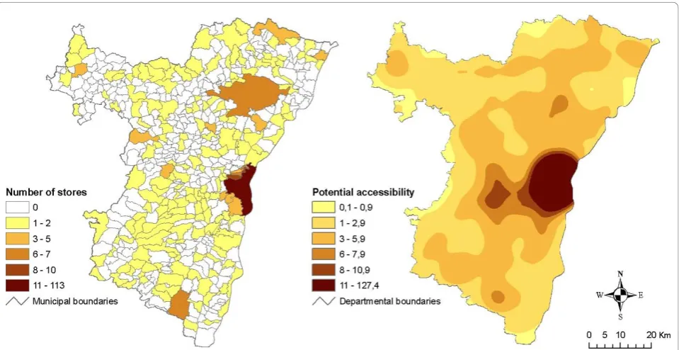
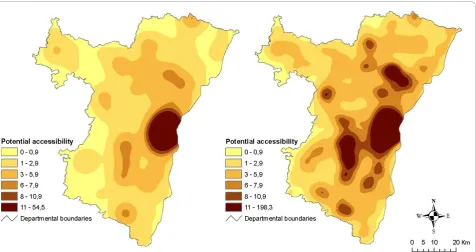
Results are presented on Figures 4 and 5. Producing pseudo-continuous surface maps presents at least two main advantages. First, by getting data that are free from administrative boundaries, it allows approaching a more realistic and precise estimation of accessibility levels. For example, map comparison clearly shows that there are no areas with null accessibility even though facilities are not locally available (i.e. no grocery stores in the municipality) (Figure 4). Second, it proves its use-fulness for emphasising different kinds of retailing stra-tegies. For example, it appears that while accessibility to bakeries is quite good all over the département, hyper/ supermarkets are concentrated in most populated areas (Figure 5).
Comparing count of facilities data and potential accessibility values
In order to compare the output of the first model with original data, potential accessibility values were esti-mated for all municipalities administrative centres (N = 526). Graphical comparisons were conducted between potential accessibility values and number of food outlets and between ranking of municipalities
(first rank for the highest values) according to poten-tial accessibility values and count of facilities data. In both cases, results showed a very high variability in the outputs of the model: except for Strasbourg city, which continued to occupy the first place, ranking of munici-palities appeared completely modified, even for impor-tant cities such as Haguenau and Sélestat (Figure 6). Correlation coefficients were estimated in order to assess the importance of these variations. Because of the extreme skewness of the original data distribution
(see Table 1), we estimated Spearman’s rank
correla-tion coefficients. All associacorrela-tions were statistically sig-nificant at the 0.01 level. Results indicate a poor relationship between the rankings of municipalities for the count of facilities and potential accessibility values (0.342 for grocery stores, 0.355 for hyper/supermarkets and 0.523 for bakeries).
An extended potential model for commuters
The approach developed previously allowed us to esti-mate accessibility levels, but in a very limited and static way. Indeed, so far we did not take into account popula-tion movements across space while the presence of opportunities both in the residential neighbourhood and around activity places (e.g. workplaces) may impact population accessibility levels.
One basic idea is therefore to extend the potential model in order to take account of the case of commu-ters: people have access to opportunities not only in the
area i where they reside, but also in the area kwhere
they work.
In that case, we can estimate a cumulative potential accessibility to a type of servicessuch as:
ΦCiks =ΦCik is , +ΦCik ks , (4)
where ΦCik is
, and ΦCik ks , are respectively the potential
accessibility in i and k for commuters living ini and
working ink.
This first approach does not consider trip lengthdik
betweeni(home) andk(work) and hence that increasing travel time will reduce available time (or time-budget) for a given purpose (e.g. shopping). Because time-budget is not unlimited, if commuting time becomes too long, commuters will not have access to services neither in
inork. It is then necessary to choose a threshold value for trip length beyond which facilities will not be accessi-ble anymore. This thresholdmax(dik)can be defined in
iandkwill be reduced according to a trip length weight-ing function:
( )
max( ) , max( )
d d
d d d
ik ik
ik
ik ik
=⎛ ⎝
⎜ ⎞
⎠
⎟ ≤ (5)
where θ is a parameter reflecting the relationship
between the commuting time or distance and the avail-able time-budget. Standardisation bymax(dik)ensures
that g(dik) ranges from zero whendik equals zero (i.e.
living and working in the same place) to one whendik
equalsmax(dik).
The potential accessibility ΦCiks to a service s for
commuters living in i and working in k can then be
written as:
ΦCiks =(ΦCik is , +ΦCik ks , ) (⋅ −1 (dik)) (6)
where (1 - g(dik)) is the trip length weighting term
which ranges from zero (when no time is available for the given activity, i.e. the travel time is too long) to one (when full time-budget is available, i.e. no travel time).
ΦCiks then theoretically ranges from 0 to 2× ΦCik i s
,
when i and kcoincide (i.e. living and working in the
same place).
Because commuters of a given municipality may have different destinations, we introduce the proportion of commuters for each destination in the previous equation (Equation 6). A global cumulative potential accessibility
for commuters living in a municipality i can then be
written as:
ΦCis ik Φ Φ
i Cik i s
Cik k s
ik k
n
C
C d
= + ⋅ −
=
∑
( , , ) (1 ( ))1
(7)
whereCik is the number of commuters living iniand
working in each destinationkand Ciis the total number
of commuters. ΦCik is
, and ΦCik ks , are estimated using
the potential model (Equation 3).
Estimating potential accessibility for a commuting population
The analysis conducted for the choice of the distance
metric (see section “Methods: choosing the distance
metric”) also allowed us to calibrate theθparameter in the trip length weighting function g(dik) (Equation 5):
the high correlation coefficient value between time and distance led us to conclude that the time-budget should decrease in a linear way as the Euclidean distance
increases and θwas then set to 1. The threshold
dis-tance for which potential accessibility value around home and work reaches zero was defined as the maximum travel distance observed for all commuters (65 km). We estimated commuting-based potential accessibility to hyper/supermarkets, grocery stores and bakeries and compared it to the outputs of the potential model. Models were calibrated using the same para-meters values as previously (see Table 2).
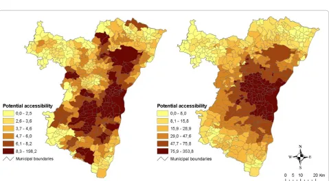
Figure 7Maps of potential accessibility to hyper/supermarkets for residents (left) and commuters (right). These maps make it possible to compare potential accessibility to hyper/supermarkets between residents (left) and commuters (right). Potential accessibility was estimated with an exponential-shaped function and a 19 km span. In the case of commuters, potential accessibility is cumulated in municipalities of both residence and workplace and weighted according to the inverse distance between them and the number of commuters. Class limits are defined according to quantiles.
areas. Map analysis shows that the introduction of jour-ney to work into the model dramatically increases the overall accessibility levels. The impact of Strasbourg city as the biggest employment centre is particularly striking. Indeed in both cases, values seem to follow a clear inverse gradient as the distance to Strasbourg city increases.
Comparing potential accessibility between residents and commuters
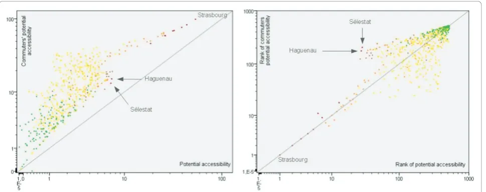
Graphical comparisons reinforce the previous observa-tions of an overall increase in accessibility levels either for supermarkets (Figure 9, left), bakeries (Figure 10, left) or grocery stores (results not shown). In all cases, the increase is high in major urban poles and suburban municipalities. The situation is more contrasted in the case of rural municipalities under urban influence: the increase is very strong for some of them while others have similar levels as rural municipalities out of urban influence. Graphical comparison of ranks confirms that
observation (Figure 9 and 10, right) and Spearman’s
rank correlation coefficients show that the ranking variability is slightly higher for bakeries (0.665) and grocery stores (0.674) than for hyper/supermarkets (0.778). These results can be related to the previous map analysis: distance to urban poles plays a major role in the estimation of accessibility levels. That seems to be especially true in rural remote areas where accessibility levels for both residents and commuters are the lowest.
Discussion
The objective of this study was to propose measures of spatial accessibility to a set of facilities on the regional scale, with the aim of applying the methodology to the field of health behaviours and neighbourhood depriva-tion in future work. For this purpose, we first chose to use a potential accessibility index, and we proposed to improve it by introducing the dynamics of a commuting population.
Data availability
Our developments have mainly been driven by available data. Because commuting data were only available at an aggregated level, it has not been possible to conduct the analysis below the municipality level. Furthermore, as we decided to work with a fairly old database, we were unable to assess data quality (see for example [47], [48] and [49] for methodological discussions on this point). In the present work, we chose to apply our models to three different kinds of food outlets for illustrative pur-poses, and it is important to emphasise here that the method could be applied to any type of facility (e.g. pub-lic services, sport facilities) and using disaggregate data if available.
The potential model: introducing travel behaviour Our work was based on the observation that most stu-dies that attempted to link health behaviours and spatial accessibility used measurements that do not take into account travel behaviour (nearest opportunity, container
index) [11]. We exposed a complete example of applica-tion (including calibraapplica-tion process) of a potential model which is relatively easy to implement and for which only few data are needed for computation. The potential model is very close to the KDE both in a theoretical (gravity-based measure) and practical (spatial smoothing technique) perspective. The main advantage of our method is that every part of the model specification can be controlled, especially the definition of the travel impedance function. This advantage is nevertheless very relative as it is widely accepted that in the case of KDE, compared to the type of function used, the size of the span is much more crucial (i.e. neighbourhood delimita-tion) [13].
The resulting potential accessibility index includes some aspects of travel behaviour and is partly free from administrative boundaries. It may thus provide a more accurate picture of accessibility levels experienced by the population. In our study zone, it appeared for exam-ple that areas with null or very weak accessibility were almost inexistent, reflecting a good global accessibility level to food outlets. These results obviously need to be put in relation with the transport mode chosen and thus with car ownership and transportation possibilities. But
because 85% of the households of the département
owned at least one car (1999 Population Census, INSEE), we hypothesise that our resulting index is valid on this scale of analysis and for this specific study zone.
A classical limitation of such aggregated models is that it assumes that all individuals in a municipality experience the same accessibility level, thus the same
“frictional effect of space”. Indeed, the model was
calibrated using trip length data, assuming that spatial interaction distributions were only due to travel beha-viours, the distance decay being constant for the whole zone studied and the population homogeneous. The model thus did not take into account possible local spa-tial variations of the distance decay which can result either from behavioural discrepancies or from the spa-tial structure effect [50].
Another limitation is that of the lack of data that may have resulted in inaccurate measurements. Results showed that areas with the lowest accessibility levels were mainly distributed near the borders of our study zone (Figure 4). This observation has nevertheless to be interpreted carefully because of the absence of informa-tion about facilities provision outside the département. Indeed it has been shown that edge effects may strongly impact gravity-based accessibility measurements (espe-cially when using large distances) [51].
Integrating the spatial dynamics of a commuting population
considering populations as static“objects” could lead to biased results and may partly explain why published stu-dies on the relationships between individual behaviours and environmental determinants exhibit inconsistent findings [52]. This important result also supports the calls for the developments of new measurements taking into account both residential and non-residential expo-sure [22,53,23,31].
The other strength of this extended model is that it introduces a temporal constraint, although in a very coarse way, through the notion of time-budget. In their study on foodscape exposure, Kestens and collea-gues identified this point as an important one in mea-suring the influence of food stores in a space-time perspective [31].
Several limitations are associated with the develop-ment of our extended potential model. First, the dis-tance and time-budget weighting functions were based on Euclidean distances between municipalities because our analysis showed a very strong correlation between travel-times, network distances and Euclidean distances on the regional scale. Nevertheless, the travel-time model used (see Appendix 1) did not take account of road traffic data, which may strongly impact trip dura-tions (especially during peak hours). Further investiga-tion will therefore be necessary to refine the travel-time model and more generally, to address this question of the time-budget weighting function. It may be indeed relevant to disaggregate our index and to calibrate the weighting functions for different segments of population, e.g. according to median income, age and structures of households [31,54], motorisation rates [55] or travel modes [56].
A second limitation is that the model only considers accessibility for origins (municipality of residence) and destinations (workplace) and thus leads to the underes-timation of potential accessibility levels because facilities present along the daily space-time path are not taken into account. Obviously, the extended model we pro-pose can be refined to include these intervening oppor-tunities. However, we believe with other authors [57,31] that a methodological shift towards individual-based and activity-based models would be necessary to address this question in health studies. In the meantime, given actual data availability, the use of aggregated models still remains necessary when dealing with large study zones.
Conclusions
The aim of this study was to propose measurements of spatial accessibility to a set of facilities on a regional scale. The measurements provided different pictures of accessibility levels. We first applied a potential model which overcomes some of the limitations of more
simple accessibility indices by partly encompassing the multidimensional aspect of the accessibility estimation issue [12]. Then, we proposed an extension to the origi-nal potential model. That allowed us to get very differ-ent results by integrating the dynamics of commuting. Our work supports existing evidence of the importance of the inclusion of specific questions about the location of non-residential activities in health surveys and of the choice of appropriate accessibility indices for analyses dealing with 1) socio-spatial disparities in facilities related to health behaviours and 2) relationships between individual behaviours and accessibility to speci-fic facilities. Such extension of spatial interaction models has potential implications for improving our under-standing of environmental influences on health out-comes on the regional scale, and then for providing relevant information to policy-makers in the field of public health.
Appendix 1 - Building and validating the travel time model
Using a road network database (Georoute 2002, Insti-tut Géographique National, France) and the Network Analyst extension for ArcGIS 9.2 (Environmental Sys-tems Research Institute, Redlands, CA), we estimated network distances and travel times between all the
municipalities in the département. Speed limits were
assigned to each segment of the road network follow-ing previous work of Hilal [58], accordfollow-ing to land-use type (urban vs. rural areas), elevation (hill areas vs. plain areas) and road hierarchy (highways, primary roads, secondary roads).
Appendix 2 - Setting the parameters of the distance weighting function
In a first step, data were log-transformed and linear regression analyses performed for several distance exponents in order to find the best fit (i.e. the minimal standard error of estimate) (Figure 12). Because of our probabilistic approach (probability reaches 1 at null distance), the constant term was not included in the
regression model which then took the form
log ( )Pi = − ⋅ dij where Pi is the probability for
interaction at distance dij.
For non-linear regression analyses, the model was of the form Pi =exp (− ⋅ dij) and the initial parameters used in the iterative process have been set to values relatively close to expected ones (i.e. rounded values of parameters derived from the linear regression analysis).
Acknowledgements
This work is part of the ELIANE (Environmental LInks to physical Activity, Nutrition and hEalth) study. ELIANE is a project supported by the French National Research Agency (Agence Nationale de la Recherche, ANR-07-PNRA-004). JMO is the coordinator of the ELIANE study; CS, BC and CW are the principal investigators in the ELIANE study. The authors would like to thank F. Magnin-Feyssot (Image, Ville, Environnement, Strasbourg, France) for technical assistance.
Author details
1Université de Strasbourg; Image, Ville, Environnement, Strasbourg, France. 2CNRS, ERL 7230, Strasbourg, France.3UMR 8504, CNRS/Université Paris 1,
Géographie-Cités, Paris, France.4UREN, INSERM U557/INRA U1125/CNAM/ Université Paris 13/CRNH Ile-de-France, Bobigny, France.5Université Pierre et
Marie Curie-Paris6; Service de Nutrition, Groupe Hospitalier Pitié-Salpêtrière (AP-HP), Centre de Recherche en Nutrition Humaine Ile-de-France (CRNH IdF), Paris, France.6Lab-Urba, Institut d’Urbanisme de Paris, Université Paris Est-Créteil, France.7Université de Lyon, INSERM/U870 INRA/U1235, CRNH
Rhône-Alpes, Hospices Civils de Lyon, Oullins, France.8INSERM U707, Paris,
France.9Université Pierre et Marie Curie-Paris6, UMR-S 707, Paris, France.
Authors’contributions
PS and AB conceived and designed the study. PS performed analysis and interpretation of data, parts of the programming and drafted the
manuscript. AB performed the main part of the programming and helped to draft the manuscript. JMO, HC, CS, BC, RC, DB, and CW participated in the critical revision of manuscript. All authors have read and approved the final manuscript.
Competing interests
The authors declare that they have no competing interests.
Received: 30 September 2010 Accepted: 10 January 2011 Published: 10 January 2011
References
1. Ingram D:The concept of accessibility: A search for an operational form.
Regional Studies1971,5:101-107.
2. Vickerman RW:Accessibility, attraction, and potential: a review of some concepts and their use in determining mobility.Environment and Planning A1974,6:675-691.
3. Morris JM, Dumble PL, Wigan MR:Accessibility indicators for transport planning.Transportation Research Part A: General1979,13:91-109. 4. Pirie GH:Measuring accessibility: a review and proposal.Environment and
Planning A1979,11:299-312.
5. Koenig JG:Indicators of urban accessibility: Theory and application.
Transportation1980,9:145-172.
6. Handy SL, Niemeier DA:Measuring accessibility: an exploration of issues and alternatives.Environment and Planning A1997,29:1175-1194. 7. Geurs KT, van Wee B:Accessibility evaluation of land-use and transport
strategies: review and research directions.Journal of Transport Geography 2004,12:127-140.
8. Brownson RC, Hoehner CM, Day K, Forsyth A, Sallis JF:Measuring the Built Environment for Physical Activity: State of the Science.American Journal of Preventive Medicine2009,36:S99-S123.
9. Lytle LA:Measuring the Food Environment: State of the Science.
American Journal of Preventive Medicine2009,36:S134-S144. Figure 11 Differences of travel times between model and
operators according to trip length. This graph shows differences between travel times estimated by our model and on-line operators. Difference in minutes is plotted for each pair of municipalities exchanging commuters according to trip duration.
10. Gordon-Larsen P, Nelson MC, Page P, Popkin BM:Inequality in the Built Environment Underlies Key Health Disparities in Physical Activity and Obesity.Pediatrics2006,117:417-424.
11. Charreire H, Casey R, Salze P, Simon C, Chaix B, Banos A, Badariotti D, Weber C, Oppert JM:Measuring the Food Environment Using Geographical Information Systems: A Methodological Review.Public Health Nutrition2010, 1-13.
12. Talen E, Anselin L:Assessing spatial equity: an evaluation of measures of accessibility to public playgrounds.Environment and Planning A1998,
30:595-613.
13. Silverman B:Density estimation for statistics and data analysisLondon: Chapman and Hall; 1986.
14. Luo W, Qi Y:An enhanced two-step floating catchment area (E2SFCA) method for measuring spatial accessibility to primary care physicians.
Health & Place2009,15:1100-1107.
15. Guagliardo M:Spatial accessibility of primary care: concepts, methods and challenges.International Journal of Health Geographics2004,3:3. 16. Yang D, Goerge R, Mullner R:Comparing GIS-Based Methods of
Measuring Spatial Accessibility to Health Services.Journal of Medical Systems2006,30:23-32.
17. Diez Roux AV, Evenson KR, McGinn AP, Brown DG, Moore LV, Brines S, Jacobs DR:Availability of Recreational Resources and Physical Activity in Adults.American Journal of Public Health2007,97:493-499.
18. Moore LV, Diez Roux AV, Brines S:Comparing Perception-Based and Geographic Information System (GIS)-Based Characterizations of the Local Food Environment.Journal of Urban Health2008,
85:206-216.
19. Moore LV, Diez Roux AV, Nettleton JA, Jacobs DR:Associations of the Local Food Environment with Diet Quality–A Comparison of Assessments based on Surveys and Geographic Information Systems.
American Journal of Epidemiology2008,167:917-924.
20. Riva M, Apparicio P, Gauvin L, Brodeur J:Establishing the soundness of administrative spatial units for operationalising the active living potential of residential environments: an exemplar for designing optimal zones.International Journal of Health Geographics2008,7:43. 21. Chaix B, Merlo J, Evans D, Leal C, Havard S:Neighbourhoods in
eco-epidemiologic research: Delimiting personal exposure areas. A response to Riva, Gauvin, Apparicio and Brodeur.Social Science & Medicine2009,
69:1306-1310.
22. Ball K, Timperio A, Crawford D:Understanding environmental influences on nutrition and physical activity behaviours: where should we look and what should we count?International Journal of Behavioral Nutrition and Physical Activity2006,3:33.
23. Chaix B:Geographic Life Environments and Coronary Heart Disease: A Literature Review, Theoretical Contributions, Methodological Updates, and a Research Agenda.Annual Review of Public Health2009,30:81-105. 24. Frank LD, Glanz K, McCarron M, Sallis JF, Saelens BE, Chapman J:The
Spatial Distribution of Food Outlet Type and Quality around Schools in Differing Built Environment and Demographic Contexts.Berkeley Planning Journal2006,19:79-95.
25. Pearce J, Blakely T, Witten K, Bartie P:Neighborhood Deprivation and Access to Fast-Food Retailing: A National Study.American Journal of Preventive Medicine2007,32:375-382.
26. Zenk SN, Powell LM:US secondary schools and food outlets.Health & Place2008,14:336-346.
27. Kestens Y, Daniel M:Social Inequalities in Food Exposure Around Schools in an Urban Area.American Journal of Preventive Medicine2010,39:33-40. 28. Jeffery R, Baxter J, McGuire M, Linde J:Are fast food restaurants an
environmental risk factor for obesity?International Journal of Behavioral Nutrition and Physical Activity2006,3:2.
29. Kwan MP:Space-Time and Integral Measures of Individual Accessibility: A Comparative Analysis Using a Point-based Framework.Geographical Analysis1998,30:191-216.
30. Kwan MP:Gender and individual access to urban opportunities: a study using space-time measures.Professional Geographer1999,51:210-227. 31. Kestens Y, Lebel A, Daniel M, Thériault M, Pampalon R:Using experienced
activity spaces to measure foodscape exposure.Health & Place2010,
16:1094-1103.
32. Hansen WG:How Accessibility Shapes Land Use.Journal of the American Institute of Planners1959,25:73.
33. Salze P, Badariotti D, Banos A, Charreire H, Oppert JM, Casey R, Simon C, Chaix B, Weber C:Entre dasymétrique et choroplète: typologie de l’espace adaptée à l’étude des relations entre santé et environnement.
InActes des Neuvièmes Rencontres de Théo Quant: 4-6 March 2009; Besançon, FranceEdited by: Foltête J-C .
34. Eymard I:De la grande surface au marché: à chacun ses habitudes.Insee Première1999,636.
35. Ravenstein EG:The Laws of Migration.Journal of the Statistical Society of London1885,48:167-235.
36. Reilly WJ:The law of retail gravitationNew York; 1931.
37. Stewart JQ:An Inverse Distance Variation For Certain Social Influences.
Science1941,93:89-90.
38. Pooler J:Measuring geographical accessibility: a review of current approaches and problems in the use of population potentials.Geoforum 1987,18:269-289.
39. Liu S, Zhu X:Accessibility Analyst: an integrated GIS tool for accessibility analysis in urban transportation planning.Environment and Planning B: Planning and Design2004,31:105-124.
40. Apparicio P, Abdelmajid M, Riva M, Shearmur R:Comparing alternative approaches to measuring the geographical accessibility of urban health services: Distance types and aggregation-error issues.International Journal of Health Geographics2008,7:7.
41. Taylor P:Distance decay in spatial interactions.Concepts and Techniques in Modern Geography1975,N°2.
42. Echenique M, Crowther D, Lindsay W:A spatial model of urban stock and activity.Regional Studies1969,3:281-312.
43. MTARTS:Metropolitan Toronto And Region Transportation StudyProvince of Ontario, Toronto; 1966.
44. Grasland C, Mathian H, Vincent J:Multiscalar analysis and map generalisation of discrete social phenomena: Statistical problems and political consequences.Statistical Journal of the United Nations Economic Commission for Europe2000,17:157-188.
45. Betz D:XLISP: An experimental object-oriented programming language.
1988.
46. Tierney L:Xlisp-Stat: A Statistical Environment Based on the XLISP Language.1989.
47. Paquet C, Daniel M, Kestens Y, Leger K, Gauvin L:Field validation of listings of food stores and commercial physical activity establishments from secondary data.International Journal of Behavioral Nutrition and Physical Activity2008,5:58.
48. Cummins S, Macintyre S:Are secondary data sources on the
neighbourhood food environment accurate? Case-study in Glasgow, UK.
Preventive Medicine2009,49:527-528.
49. Lake AA, Burgoine T, Greenhalgh F, Stamp E, Tyrrell R:The foodscape: Classification and field validation of secondary data sources.Health & Place2010,16:666-673.
50. Fotheringham AS:Spatial Structure and Distance-Decay Parameters.Annals of the Association of American Geographers 1981,71:425-436.
51. Van Meter EM, Lawson AB, Colabianchi N, Nichols M, Hibbert J, Porter DE, Liese AD:An evaluation of edge effects in nutritional accessibility and availability measures: a simulation study.International Journal of Health Geographics2010,9:40.
52. Wendel-Vos W, Droomers M, Kremers S, Brug J, Lenthe FV:Potential environmental determinants of physical activity in adults: a systematic review.Obesity Reviews2007,8:425-440.
53. Inagami S, Cohen DA, Finch BK:Non-residential neighborhood exposures suppress neighborhood effects on self-rated health.Social Science & Medicine2007,65:1779-1791.
54. Páez A, Gertes Mercado R, Farber S, Morency C, Roorda M:Relative Accessibility Deprivation Indicators for Urban Settings: Definitions and Application to Food Deserts in Montreal.Urban Studies2010,
47:1415-1438.
56. Shen Q:Spatial technologies, accessibility, and the social construction of urban space.Computers, Environment and Urban Systems1998,22:447-464. 57. Saarloos D, Kim J, Timmermans H:The Built Environment and Health:
Introducing Individual Space-Time Behavior.International Journal of Environmental Research and Public Health2009,6:1724-1743.
58. Hilal M:Temps d’accès aux équipements au sein des bassins de vie des bourgs et petites villes.Economie et statistiques2007,402:41-56.
doi:10.1186/1476-072X-10-2
Cite this article as:Salzeet al.:Estimating spatial accessibility to facilities on the regional scale: an extended commuting-based interaction potential model.International Journal of Health Geographics 201110:2.
Submit your next manuscript to BioMed Central and take full advantage of:
• Convenient online submission
• Thorough peer review
• No space constraints or color figure charges
• Immediate publication on acceptance
• Inclusion in PubMed, CAS, Scopus and Google Scholar
• Research which is freely available for redistribution