Statistical Model Checking of Web Services

(1)

PhD Dissertation

International Doctorate School in Information and Communication Technologies

DIT - University of Trento

S

   

W



S



Stefano Schivo

Advisor:

Prof. Paola Quaglia

Universit`a degli Studi di Trento

(2)

(3)

Imagination, not intelligence, made us human.

(4)

(5)

Abstract

In recent years, the increasing interest on service-oriented paradigm has given rise to a series of supporting tools and languages. In particular, COWS (Calculus for Orchestration of Web Services) has been attracting the attention of part of the scientific community for its peculiar effort in formalising the semantics of the de facto standard Web Services orchestration language WS-BPEL. The purpose of the present work is to provide the tools for representing and evaluat-ing the performance of Web Services modelled through COWS. In order to do this, a stochastic version of COWS is proposed: such a language allows us to describe the performance of the modelled systems and thus to represent Web Services both from the qualitative and quantitative points of view. In particular, we provide COWS with an extension which maintains the polyadic matching mechanism: this way, the language will still provide the capability to explicitly model the use of session identifiers. The resultingSis then equipped with a software tool which allows us to effectively perform model checking without incurring into the problem of state-space explosion, which would otherwise thwart the computation efforts even when checking relatively small models. In order to obtain this result, the proposed tool relies on the statistical analysis of simulation traces, which allows us to deal with large state-spaces without the actual need to completely explore them. Such an improvement in model checking performances comes at the price of accuracy in the answers provided: for this reason, users can trade-off speed against accuracy by modifying a series of parameters. In order to assess the efficiency of the proposed technique, our tool is compared with a number of existing model checking softwares.

Keywords

(6)

(7)

List of Tables

2.1 BNF grammar of the Continuous Stochastic Logic (CSL). . . 9

2.2 Semantics of CSL formulas. . . 9

3.1 The grammar of S. . . 12

3.2 Semantics for S(Part 1). . . 14

3.3 Semantics for S(Part 2). . . 15

3.4 Definition of functionsopandops. . . 16

3.5 Derivation of the example showing the application of ruleopen. . . 16

3.6 Definition of the matching functionM. . . 17

3.7 Definition of functioninv. . . 21

3.8 Definition of functionreq. . . 24

3.9 Definition of functionbms. . . 24

3.10 Definition of functionaR. . . 24

3.11 Definition of functionsumRates. . . 25

3.12 Definition of functionaInv. . . 25

3.13 Structural congruence rules for S. . . 27

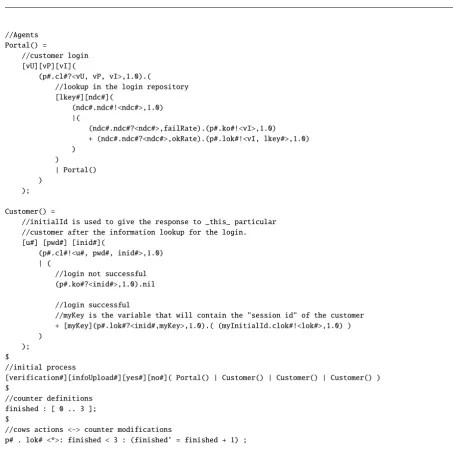
4.1 An example input for S amc. . . 44

4.2 Example CSL input formulas for S amc. . . 44

5.1 The problem of 6 dining philosophers modelled with S. . . 52

5.2 The problem of the sleeping barber with 2 chairs and 3 customers. . . 54

5.3 Computational time results for the model checking of Formula 5.1. . . 57

5.7 Values of formulaP₌_?[trueU[0,20] _cut_> ₂_{]. . . .} ₆₁

5.8 Results of the model checking on the SENSORIA finance case study. . . 63

A.1 COWS structural congruence. . . 68

A.2 COWS operational semantics. . . 69

A.3 Encoding functions from polyadic COWS to monadic COWS (part 1). . . 71

(10)

A.7 Services resulting from the encoding of proposed example (Part 2). . . 78

A.8 Services resulting from the encoding of proposed example (Part 3). . . 79

B.1 Smodel of the financial case study. . . 85

(11)

List of Figures

4.1 Hypothesis testing: ideal case. . . 33

4.2 Hypothesis testing: real case. . . 34

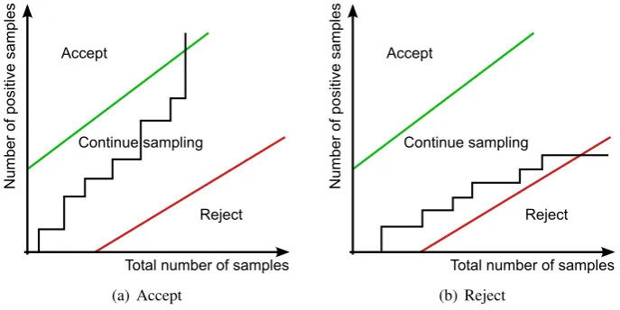
4.3 Two possible execution paths of the SPRT algorithm. . . 35

4.4 Choosing the next transition step when generating a simulation trace. . . 45

4.5 The user interfaces provided by the S amc tool. . . 47

4.6 Checking the example model. . . 48

5.1 An example configuration of the dining philosophers. . . 50

5.2 Graph comparing the performances of the tools S lts and S amc. . . . 57

(12)

(13)

Chapter 1

Introduction

1.1

The Context

In recent years the world of Web Services has been attracting the interest of part of the scientific community because of the success of the service oriented interaction paradigm on which it is based. A number of existing formal languages have been successfully applied for modelling Web Services [10, 7, 34], while some others have been proposed specifically for this aim [9, 8, 17]. Among these formalisms, COWS (Calculus for Orchestration of Web Services [30]) has been recently attracting the attention of a part of the scientific community for its peculiar effort in formalising the semantics of the de facto standard Web Services orchestration language WS-BPEL [6]. The calculus allows us to model different and typical aspects of services and Web Services technologies, such as multiple start activities, receive conflicts, routing of correlated messages, service instances and interactions among them. COWS can express the most common workflow patterns and has been shown to encode other process and orchestration languages [30]. One of the peculiarities of COWS is its matching mechanism, through which the concept of session identifier is modelled, effectively providing a way to correlate interactions belonging to the same session. We will now present a brief example illustrating the polyadic matching communication paradigm as defined in COWS. Consider the following service (i.e., COWS process) definition, in which sub-services have been labelled for convenience:

S = p!hm,ni

| {z } s1

| p?hx,yi.s0₂ | {z }

s2

| p?hx,ni.s0₃ | {z }

s3

(14)

the same session). The communication paradigm defined in COWS is based on the idea ofbest matching, which means that any given sending action (which will be called from now oninvoke action) can communicate only with one of the receiving actions (namedrequest actions) whose parameters match the best way with the ones being sent. This means that the number of variable substitutions generated by a communication involving invoke action p!hm,nihas to be minimal w.r.t. all request actions in the whole service. In our case this translates into the possibility to haveonly onecommunication happening inS: the one involving servicess1ands3. In fact, the communication between s1 ands2 would generate two substitutions (replacing xwithmandy withn), while the communication betweens1and s3generates only one substitution (replacing xwithmand matchingnwithn). Thus, we can think of services s1and s3 as belonging to the same session, identified by namen.

As a final remark, notice that if a third request action in the form p?hn,yiwould have been available, it would not have been able to participate to the communication either, because it requires the name n to be in the first position of the tuple, while service s1 offers m as first parameter.

1.2

The Problem

The purpose of this thesis is to provide the tools for representing and evaluating the performance of Web Services modelled through COWS. In order to do this, a stochastic version of COWS is required: such a language would allow dealing with the performance of the modelled systems, thus fastening the analysis of Web Services both from the qualitative and quantitative points of view.

Actually, a stochastic extension of COWS has already been proposed in [35], but the version presented there is based on a monadic fragment of the language (i.e., communications allow exchanging only one name at a time). One of the objectives of our work is to provide COWS with an extension which keeps the polyadic matching mechanism; this will in turn allow us to maintaining the capability to explicitly model the use of session identifiers. Moreover, while we are confident that a monadic version of COWS would maintain the same expressivity as the original calculus (in Appendix A we provide an encoding from COWS to its monadic fragment), the same relation between a monadic stochastic extension of COWS and its polyadic counterpart would be troublesome to be proven. Intuitively, at a certain point of the proof a single stochastic execution step (in the polyadic calculus) should be matched with a series of stochastic execution steps (in the monadic calculus). However, as a sequence of exponentially distributed delays is not exponentially distributed itself, the rates of the two cases would not correspond, and thus the correspondence could not be accomplished.

(15)

CHAPTER 1. INTRODUCTION 1.3. THE SOLUTION

model checking methods to obtain the required performance measures. However, a common problem which needs to be faced when generating a transition system of a process calculus term is the so-called state-space explosion. This problem comes from the fact that the composition of xparallel processes each withydifferent states in its transition system gives rise to a transition system with at mostyx_{states, thus requiring (as an upper bound) exponential time and resources} to be computed. A solution often applied is to generate the state-spaces of the subprocesses in isolation, and then, taking advantage of the characteristics of some compact representation (e.g., in the case of stochastic calculi, Multi Terminal Binary Decision Diagrams [15] are sometimes employed), merge the resulting transition systems, obtaining a description of the whole state-space of the starting process using less-than-exponential time and memory resources. However, such compositional approach cannot be applied in our case, because the stochastic calculus presented in this thesis inherits the matching communication paradigm directly from COWS. As illustrated before, this paradigm requires the knowledge of the complete process in order to compute any transition. There are however other ways of mitigating the state-space explosion problem in the case of our calculus: see for example the S lts tool by Igor Cappello [11, 12], in which the application of a congruence notion largely improves the tractability of the problem. An objective of this work is to explore the possibility to apply a different approach to the model checking of stochastic COWS models.

1.3

The Solution

As anticipated in Section 1.2, our work consists in the design of a stochastic extension of COWS which maintains the polyadic communication paradigm peculiar to the calculus. The resulting Sis a stochastic calculus whose syntax adheres to the original version of COWS, to which only minor adjustments are made in order not to obtain infinitely branching transition systems from Smodels. This eventuality would in fact bar the possibility to obtain proper CTMCs from S models. The most important extension introduced in S is the association of a stochastic rate to each basic action of the language: these rates are the parameters of exponentially distributed random variables each describing the duration of the associated action. The stochastic operational semantics of Sallows to obtain the possible actions available to a starting service, while the actual rates of such actions are computed through a formula which takes into account the communication capabilities of all entities involved in each interaction. Even if communication actions are binary operations, involving only two distinct services, other services can be indirectly involved into the rate computation: these are the services offering communication endpoints defined to bein competition with the ones actually communicating. Briefly explained, a services1competes with services2for a particular communication ifs1can take the place of s2 in the same communication. Notice that this way of computing transition rates is directly based on COWS communication paradigm, thus allowing us to keep intact as much as possible the foundational ideas of COWS.

(16)

which does not require to compute the whole state space of a S model; instead, it works through a direct simulation-based approach inspired by [40] and [19]. What we do in practice is to generate a number of simulation traces starting from a given Smodel, and from these we obtain the required performance measures through statistical reasoning. In particular, the traces are generated by iteratively applying the stochastic operational semantics to the starting model, while the number of simulation traces needed to obtain a desired confidence is derived from the user-defined error thresholds. These thresholds can be tuned via a trade-offbetween execution time and approximation, thus allowing to obtain more precise results when time is not an (important) issue, while allowing to get likely estimations after a few minutes (or even seconds) of computation.

1.4

Innovative Aspects

The introduction of Sallows to describe the quantitative aspects of Web Services, while still maintaining the capabilities provided by the polyadic communication paradigm peculiar to COWS. The proposed tool, providing a way to perform model checking on S models, and thus derive performance measures on the modelled Web Services, allows to fully exploit the potentials of the language without having to deal with complete state-space generation (and thus with the problem of state-space explosion). The approach used in our tool turns out to be even more useful than the generation of the whole transition system of a model (from which a CTMC is then to be derived) when the number of parallel components contained the S model at hand reaches high values. In practice, this allows us to extend the number of tractable Smodels, which has already been successfully increased by the S amc tool.

The performance of the proposed tool is compared with other existing model checking tools. In order to have a common field of comparison between our tool and existing model checking tools, we first generate a CTMC from the S model at hand, and then give it as input to other model checking tools. As CTMCs are the favored input language for a substantial number of model checking tools, this choice enables us to compare our work with some of the most widespread tools. This comparison comes at the price of running into the state-space explosion problem while generating the CTMC, even if with greatly reduced effects, thanks to S lts. This problem considerably increases the combined model checking time. However, the step of CTMC generation has to be taken into account when computing the total model checking time, as the comparisons we make are about model checking Smodels.

1.5

Overview of the thesis

(17)

CHAPTER 1. INTRODUCTION 1.5. OVERVIEW OF THE THESIS

(18)

(19)

Chapter 2

State of the art

In this chapter we will present two of the main languages for service-oriented modelling: WS-BPEL [6] and BPMN [33]. Taking hint from the lack of formal definition in these languages, we will show an attempt to remedy to their shortcomings with the process algebra COWS [30]. Furthermore, we will present a series of extensions to the COWS language, together with a tool for the qualitative assessment of COWS models. We will then proceed with the presentation of some methods and tools for testing quantitative properties of systems. The quantitative testing of a system comprises the evaluation of the performances of the system after having assigned numerical duration to the actions represented by a model. The typical quantitative reasoning tools are based on continuous time Markov chains (CTMC, [26]), a mathematical formalism used to represent systems with stochastic behaviour.

2.1

Web service modelling languages

2.1.1 WS-BPEL

(20)

2.1.2 BPMN

BPMN [33] (Business Process Modelling Notation) is a graphical representation for web ser-vices orchestrations, whose purpose is to allow business-process technicians to easily model web service interactions. The notation is equipped with an intuitive set of symbols which represent WS-BPEL functionalities, but it suffers from lack of ontological completeness and clarity [37]. Moreover, it has been recently pointed out that BPMN and WS-BPEL suffer from conceptual mismatch in the representation of some control flow patterns [38]. Concluding, we do not consider the language mature enough to come out useful in real business process modelling, and thus it cannot be safely used as an effective visual representation of WS-BPEL models.

2.1.3 COWS

COWS is a process calculus first introduced in [30] as an evolution of-[31], with the aim to model service-oriented orchestrations. The language is particularly interesting because its predecessor was created with the purpose to give a formal semantics to WS-BPEL (through the translation presented in [31]), and more work is being carried out with the aim to obtain a complete mapping of WS-BPEL into COWS [32]. The interest roused by COWS is also due to its mainly web services-oriented primitives, since many of its basic constructs come from the SOC world.

2.2

Stochastic modelling

2.2.1 Continuous-time Markov chains

Continuous-time Markov chains (CTMCs [26]) are a widely used formalism generated by the semantics of SPAs such as Stochastic COWS, and are at the basis of performance evaluation in many different areas.

Definition 1. A continuous time Markov chain (CTMC) is a pairC=(S,R)where

• S is a countable set of states

• R:S ×S → _>0such thatPs0_∈SR(s,s0)converges is arate matrix

Taken a CTMCC=(S,R), theexit ratefor state s∈S is E(s)=X

s0_∈S

R(s,s0)<∞

We can compute the probability to move from state s ∈ S to a state s0 ∈ S (such that R(s,s0)> 0) beforettime units using the exponential distribution function:

(21)

CHAPTER 2. STATE OF THE ART 2.3. QUANTITATIVE MODEL CHECKING

whereλ= R(s,s0).

The probability that the transitions → s0is chosen between all transitions exiting from s(that is, the probability that the delay for going fromstos0“finishes before” any other delay of going fromsto another states00 _, s0) is

P[s→ s0]= R(s,s 0₎

E(s)

2.3

Quantitative model checking

Probabilistic model checking of a stochastic model is the technique which allows us to measure the quantitative aspects of the model through probabilistic reasoning. In particular, if the model can be represented as a CTMC, a common probabilistic model checking approach allows us to define some properties against which the model is to be checked. Such properties are defined using a specification language suitable to the model: for example, in the case of CTMC, a suggested property specification language is CSL (Continuous Stochastic Logic, [5]), whose BNF grammar is presented in Table 2.1.

(state formula) Φ ::= true | false | a | ¬Φ | Φ∧Φ | Φ∨Φ | S./θ[Φ] | P./θ[ϕ] | S₌?[Φ] | P=?[ϕ]

(path formula) ϕ ::= XΦ | ΦUΦ | ΦU[tmin,tmax]Φ

Table 2.1: BNF grammar of the Continuous Stochastic Logic (CSL). Here, a is an atomic formula,

θ∈[0,1],./∈ {<,₆, >,_>}andtmin,tmax∈.

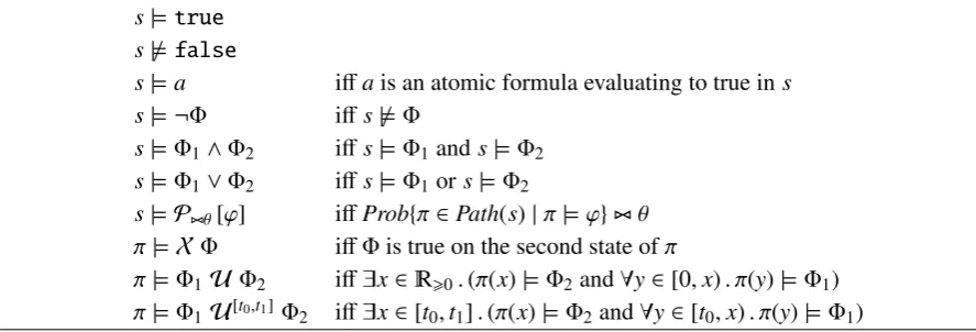
The semantics of CSL formulas defines how to verify if a particular state s of the CTMC satisfies a CSL state formulaΦ(writtens|= Φ), and is presented in Table 2.2.

s|=true s6|=false

s|=a iffais an atomic formula evaluating to true ins

s|=¬Φ iffs6|= Φ

s|= Φ₁∧Φ₂ iffs|= Φ₁ands|= Φ₂

s|= Φ1∨Φ2 iffs|= Φ1ors|= Φ2

s|=P./θ[ϕ] iffProb{π∈Path(s)|π|=ϕ}./ θ

π|=XΦ iff Φis true on the second state ofπ

π|= Φ1UΦ2 iff∃x∈>0.(π(x)|= Φ2and∀y∈[0,x). π(y)|= Φ1)

π|= Φ₁U[t0,t1] Φ

2 iff∃x∈[t0,t1].(π(x)|= Φ2and∀y∈[t0,x). π(y)|= Φ1)

(22)

(23)

Chapter 3

S



In this chapter we introduce a stochastic extension of COWS, which will be used in the follow-ing as a base for the statistical model checkfollow-ing of Web Services.

The objective of the stochastic extension is to provide the modelling language COWS with a way to represent also quantitative aspects of Web Services, allowing thus to test their perfor-mance and draw inferences on the efficiency of the modelled entities. In order to do this, the base actions of COWS are enriched with a real value, called rate. Such rates are the parameters of exponentially distributed random variables, which model the duration of the corresponding actions.

As we will see, maintaining the matching mechanism peculiar to COWS will be one of the major challenges in adding stochastic capabilities to the language. This happens because we want to make sure that the communication capabilities of individual services (which in COWS are called “services”) are taken into account when computing the rate of an interaction happening inside a composite service.

3.1

Stochastic semantics for COWS

S services are represented as basic activities composed following the grammar shown in Table 3.1, and based on three countable and disjoint sets ofentities: the set of namesN (with metavariablesm,n,o,p,m0,n0,o0,p0), the set of variablesV(with metavariablesx,y,z,x0,y0,z0) and the set of killer labelsK (with metavariables k,k0). Adhering to the conventions adopted in [30], we shall indicate elements ofN ∪ Vwithu,v,w,u0,v0,w0, and elements ofN ∪ V ∪ K

withd,d0. Notice that, differently from the original version of the language, we do not consider the class of “values” in our grammar, as in our case the management of values and expressions would lead to a more complicated operational semantics without adding significance to the stochastic extension.

(24)

we set that a sequence of delimiters can be rewritten as a delimiter for a tuple of entities: i.e.,

[d1][d2]. . .[dj]s = [˜d]s, where ˜d = hd1,d2, . . .dji. Furthermore, we define the (possibly

empty) delimiter tuple as

˜

t::=n˜ | ε

The writing of the form [˜t]sin the residual services of rulecom(cfr. Table 3.2) will be intended as salone if ˜t = ε, and as [˜n]sif ˜t = n˜. Finally, the substitution of entities in tuples is written

˜

w{n/_x_}_{, and defined as the substitution of all occurrences of}_x_{in ˜}_w_with_n_.

s ::= (u.u!˜u, δ) | g | s|s | {|s|} | (kill(k), λ) | [d]s | S(m1, . . . ,mj)

g ::= 0 | (p.o?˜u, γ).s | g+g

Table 3.1: The grammar of S.

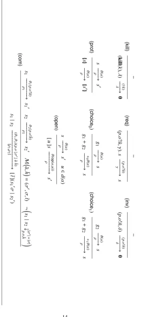
Following a common approach in stochastic extensions [23, 36, 35], we associate a stochas-tic delay to each basic action of the language. These delays are determined via exponentially distributed random variables, the rates of which are included in the syntax of basic actions. The three basic actions are invoke (u.u0!˜u, δ), request (p.o?˜u, γ) and kill (kill(k), λ), and represent re-spectively the capacity to send an output tuple ˜uthrough endpointu.u0, receive an input on tuple

˜

uthrough endpoint p, and request the termination of all (unprotected) services under the scope of killer label k; the rates of these activities are respectively δ, γ and λ. The basic activities are assembled through the classical combinators of parallel composition s | s, guarded choice g+ g(the classical nondeterministic choice, in which each service has to start with a request action) and service identifierS(m1, . . . ,mj). The last allows to express recursive behaviour and is associated to a corresponding service definition of the formS(n1, . . . ,nj)= s included in the model definition. The employment ofdelimiters[d]sallows to define the scope of entities, and thus to delimit the extent of variable substitution, the validity of names and the limits for service termination. An entity under the scope of a delimiter is said to beboundby that delimiter. For example, in the service S = [x]((p.o?x, γ).(p.o!x, δ)) the variable x is bound by the delimiter [x], while the name p is not bound. A S service S is termed closed if every entity ap-pearing in Pis bound by a delimiter. In order to delimit the effects of service termination, in addition to killing label termination and adhering to the features present in COWS, we provide the protection construct{| |} with the same semantics as in the original version of the language.

(25)

CHAPTER 3. SCOWS 3.1. STOCHASTIC SEMANTICS FOR COWS

the starting service and kept valid through the use of functions s dec and l dec in ruleserid(cfr.

Tables 3.2 and 3.3). These functions are directly drawn from [35] and decorate bound names respectively in the transition label and in the residual service by adding to each entity a finite number of zeroes as superscript.

The form of a generic transition obtained from the application of the operational semantics

rules of Tables 3.2 and 3.3 to a (closed) Sservice iss

ϑ(α)

−−−−→_ρ s0. Here,αis the action label;

ρis the rate associated to the basic action, or a pair formed by the rates of the two interacting services if the action is a communication; andϑis a string of “+0” and “+1” created through the application of ruleschoice0 and choice1. The last approach is drawn from the one presented in [35] in order to distinguish between transitions which would otherwise be identical. As an example, consider the following service:

S =(p.o!n, δ)|(p.o?n, γ).0+ (p.o?n, γ).0 FromS, two transitions lead to the same residual:

S −−−−−−−−−−−+0(p.ob∅cn n→)

[γ, δ] 0|0 and S

+1(p.ob∅cn n)

−−−−−−−−−−−→

[γ, δ] 0|0.

Notice that, if we had not established a way to distinguish between the two transitions, the total rate of the transitions labelled withp.ob∅cn nexiting fromS would have been computed taking into account only one transition, and not two, thus leading to an inconsistent representation of the model.

In addition to the metavariable conventions mentioned before, in the operational semantics rules we will usea,bto range overu,u0,(u),(u0) (i.e. possiblyboundinput entities) andh,ito range overm,n,(m),(n) (i.e. possibly bound output names). In operational semantics labels, we call an entity “bound” if it falls under the scope of a delimiter in the service on which the

semantics rules are being applied. For example, in the transition [x](p.o?x, γ).s−−−−−−−(p.o_γ?(x))→ swe use (x) in the label to state that the scope of xhas been opened (by applying rule open), and thus thatxis bound in the starting service.

Finally, in order not to obtain infinitely branching transition systems, we have to avoid the use of a congruence relation within the operational semantics rules. For this reason we deal with opening and closing of scopes with specific semantic rules: open, com and delcl. Rule open

uses the functionop(see Table 3.4) to actually modify transition labels, opening the scope of bound entities, and signaling their bound status in the resulting transition label. Rulescomand

delcl handle the closing of scopes for names sent in a communication.

Notice that the given definition for rule openallows to extrude the scope of names for all three communicating labels. This allows us to take into account also the case in which the scope of the input variable of the request action contains the scope of the output name from the invoke action, which in turn containsboth communicating services. As an example, consider the following service:

(26)

(27)

CHAPTER 3. SCOWS 3.1. STOCHASTIC SEMANTICS FOR COWS ( par conf ) s1 ϑ ( p . o b σ c ˜ a

˜h)

−− −− −− −− −− −→ ρ s1 0 ¬ s2 ↓ #( ˜ a ,

˜h)

p . o , ˜h s1 | s2 ϑ ( p . o b σ c ˜ a

˜h)

−− −− −− −− −− −→ ρ s1 0 | s2 ( par pass ) s1 ϑ ( α ) −− −− → ρ s1 0 α , p . o b σ c ˜a ˜h α , † k s1 | s2 ϑ ( α ) −− −− → ρ s1 0 | s2 ( par kill ) s1 ϑ ( † k ) −− −− −→ _ρ s1 0 s1 | s2 ϑ ( † k ) −− −− −→ _ρ s1 0 | halt ( s2 ) ( del pass ) s ϑ ( α ) −− −− → ρ s 0 d < d ( α ) s ↓kill ⇒ ( α = † or α = † k ) [ d ] s ϑ ( α ) −− −− → ρ [ d ] s 0 ( del cl ) s ϑ ( p . o b σ U { ( n ) / x }c ˜ a

˜h)

−− −− −− −− −− −− −− −− −− → ρ s 0 [ x ] s ϑ ( p . o b σ c ˜ a

˜h)

−− −− −− −− −− −→ ρ [ n ] s

0n{

/ x } ( del sub ) s ϑ ( p . o b σ U { n / x }c ˜ a

˜h)

−− −− −− −− −− −− −− −− −→ ρ s 0 [ x ] s ϑ ( p . o b σ c ˜ a

˜h)

−− −− −− −− −− −→ ρ s

0n{

/ x } ( del kill ) s ϑ ( † k ) −− −− −→ _ρ s 0 [ k ] s ϑ ( † ) −− −− → ρ [ k ] s 0 ( ser id ) s { m1 ,. .. ,

(28)

op(p.o!˜h,n) = p.o!˜h0where ˜h0 =h˜{(n)/_n_}

op(p.o?ã,x) = p.o?ã0where ã0=a˜{(x)/_x_}

op(p.obσca˜ h,˜ n) = p.obop_s(σ,n)ca˜ h˜0where ˜h0=h˜{(n)/n}

ops(∅,n) = ∅

ops({n/x} ]σ,m) =       

{(n)/_x_{} ]}_op

s(σ,m) ifn=m

{n/_x_{} ]}_op

s(σ,m) ifn,m

Table 3.4: Definition of functionsopandop_s used for the opening of input, output and communication

labels.

Here, the scope ofncan be correctly extended via the application of ruleopen, generating the transition s−−−−−−−−−−−→ϑ(p.ob∅cx(n))

[γ, δ1] [n] (0

|0|(q.m!n, δ2)). The derivation of such transition is shown in Table 3.5, where the application of ruleopenis marked by (∗).

−

(p.o?x, γ).0−−−−−−→(p.o_γ?x) 0

−

(p.o!n, δ1) (p.o!n)

−−−−−−→_δ1 0

(p.o?x, γ).0|(p.o!n, δ₁)−−−−−−−−−−−−−(p.ob{n/x}cx n→)

[γ, δ1] 0|0 ₍_∗₎

[n]((p.o?x, γ).0|(p.o!n, δ1))

(p.ob{(n)/x}cx(n))

−−−−−−−−−−−−−−−→

[γ, δ1] 0|0

[n]((p.o?x, γ).0|(p.o!n, δ₁))|(q.m!x, δ₂)−−−−−−−−−−−−−−−→(p.ob{(n)/x}cx(n))

[γ, δ1] 0|0|(q.m!x, δ2)

[x]([n]((p.o?x, γ).0|(p.o!n, δ1))|(q.m!x, δ2))

(p.ob∅cx(n))

−−−−−−−−−−−→

[γ, δ1] [n](0|0|(q.m!n, δ2))

Table 3.5: Derivation of the example showing the application of ruleopen.

In the conclusion of rule com we set that the label for communication is of the form p.obσ0_c _˜

ah˜. Its meaning is as follows:

• p.ois the endpoint on which the communication is happening;

• σ0

is a partial function on the communication entities representing the possible substi-tution(s) to be applied when the appropriate delimiters are encountered (see part on M

below);

• a˜ is the tuple of (possibly bound) input variables/names involved in the communication;

(29)

CHAPTER 3. SCOWS 3.1. STOCHASTIC SEMANTICS FOR COWS

Notice that the fact that entities in ˜aand ˜h are bound influences only the application of rules

delcl anddelsub, being transparent to all other semantics rules.

In order to determine which names or variables are involved in an action labelled byα, we use functiond(α), which is defined in the same way as functiond(α) in [30]. For example, we have thatd(p.o!hn,mi)={p,n,m}, andd(p.ob{n/x} ] {m/y}c hx,yi hn,mi)= {n,m,x,y}(notice the absence ofpin the case of communication).

Function M (see Table 3.6) is also drawn from [30], and has been extended in order to correctly deal with scope extrusion.

M(n,n) = (∅,∅, ε) M(x,n) = ({n/_x_},_∅, ε)

M((x),n) = (∅,{n/_x_}, ε) _M₍x,_(n)) = ₍_{(n)/_x_},_∅, ε)

M((x),(n)) = (∅,{n/_x_},_n)

M(a1,h1)=(σ10, σ1,t˜1) M

˜ a2,h˜2

=(σ20, σ2,t˜2)

Mha1i:: ˜a2,hh1i:: ˜h2

=(σ10]σ20, σ1]σ2,t˜1 :: ˜t2)

Table 3.6: Definition of the matching function M. Here ] stands for disjoint union of substitution

functions, and :: is used for concatenating two tuples.

Notice that the return value ofMis a tuple (σ0, σ,t˜) composed by:

• σ0_{: the substitution(s) to be carried out as soon as the corresponding delimiter is} encoun-tered;

• σ: the substitution(s) to be carried out directly on the residual service of the communica-tion;

• t˜: the name(s) to be restricted in the residual service.

A brief explanation of each base case tackled byMis given below:

• M(n,n): no substitution is needed, as input and output names coincide;

• M(x,n): a substitution will be performed when the delimiter for variable x will be en-countered (ruledelsub), so that the value ofxwill be substituted on its entire scope;

(30)

• M(x,(n)): output name nis bound (i.e. its scope is contained in the scope of x), so the substitution needs to be performed when the delimiter for xis found, and that delimiter will be substituted by a delimiter forn(ruledelcl), effectively closing the scope ofn; • M((x),(n)): both delimiters have already been encountered, so the substitution has to be

performed directly on the residual service and the scope of n needs to be closed at the same time (so a delimiter fornis added to the residual service).

Cases in which the inputnameis bound (M((n),n) andM((n),(n))) are not considered as they are not possible, while cases of the form M(n,m) with n , m are not defined as no match applies.

To make notation shorter, we add a utility function for counting the number of substitutions needed for the match of two tuples, defined as follows:

#(˜a,h˜)=       

|σ0|+|σ| ifMa˜,h˜ =(σ0, σ,t˜)

∞ otherwise

where|σ|is the number of substitutions performed byσ.

In order to correctly check that the matching components in a communication are the best possible, we make use of an adapted version of the predicate s↓c

p.o,h˜ defined in [30], meaning “service sperforms a request action on endpoint p.o which matches tuple ˜h with strictly less than c substitutions”. Finally, predicate s↓kill retains the original meaning of “service s can perform a kill action”.

3.2

Stochastic rates

The stochastic execution step of a closed service is

s−−−−→ϑ(α)

ρ s

0

with either α = † or α = p.o b∅c a˜ h˜ (i.e., we accept as execution steps only killing and communication actions), ϑis as described above (cfr. Sec. 3.1), and ρ represents the rates of the two participants to the communication or the rate of the kill action. As we will see in this section, the computation of the rate of a communication action involves theapparentrates of individual actions, i.e. the rates at which these actions are seen happening by an external observer (an observer that cannot distinguish between individual actions of the same kind). The computation of apparent rates is in turn based on the respective basic rates.

Calculating the rate of a communication

(31)

CHAPTER 3. SCOWS 3.2. STOCHASTIC RATES

since a request action is adapted to its corresponding invoke action through the matching func-tionM. Following this same approach, we assume that request actions are dependent on invoke actions: i.e., the choice of the “transmitting” invoke action determines the set of possible “re-ceiving” request actions. This happens because the set of request actions matching with the smallest number of substitutions (and thus eligible for communication with a given invoke ac-tion) is different from one invoke action to another. As this concept is foundational in our method for the computation of communication rates, we make use of an example to better ex-plain it. Consider the service

S =[m,n,o,x,y]((p.q!hm,ni, δ₁) | {z }

A

|(p.q!hm,oi, δ₂) | {z }

B

|(p.q!hn,oi, δ₃) | {z }

C

|(p.q?hm,xi, γ₁).0 | {z }

D

|(p.q?hy,oi, γ₂).0 | {z }

E

|(p.q!hn,ni, δ₄) | {z }

F

)

Using the notation PQ to mean that services P and Q communicate (with P sending and Q receiving), we list below all communications made possible inS by the matching paradigm:

• AD (matchingmwithmand substituting xbyn)

• BD (matchingmwithmand substituting xbyo)

• BE (substitutingybymand matchingowitho)

• CE (substitutingybynand matchingowitho)

• (no service is able to receive F’s tuple, so F does not communicate)

We can see from the example that the choice of the invoke action also determines the set of possible communications: when choosing to make a communication involving service A, there is only one possible communication (AD), and the same holds for service C (with commu-nication C E), while when choosing service B the possible communications are two: B D and B E. Note that, as each of the two communications B D and B E makes one substitution, they are equally viable from the non-stochastic point of view, while, as we will see, the stochastic rates of the two transitions add a bias to the choice between the two actions.

(32)

participants). So, the ideal formula for the rate of a communication between two hypothetical services P and Q has the following form:

rate(communication)=P(P∩Q)·min(appRate(P),appRate(Q)) (3.1)

where P(P∩Q) is the probability to have both services P and Q involved in the communica-tion, and appRate(P) (resp. appRate(Q)) is to be intended as the apparent rate of the invoke (request) action computed considering the whole service containing P and Q.

As we consider request actions to be dependent on invoke actions, we compute the proba-bility to choose a pair invoke-request via the conditional probaproba-bility formula:

P(P∩Q)= P(P)· P(Q|P)

This means that the probability to have a communication between invoke P = (p.o!˜n, δ) and (best matching) request Q =(p.o?˜u, γ) is given by the product of the probability to have chosen P among all possible invoke actions on endpoint pand the probability to choose Q among the request actions made available by the choice of P (i.e., the request actions matching with P through the minimal number of substitutions). In the example above, the probability that a communication happens between B and D is calculated as follows:

P(B∩D) = P(B)· P(D|B)

= δ2

δ1+δ2+δ3

· γ1

γ1+γ2

(3.2)

(notice that we do not take into account the rateδ4 of service F, as F cannot take part into any communication), while the probability to choose communication between A and D is basically the probability to choose A (as D is the only request action matching with A):

P(A∩D) = P(A)· P(D|A)

= δ1

δ1+δ2

·1

Notice that we do not take into account the rateδ3of service C, as C cannot communicate with D (n_,m) and thus cannot influence the communication.

Now we will explain how to compute the apparent rates of invoke and request actions in-volved in a communication, defined as the sum of all rates of invoke (request) actions in com-petition with the selected one. It is important to remember that we have to take into account the communication capabilities of request and invoke actions, as the matching rules determine which are to be considered the “competing” actions.

Apparent rate of an invoke action

(33)

CHAPTER 3. SCOWS 3.2. STOCHASTIC RATES

same endpoint on which the communication happens. Functioninv (see Table 3.7) is used to this aim. This function is applied to the whole service in which the communication happens, and, through recursive calls of the auxiliary functioninv’, sums up the rates of all unguarded invoke actions on the given endpoint. Notice that the reference to functionsumRates is used in order to determine if the invoke action under inspection activates at least one request, so that only actions with the actual capacity to communicate are taken into account. To this same end, the condition ˜u = n˜ ensures that the invoke action can send its output tuple: indeed, the operational semantics ruleinv (cfr. Table 3.2) allows only fully instantiated output tuples to be sent. As an example of application, referring to the example presented at the beginning of Subsection 3.2, we show the result of the computation of the apparent rate for service B involved in the communication BD:

appRate(B)= δ1+δ2+δ3 (3.3)

Notice once more thatδ4does not appear in the sum, as service F activates no request action.

inv(s,p.o) = inv0(s,s,p.o)

inv0(s,(kill(k), λ),p.o)=inv0(s,(p0.o0?˜u, γ).s0,p.o)=inv0(s,0,p.o)=0

inv0(s,(p0.o0!˜u, δ),p.o) =

          

δ if p=p0,o=o0, ˜u=n˜and

sumRates(s,n˜,p.o),(0,∞)

0 otherwise

inv0₍_s_,_s

1|s2,p.o) = inv0(s,s1,p.o)+inv0(s,s2,p.o) inv0₍_s_,_g

1+g2,p.o) = inv0(s,g1,p.o)+inv0(s,g2,p.o) inv0₍_s_,_[_d_]_s0_,_p_._o₎ ₌ _inv0₍_s_,_s0_,_p_._o₎

inv0(s,{|s0|},p.o) = inv0(s,s0,p.o)

inv0(s,S(m1, . . . ,mj),p.o) = inv0(s,s0{m1, . . . ,mj/n1, . . . ,nj},p.o) ifS(n1, . . . ,nj)=s0

Table 3.7: Definition of functioninv.

Apparent rate of a request action

Definition 1. Request action(p0.o0?˜u, γ)isactivatedby invoke action(p.o!˜n, δ)if the communi-cation between the services performing such actions is possible.

So, in a specific service s, an unguarded request action (p0._o0_?_˜u, γ_{) is activated by invoke} action (p.o!˜n, δ) if p = p0_, _o = _o0 _{and #( ˜}_u,_n_˜_{) is minimal w.r.t. any other unguarded request} action (p0._o0_?_˜u0, γ0_{) in} _s_{for which}_M_{( ˜}_u0,_n_˜_{) is defined.}

(34)

The apparent rate of a request action (p.o?˜u, γ) involved in a communication inside service sis calculated as follows:

• consider a setBof best-matching sets, each relative to a different unguarded invoke action in son endpoint p, and such that (p.o?˜u, γ) is contained in all sets inB;

• for each best-matching setS ∈ B, sum up the rates of all (request) actions contained inS;

• multiply each of such sums by the probability to select the corresponding activating invoke action;

• sum all results obtained this way to obtain the apparent rate of (p.o?˜u, γ) in s.

Notice that we compute the apparent rate of a request action averaging it through the probabili-ties to choose each of its activating invoke actions.

As an example to clarify the computation explained above, consider again communication B D from the example introduced at the beginning of Subsection 3.2. The apparent rate of request action D depends from two best-matching sets: {D}and {D,E}, activated respectively by A and B. The apparent rate of D results therefore as follows:

appRate(D)= δ1

δ1+δ2

| {z } P(A)

·γ₁+ δ2

δ1+δ2

| {z } P(B)

·(γ1+γ2) (3.4)

where we have highlighted the probabilities to select the activating invoke actions for each best-matching set to which D belongs. Please notice that, as service C is incompatible with D, its rate is not taken into account when computing P(A) andP(B), as C would not influence the communication.

Putting together formulae (3.1), (3.2), (3.3) and (3.4), the rate of communication BD results as follows:

rate S−−−−−−−−−−−−−−−−−−ϑ(p.qb∅c hm,xi hm,oi→)

[γ1, δ2] S

0

!

= _δ1 δ2 +δ2+δ3 ·

γ1

γ1+γ2 ·min δ1+δ2+δ3, δ1 δ1+δ2 ·γ1+

δ2

δ1+δ2·(γ1+γ2) !

= _δ1₊δ2_δ2₊_δ3 · γ1

γ1+γ2 ·min δ1+δ2+δ3,

δ1·γ1+δ2·(γ1+γ2) δ1+δ2

!

whereS0 =[m,n,o,x,y](A|0|C|0|E|F){o/_x_}_.

Rate of a communication

Generalising from the example presented above, we can finally state the formula for the calcula-tion of the rate of a communicacalcula-tion happening in serviceson endpointpbetween the receiving service performing request actionp.o?˜aand the sending service performing invoke actionp.o!˜h:

rate s−−−−−−−−−−→ϑ(p.ob∅ca˜˜h)

[γ,δ] s

0

!

= δ

inv(s,p.o)·

γ

req(s,p.o,h˜,#(˜a,h˜))·min inv(s,p.o),

aR(bms(s),p.o,a˜)

aInv(s,p.o,a˜)

!

(3.5)

whereγandδare respectively the basic rate of request and invoke actions, while functionsinv,

(35)

CHAPTER 3. SCOWS 3.2. STOCHASTIC RATES

inv(s,p.o) (cfr. Table 3.7) computes the sum of all the rates of invoke actions in swhich can perform a communication on endpoint p. The actions activating no request action are not taken into account, as they do not influence any communication. Through this function we compute the probability to choose action (p.o!˜h, δ) for communication inside service sas _inv(δ_s_,_p_._o₎.

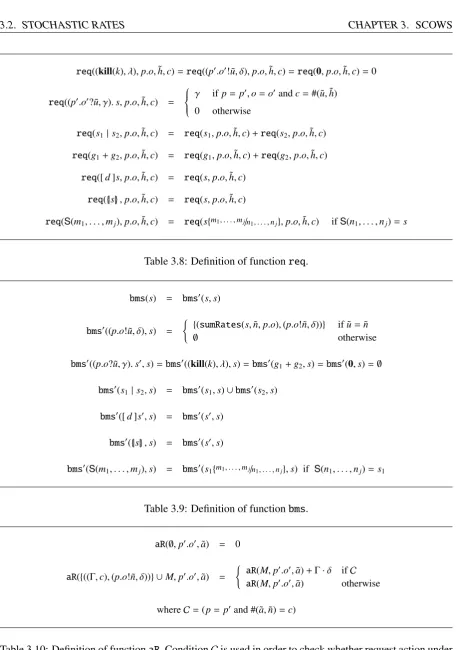
req(s,p.o,h˜,c) (cfr. Table 3.8) is built in a way similar toinv, and returns the sum of all rates of unguarded request actions in son endpoint pmatching with given tuple ˜hthrough ex-actlycsubstitutions. These actions are the ones competing with the selected request action (p.o?˜a, γ) for the communication at hand. Such sum allows us to compute the probability to choose that specific request action among all competitors: _req(_s_,γ_p_._o_,_h_˜_,_c₎. Notice that the fact that cis minimal (and thus that the selected request action is best-matching) comes directly from the existence of the communication transition itself.

bms(s) (cfr. Table 3.9) for each unguarded invoke action (p.o!ñ, δ) in s, returns a pair of the form ((Γ,c),(p.o!ñ, δ)), where (Γ,c) is the result ofsumRates(s,n˜,p.o) (see below), with Γ standing for the sum of all rates of the best-matching set for action p!ñ, and c representing the number of substitutions performed by the request actions belonging to such best-matching set. The resulting set of pairs B = bms(s) is used in aR(B,p.o,a˜) in order to compute the apparent rate of request action p?ãas described in Subsection 3.2.

sumRates(s,n˜,p.o) (cfr. Table 3.11) analyses service sand returns a pair of numbers (Γ,c), where Γis the sum of the rates of all request actions in the best-matching set for invoke action p.o!ñ and c is the number of substitutions through which these request actions match. Notice that, by the definition of best-matching set, c is the minimal number of substitutions with which any request action can match with p.o!ñ, and thus the sum of these rates is the apparent rate of a request action able to communicate only with p.o!ñ.

aR(B,p.o,a˜) (cfr. Table 3.10) computes the sum of the productΓ·δfor each pair of the form ((Γ,c),(p.o!ñ, δ)) in B and is used in order to compute the total apparent rate of request action p?ã defined as the average of the apparent rate of the request action (the sum of the rates of all request actions which could take its place in a communication) for each invoke action activating it. The average is weighted with the probabilities to choose each activating invoke action: e.g., the probability to choose (p.o!ñ, δ) is _aInv(_sδ_,_p_._o_,_a_˜₎, where sis the whole service.

(36)

req((kill(k), λ),p.o,h˜,c)=req((p0_._o0_!_˜u_{, δ}₎_,_p_._o_,_h_˜_,_c₎₌_req₍₀_,_p_._o_,_h_˜_,_c₎₌₀ req((p0_._o0_?_˜u_{, γ}₎_._s_,_p_._o_,_h_˜_,_c₎ ₌

      

γ ifp=p0_,_o₌_o0_and_c₌_{#( ˜}_u_,_h_˜₎

0 otherwise

req(s1|s2,p.o,h˜,c) = req(s1,p.o,h˜,c)+req(s2,p.o,h˜,c) req(g1+g2,p.o,h˜,c) = req(g1,p.o,h˜,c)+req(g2,p.o,h˜,c)

req([d]s,p.o,h˜,c) = req(s,p.o,h˜,c)

req({|s|},p.o,h˜,c) = req(s,p.o,h˜,c)

req(S(m1, . . . ,mj),p.o,h˜,c) = req(s{m1, . . . ,mj/n1, . . . ,nj},p.o,h˜,c) ifS(n1, . . . ,nj)=s

Table 3.8: Definition of functionreq.

bms(s) = bms0(s,s)

bms0((p.o!˜u, δ),s) =

(

{(sumRates(s,n˜,p.o),(p.o!˜n, δ))} if ˜u=n˜

∅ otherwise

bms0((p.o?˜u, γ).s0,s)=bms0((kill(k), λ),s)=bms0(g1+g2,s)=bms0(0,s)=∅ bms0(s1|s2,s) = bms0(s1,s)∪bms0(s2,s)

bms0([d]s0,s) = bms0(s0,s)

bms0({|s|},s) = bms0(s0,s)

bms0(S(m1, . . . ,mj),s) = bms0(s1{m1, . . . ,mj/n1, . . . ,nj},s) if S(n1, . . . ,nj)=s1

Table 3.9: Definition of functionbms.

aR(∅,p0_._o0_,_a_˜₎ ₌ ₀

aR({((Γ,c),(p.o!˜n, δ))} ∪M,p0.o0,a˜) =

(

aR(M,p0.o0,a˜)+ Γ·δ ifC aR(M,p0.o0,a˜) otherwise whereC=(p=p0and #(˜a,n˜)=c)

(37)

CHAPTER 3. SCOWS 3.2. STOCHASTIC RATES

sumRates((p0_.

o0

?˜u, γ).s,n˜,p.o)=

    

(γ,#( ˜u,n˜)) ifp=p0

ando=o0 (0,∞) otherwise

sumRates((p0_.

o0

!˜u, δ),n˜,p.o)=sumRates((kill(k), λ),n˜,p.o)=sumRates(0,n˜,p.o)=(0,∞)

sumRates([d]s,n˜,p.o)=sumRates(s,n˜,p.o)

sumRates({|s|},n˜,p.o)=sumRates(s,n˜,p.o)

sumRates(s1,n˜,p.o)=(γ1,c1) sumRates(s2,n˜,p.o)=(γ2,c2)

sumRates(s1|s2,n˜,p.o)=(γ3,c3)

(∗)

sumRates(g1,n˜,p.o)=(γ1,c1) sumRates(g2,n˜,p.o)=(γ2,c2)

sumRates(g1+g2,n˜,p.o)=(γ3,c3)

(∗)

(*) wherec3=min(c1,c2) andγ3=

          

γ1 ifc1<c2

γ2 ifc2<c1

γ1+γ2 ifc1=c2

sumRates(S(m1, . . . ,mj),n˜,p.o)=sumRates(s{m1, . . . ,mj/n1, . . . ,nj},n˜,p.o) if S(n1, . . . ,nj)=s

Table 3.11: Definition of functionsumRatesfor the calculation of the sum of rates in best-matching sets.

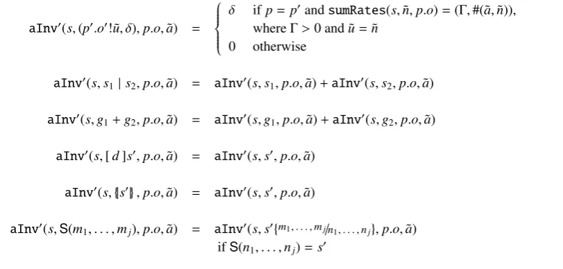
aInv(s,p.o,a˜) = aInv0₍_s_,_s_,_p_._o_,_a_˜₎

aInv0(s,(p0.o0?˜u, γ).s0,p.o,a˜)=aInv0(s,(kill(k), λ),p.o,a˜)=aInv0(s,0,p.o,a˜)=0

aInv0(s,(p0.o0!˜u, δ),p.o,a˜) =

          

δ ifp=p0_and_sumRates₍_s_,_n_˜_,_p_._o₎₌₍_Γ_,_#(˜_a_,_n_˜₎₎_,

whereΓ>0 and ˜u=n˜ 0 otherwise

aInv0₍_s_,_s

1|s2,p.o,a˜) = aInv0(s,s1,p.o,a˜)+aInv0(s,s2,p.o,a˜) aInv0(s,g1+g2,p.o,a˜) = aInv0(s,g1,p.o,a˜)+aInv0(s,g2,p.o,a˜)

aInv0₍_s_,_[_d_]_s0_,_p_._o_,_a_˜₎ ₌ _aInv0₍_s_,_s0_,_p_._o_,_a_˜₎ aInv0(s,{|s0|},p.o,a˜) = aInv0(s,s0,p.o,a˜)

aInv0(s,S(m1, . . . ,mj),p.o,a˜) = aInv0(s,s0{m1, . . . ,mj/n1, . . . ,nj},p.o,a˜) ifS(n1, . . . ,nj)=s0

(38)

Resuming, the rate of a stochastic execution step of a closed S service is computed as follows:

rates−−−−→ϑ(α)

ρ s

0 =

      

δ

inv(s,p.o)·

γ

req(s,p.o,h˜,#(˜a,˜h))·min

inv(s,p.o),aR(bms(s)_aInv(s_,_p,_.p_o._,o_a)_˜,a)˜ ifα=p.ob∅ca˜h˜

andρ=[γ, δ]

(39)

CHAPTER 3. SCOWS 3.3. STRUCTURAL CONGRUENCE IN SCOWS

3.3

Structural congruence in S



In this section, we will introduce a notion of structural congruence in S. This congruence is not to be applied directly in the operational semantics, as the introduction of a rule for the application of structural congruence goes against our objective to generate finitely branching transition systems. However, such a notion of congruence could become useful to identify services which, although grammatically different, originate the same behaviour.

Definition 3. The structural congruence relation of S is the least congruence relation≡ satisfying all laws in Table 3.13.

(prot₁) {|0|} ≡0 (prot₂) {|{|s|} |} ≡ {|s|}

(prot3) {|[d]s|} ≡[d]{|s|} (delim1) [d]0≡0

(delim2) [d1][d2]s≡[d2][d1]s (delim3) s1 |[d]s2≡[d](s1|s2)

ifd<fk(s2)

(par_assoc) s1|(s2|s3)≡(s1|s2)|s3 (parcomm) s1 |s2≡s2|s1

(par₀) s|0≡s (cho0) (p.o?˜u, γ).s+0≡(p.o?˜u, γ).s

(chocomm) g1+g2 ≡g2+g1 (choassoc) (g1+g2)+g3 ≡g1+(g2+g3)

Table 3.13: Structural congruence rules for S.

Notice that the rules are standard, with the only notable exception of a rule for idempotence of guarded sum, which does not apply in our case: as stated before (cfr. Sec. 3.1), we wish to distinguish between two services performing the same actions in a choice.

In [27] the authors show that the classical way of computing stochastic rates [36] for com-munication actions is in some cases imprecise, as it does not take into account the complete service in which the communication happens. This leads to the fact that two services differing only in the parenthesisation of their subcomponents, as could be (P | Q) | R and P | (Q | R) (which should be congruent by the associativity of parallel composition), give rise to transitions withdifferentstochastic rates: such a problem negates the congruence law for parallel associa-tivity. Nevertheless, our language still retains the associativity of parallel composition, as the communication rates are computed taking into account the whole service. This is due to the fact that COWS itself, through its polyadic matching rule, requires an analysis of the whole service before a transition is computed: the stochastic semantics follows this approach and the resulting rate computation method preserves the congruence relation.

(40)

Theorem 1. Given twoSservices P and Q such that P ≡ Q by the structural congruence law par_assoc, and such that P−−−−−ϑ1(α→)

ρ P

0

and Q−−−−−ϑ2(α→)

ρ Q

0

, we have that rate

P−−−−−ϑ1(α→)

ρ P

0 ₌

rate

Q−−−−−ϑ2_ρ(α→) Q0_.

Proof. As the congruence rule(assoc)states that (s1 | s2) | s3 ≡ s1 | (s2 | s3), we can suppose thatP≡ (s1 | s2)| s3andQ≡ s1 |(s2 |s3). Then, there are two cases based on the form ofα:

• α=†. Supposing that bothPandQhave chosen the same action (kill(k), λ), we have that

ρ= λand, by the computation of the rate for killing actions, the thesis.

• α = p.o b∅c a˜ h˜. In this case we have that ρ = [γ, δ] (where γ is the rate of the request action andδis the rate of the invoke action involved in the communication) and the rate is computed following equation (3.5):

rate

P−−−−−ϑ1(α→) [γ,δ] P

0₌ δ

inv(P,p.o)·

γ

req(P,p.o,h˜,#(˜a,h˜)) ·min

inv(P,p.o),aR_aInv(bms₍(_PP_,_p),_.p_o._,o_a_˜,₎a˜).

Now, for each of the functions involved in the computation of the rate we will show that the function preserves the associativity of parallel composition.

sumRates Given that

sumRates(s1,n˜,p.o)=(γ1,c1)

we have that

sumRates(s1 |s2,n˜,p.o)= (γ1,2,c1,2)

wherec1,2 =min(c1,c2) andγ1,2 =           

γ1 ifc1 <c2

γ2 ifc2 <c1

γ1+γ2 ifc1 =c2

sumRates((s1 |s2)|s3,n˜,p.o)= (γ,c)

wherec=min c1,2,c3 andγ=           

γ1,2 ifc1,2< c3

γ3 ifc3< c1,2

(41)

CHAPTER 3. SCOWS 3.3. STRUCTURAL CONGRUENCE IN SCOWS

while

sumRates(s2 |s3,n˜,p.o)= (γ2,3,c2,3)

wherec2,3 =min(c2,c3) andγ2,3 =           

γ2 ifc2 <c3

γ3 ifc3 <c2

γ2+γ3 ifc2 =c3

sumRates(s1 |(s2 |s3),n˜,p.o)=(γ0,c0)

wherec0 =min c1,c2,3 andγ0 =           

γ1 ifc1 < c2,3

γ2,3 ifc2,3 <c1

γ1+γ2,3 ifc1 = c2,3

Noticing that

c=min(min(c1,c2),c3)= min(c1,min(c2,c3))= c0

and that γ=                                 

γ1 ifc1 <c2andc1< c3

γ1+γ2 ifc1 =c2 <c3

γ1+γ3 ifc1 =c3 <c2

γ2+γ3 ifc2 =c3 <c1

γ1+γ2+γ3 ifc1 =c2 =c3

                                

=γ0

we can conclude that

sumRates((s1| s2)| s3,n˜,p.o)= sumRates(s1|(s2 |s3),n˜,p.o).

inv inv((s1|s2)|s3,p.o)=inv0((s1|s2)|s3,(s1|s2)|s3,p.o) =inv0

((s1|s2)|s3,s1|s2,p.o)+inv0((s1|s2)|s3,s3,p.o) =inv0

((s1|s2)|s3,s1,p.o)+inv0((s1|s2)|s3,s2,p.o)+inv0((s1|s2)|s3,s3,p.o)

Noticing thatinv’

returns a sum of integer numbers, and that in the base case where a non-zero value is returned it invokes function sumRates on the starting process P, we rely on the proof forsumRatesto complete the case forinv.

aInv This case is dealt the same way as the previous one.

req req((s1 |s2)|s3,p.o,h˜,c)=req(s1 | s2,p.o,h˜,c)+req(s3,p.o,h˜,c) =req(s1,p.o,h˜,c)+req(s2,p.o,h˜,c)+req(s3,p.o,h˜,c)

=req(s1,p.o,h˜,c)+req(s2| s3,p.o,h˜,c)=req(s1 |(s2 |s3),p.o,h˜,c)

bms bms((s1 |s2)|s3)=bms0((s1 |s2)| s3,(s1| s2)| s3) =bms0(s1 |s2,(s1 | s2)| s3)∪bms0(s3,(s1 |s2)|s3)

=bms0(s1,(s1 |s2)| s3)∪bms0(s2,(s1 |s2)|s3)∪bms0(s3,(s1| s2)| s3)

(42)

aR As can be derived from the definition of aR, no reference to services is made, so the function does not need to be taken into account.

We can then conclude that

rate

P−−−−−ϑ1(α→)

[γ,δ] P 0₌

rate

Q−−−−−ϑ2(α→)

[γ,δ] Q 0_.

3.4

Final considerations on S



(43)

Chapter 4

A tool for model checking S



In the conclusion of Chapter 3 we highlighted the fact that generating a CTMC from a S model can be a computationally costly task, as it would require the generation of the complete transition system of the model. The main problem that the generation of a complete transition system for a non-trivial Smodel would cause is the notorious state space explosion prob-lem. This kind of problem is most evident when a model comprises a number of loosely coupled components, as is often the case when dealing with distributed systems. The problem comes from the observation that the transition graph of a system composed ofxprocesses in parallel, each of which withystates, can have (in the case that no communication happens among the processes) up toyx states. A compositional generation of the transition system (and thus, of the underlying CTMC) would allow to avoid the problem of state space explosion, thanks to the fact that parallel components are considered in isolation and then merged with less-than-exponential execution time. Unfortunately, this type of approach can not be applied in the case of S. This is because of the name-passing matching paradigm adopted by the language, which requires to know an entire model to calculate a single communication action, preventing de facto any compositional approach to the transition system generation. In languages with-out the name-passing feature such as PEPA [22], the compositional approach can be applied and is in fact feasible: an approach of this kind is used for the generation of a CTMC from a PEPA model in PRISM [24], which is based on MTBDD (multi-terminal binary decision dia-grams, [15, 20]) representations. Another example of application of the same principle is the

CASPAtool [29], which generates a MTBDD representation fromYAMPA, a stochastic process

calculus based on TIPP [21].

In this chapter we will present our proposed solution to the problem of model checking S models avoiding the generation of the full transition system: S amc. This tool distinguishes itself from the other stochastic model checking tools because it makes use of a simulation-based approach for the verification of properties without generating the full transi-tion system of a model. This allows us to avoid the problem of state space explosion, while still maintaining acceptable computation time and approximation values.

(44)

is that an integration with other tools from the SENSORIA project [2] is planned, and having a common implementation language would greatly simplify the integration process.

4.1

Overview on the approach

In order not to generate a complete transition system, and thus avoid the state space explosion problem, we base our model checking approach on the direct simulation of Smodels. This means that we generate a number of simulation traces by applying the operational semantics presented in Chapter 3 directly to Sservices, and then perform the computations necessary to check the desired formula against these traces. As a single execution trace of a stochastic model is by definition a random walk on the transition system of the model, we have to resort to statistical reasoning in order to estimate the size of the error we make in evaluating the requested property through a finite number of random walks. The theories behind the reasoning on which the approach used by the S amc tool is based are the one adopted in the Ymer tool [18] (mainly consisting of Wald’s sequential probability ratio test[39]) and the one adopted in the APMC tool [19]. S amc differentiates from both because it is based on S models, while the others are based on CTMCs.

The CSL [5] formulas on which we will concentrate our efforts can be expressed in one of the following forms:

P./θ[Ψ1U[t0,t1] Ψ2], where ./ ∈ {<,6, >,>}andθ∈[0,1] (4.1) or

P₌_?[Ψ1 U[t0,t1] Ψ2_] _(4.2)

and can be read respectively as “Is there a probability p ./ θ that state formula Ψ1 will hold until, inside the time interval [t0t1], state formulaΨ2 holds?” and “What is the probability that state formulaΨ1 will hold until, inside the time interval [t0t1], state formulaΨ2holds?”. State formulae Ψ1 andΨ2 are to be intended as state labels or as formulae of type 3/4 themselves. As we will see, the approach used in Ymer will be employed to decide the truth value of CSL formulas of type (4.1), while the method applied in APMC will be used in the estimation of formulas of type (4.2).

In the following subsections we will give an explanation of the theory and the observations on which the S amc tool is based.

4.2

Statistical hypothesis testing

The approach employed in the Ymer tool is based on a theory of statistical hypothesis testing, which we will resume here.

First of all, notice that the property P_>θ[ΦU[t0,t1] Ψ_{] is equivalent to} _{¬ P}

(45)

CHAPTER 4. SCOWSAMC 4.2. STATISTICAL HYPOTHESIS TESTING

For this reason, we will explain the statistical hypothesis testing theory taking into account only the formulaP_>θ[ΦU[t0,t1] Ψ_{] without losing generality w.r.t. the other forms described in (4.1).} The formula, which corresponds to the assertion “the probability that formula ΦU[t0,t1]Ψ _is true if tested on a random walk starting from the initial state of the given S model is at leastθ”, will be represented from now on by the hypothesisH =“p_> θ”.

The hypothesis testing problem takes into account the probability to have an error in the observation of an event, and thus to find the hypothesis to be false while it is actually true (false negative), or to state that the property is true when it is false (false positive). We will choose limits to the occurrence of the two types of error, and in particular we set the probability to have a false negative (i.e., to reject Hwhen it is true) to be at most α, and the probability to have a false positive (i.e., to acceptHwhen it is false) to be at mostβ, withα+β₆1.

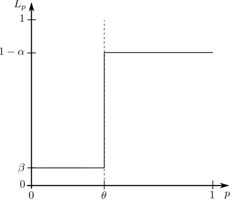
In Figure 4.1 we show the graph of the ideal testing environment, where the probability of false negative is exactlyαand the probability of false positive is exactlyβ. The graph presents a

Figure 4.1: The probabilityLpto accept hypothesisH=“p>θ” as a function ofp. Ideal case.

plot of the probability to accept hypothesisHas a function of the probability p. As can be seen,

whenp < θ(and thus, the hypothesis “p_> θ” is false), the probability to accept the hypothesis

equalsβ(as it is the probability of a false positive), while whenp> θthis probability becomes 1−α (asαis the probability to have a false negative). In the point where p = θ, we request the probability to acceptH to be both equal to 1−αand toβ. Thus, it must be thatβ = 1−α, preventing us to choose the values ofαandβindependently.

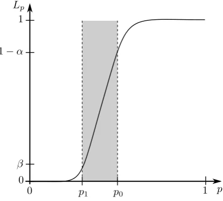
In order to be able to set the error probabilities αand β independently from each other, a relaxation of the threshold becomes necessary: in particular, an indifference region is intro-duced. This region corresponds to all values of pbetween two thresholds p1and p0 for which

θ−δ = p1 < θ < p0 = θ+ δ holds. The value δ determines the amplitude of the region in

(46)

against its negate to testingH0 =“p> p0” against H1 = “p6 p1”. Maintaining the conditions onαandβ, we present in Figure 4.2 a realistic hypothesis testing case. In this case, the original

Figure 4.2: The probabilityLpto accept hypothesisH0=“p> p0” as a function ofp. Real case.

hypothesis H = “p _> θ” is accepted with probability at least 1−αif p _> θ+δ (because hy-pothesisH0 is accepted), and is rejected with probability at mostβif p6 θ−δ(hypothesisH1 is accepted). If p ∈(p1,p0), both hypothesesH0andH1 are false, as in the indifference region it is indifferent which of the two hypotheses is accepted. In Figure 4.2 this region is marked by a gray area. Notice that decreasing the value ofδ, and thus narrowing the indifference region, it is possible to get closer to the ideal hypothesis testing situation of Figure 4.1.

In the next section we will present a statistical method which allows to test the described hypothesisHwith the chosen probabilities of errorαandβ.

4.3

The sequential probability ratio test

The sequential probability ratio test has been introduced by Wald in [39], and is a statistical test where the number of observations is not determineda priori. Instead, the test allows to decide whether the given hypothesis is true or false when the error evaluation crosses a predetermined threshold. If a decision cannot be made, a new observation is made.

In our case, remembering that we have defined an indifference region between probabilities p1 =θ−δand p0= θ+δ, the hypothesis to be tested at each iteration isH0 =“p> p0”, and its converse isH1 =“p6 p1”. After having perf