The Thirty-Third AAAI Conference on Artificial Intelligence (AAAI-19)
SCNN: A General Distribution Based Statistical
Convolutional Neural Network with Application to Video Object Detection
Tianchen Wang,
1Jinjun Xiong,
2Xiaowei Xu,
3Yiyu Shi
41,3,4Department of Computer Science and Engineering, University of Notre Dame 2IBM Thomas J. Watson Research Center
{1twang9,3xxu8,4yshi4}@nd.edu,2[email protected]
Abstract
Various convolutional neural networks (CNNs) were devel-oped recently that achieved accuracy comparable with that of human beings in computer vision tasks such as image recog-nition, object detection and tracking, etc. Most of these net-works, however, process one single frame of image at a time, and may not fully utilize the temporal and contextual correla-tion typically present in multiple channels of the same image or adjacent frames from a video, thus limiting the achievable throughput. This limitation stems from the fact that existing CNNs operate on deterministic numbers. In this paper, we pro-pose a novel statistical convolutional neural network (SCNN), which extends existing CNN architectures but operates directly on correlated distributions rather than deterministic numbers. By introducing a parameterized canonical model to model correlated data and defining corresponding operations as re-quired for CNN training and inference, we show that SCNN can process multiple frames of correlated images effectively, hence achieving significant speedup over existing CNN mod-els. We use a CNN based video object detection as an example to illustrate the usefulness of the proposed SCNN as a general network model. Experimental results show that even a non-optimized implementation of SCNN can still achieve 178% speedup over existing CNNs with slight accuracy degradation.
Introduction
With strong feature extraction capabilities from deep convo-lutional neural networks (CNNs) and many optimized imple-mentations (Xu et al. 2017) of the associated deep learning frameworks, the performance of various computer vision tasks has been drastically improved. For example in image recognition and object detection, deep CNN architectures as ResNet (He et al. 2016), DenseNet (Huang et al. 2017) and frameworks as YOLO (Redmon and Farhadi 2017), faster R-CNN (Ren et al. 2015) all outperform then state-of-the-art by an impressive margin at the time of their publication.
However, a mainstay for any CNN based framework is that it operates on deterministic weights and inputs (Xu et al. 2018a; 2018b). These frameworks process one image at a time during both training and inference. This is obviously not ideal as it largely ignores both temporal and contextual corre-lation existing among channels and adjacent frames. To break
Copyright c2019, Association for the Advancement of Artificial Intelligence (www.aaai.org). All rights reserved.
this mainstay, in this paper we propose to explicitly model such correlation by extracting parameterized canonical distri-butions from correlated inputs (such as adjacent frames in a video), and design a statistical convolutional neural network (SCNN) to propagate these correlated distributions directly. Our SCNN can be easily integrated into existing CNN archi-tectures by replacing their deterministic operations with our statistical counterparts operating on parameterized canonical distributions. Then with little modification to the existing gradient descent based scheme, our SCNN can be trained using the same forward and back propagation procedures.
More specifically, we first build a linear parameterized canonical form via independent component analysis (ICA) to represent the statistical distribution of each input com-ponent to capture its temporal and contextual correlation. We then define all the required CNN operations (such as convolution, ReLU, batch normalization etc.) in terms of the parameterized canonical form, including their various partial gradients for backward propagation, thus enabling us to integrate SCNN with any existing CNN implemen-tation frameworks easily. To show the effectiveness of the proposed SCNN, we further apply it to video object detec-tion task and propose a new objective funcdetec-tion that improves SCNN based training. Even though many great successes have been achieved in objection detection for static images (Ren et al. 2015; Redmon and Farhadi 2017; Lin et al. 2018; Liu et al. 2016), the performance of video object detection still has a large room for improvement, especially for its real-time throughput. Since its introduction in ImageNet competi-tion, multiple solutions have been proposed (Kang et al. 2017; Han et al. 2016), most of which solve the problem by extend-ing static image object detection methods to consider adjacent frames for temporal information. Their efficiency is, how-ever, not satisfactory for online detection, and for training, it would take several days to generate video tubelets (Kang et al. 2017). A recent research (Zhu et al. 2017) proposed a flow-guided feature aggregation where it considers adjacent frames at feature level rather than at the box level, but it requires repeated sampling and complex modeling. It is still desirable to have a more direct and effective way of modeling correlated adjacent frames.
ar-chitectures and operates directly on distributions rather than deterministic numbers, 2) We use a parameterized canon-ical model to capture correlated input data for CNN and reformulate popular CNN layers to adapt their forward and backward computation for parameterized canonical models. 3) We adopt video object detection as an examplar applica-tion and introduce a new objective funcapplica-tion for better training of SCNN. 4) We conduct experiments on an industrial UAV object detection dataset and show that SCNN backbone can achieve up to178%speedup over conventional counterpart with slight accuracy degradation.
Review of ICA
ICA is a well-known technique in signal processing to sep-arate a multivariate signal into a set of additive random subcomponents that are statistically independent from each other. The random subcomponents are typically modeled as non-Gaussian distributions. In some cases, a priori knowl-edge of the probability distributions of these random sub-components can be also incorporated into ICA. The ran-dom subcomponents are also called the basis of the corre-sponding multivariate signal. We denote an n-dimensional multivariate signal as a random vectorD=(D1,D2,...,Dn)T. The random subcomponents are denoted as a random vector
X=(X1,X2,...,Xm)T. For a given set ofN samples (real-izations) of the multivariate signal’s random vectorD, each componentDiof theNsamples can be treated as being gen-erated by a sum of some realization of themindependent random subcomponents, which is given by
Di=ai,1X1+ai,2X2+···+ai,kXk+···+ai,mXm, k∈{1,m} (1) whereai,kis the mixing weight of the corresponding random subcomponentXk. We can put them compactly in a matrix form as follows
D=AX (2)
whereAis the mixing matrix. The goal of ICA is to estimate both the mixing matrixAand the corresponding realization of the random subcomponentX(i.e.,X=W D). The realization of the basisX can be obtained either by invertingAdirectly (i.e.,W=A−1) or through the pseudo inverse ofA.
The ICA has also been extended to consider the case where a zero-mean uncorrelated Gaussian noiseRiis added. With-out loss of generality, we can normalize all basis (random subcomponents) to have a zero mean and standard deviation of 1. In other words, we have
Di=ai,0+ai,1X1+ai,2X2+···+ai,mXm+ai,rRi (3) whereai,0is the mean value forDi, andai,ris the weighting of the modeled uncorrelated Gaussian noise term.
Statistical Convolutional Neural Network
Correlated Inputs Modeling
Many existing applications with CNN models have inputs that exhibit strong temporal and contextual (spatial) corre-lations, such as multiple adjacent frames in a video stream. Therefore, we can model these inputs as a multivariate signal. For a given set ofN samples (realizations) of the inputs,
-3.0 -2.0 -1.0 0.0 1.0 2.0 3.0
Basis Extraction Error(%) 0
20 40 60 80 100 120 140 160
Probability Density
0.250 0.375 0.500 0.625 0.750 0.875
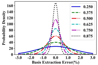
Figure 1: ICA modeling error (%) with differentm/N.
such as multiple correlated frames of a video snippet, we can represent each component of the inputs via ICA as a linear additive model of a set ofmindependent random subcompo-nents as shown in Equation (3). In the rest of the paper, we defineN as extraction span andmas the basis dimension. Moreover, because the random subcomponentsX1,...,Xm are shared among all input components, we can use the above model to compactly capture both the temporal and contextual correlations. We call such a model as a linear parameterized canonical model, and the weights such asai,kas parameters.
To demonstrate the accuracy of ICA to model correlated frames in a video, we extract the distributions from a few small video snippets in our experiment dataset (DAC-Contest 2018) and depict the error distribution between the original data and the mixing result in Figure 1. From the figure we can see that increasing the ratio ofm/Nin general reduces the error, and the error is mostly bounded by3%.
In the context of CNN, this type of modeling of correlated inputs raises a number of interesting questions. (1) For a given trained CNN network with model parameters, how do we carry out the inference for such a parameterized canonical model? (2) How to train such a CNN network with each input being represented as a parameterized canonical form? We will provide answers to address the above two questions in the rest of the paper.
Correlated inputs
T Sets
Outputs Neural network
processing with distributions
Canonical model extraction ICA
… … … …
…
Basis distributions
Each pixel is a distribution
Evaluation
Wi,jl …
…
Statistical operation
Basis values of each images set
1st image:{a
1,0, a1,1, a1,2,…} 2ed image:{a
2,0, a2,1, a2,2,…}
…
Distributions
X:
Coefficient vectors
Data:
Coefficient vectors for distributions
Weight:
Deterministic numbers
Wi,jl
Targets
1 Set of N images
T Sets 1 Set of N images
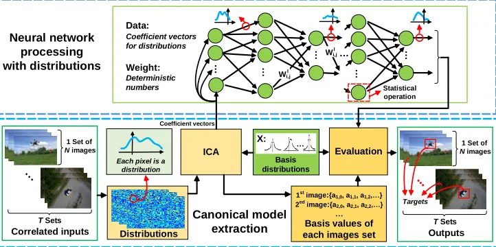
Figure 2: Overall structure of SCNN (illustrating an object detection task in a video).
Forward Propagation in SCNN
In a typical CNN network, there are a number of commonly used layers, such as fully connected layer (FC), convolutional layer (CN), ReLU layer, max-pooling layer, batch normaliza-tion layer. We will provide the corresponding implementanormaliza-tion details in SCNN for these commonly used layers in the fol-lowing. Again we would like to emphasize that the discussion here does not restrict to any particular CNN architecture. In our experiments we will demonstrate our implementation on various CNN architectures.
Before we delve into the details of each layer imple-mentation, we note that there are two core operations for these layers: (1) a weighted sumof a set of input num-bers (which is used frequently for both FC and CN lay-ers), and (2) a max of a set of input numbers (which is frequently used for both ReLU and max-pooling layers). In SCNN, the input numbers to the above two operations are no longer deterministic numbers, but parameterized sta-tistical distributions. We discuss how we provide solutions to these two core operations first. Please note that, some of the discussion related to the sum and max operations has been covered in prior literature in the area of statistical timing analysis (Xiong, Zolotov, and Visweswariah 2008; Cheng, Xiong, and He 2009; Visweswariah et al. 2006; Singh and Sapatnekar 2006). We obtain a lot of inspiration from their work. We only repeat essential points in this pa-per for completeness, but refer interested readers to those references for greater details and proofs.
Sum operation For two inputsDiandDj, their sum can be represented as
Dsum=Di+Dj
=(ai,0+aj,0)+(ai,1+aj,1)X1+(ai,2+aj,2)X2+...
+(ai,m+aj,m)Xm+ai,rRi+aj,rRj.
(4) As we can see, thesumoperation as defined above will give us back a similar parameterized canonical form. This
is important as it allows us to carry out similar operations repeatedly across layers. Because of this, for multiple inputs, similar sum operations can be applied easily. Most interest-ingly, the computation involves only those parameters, but not random subcomponents.
Max operation Themaxoperation is a bit more involved. We start with the most common scenario where the distribu-tion of random subcomponentsX1,...,Xmare modeled as a Gaussian distribution. In this case, for two inputsDiandDj, their max can be represented as
Dmax=max(Di,Dj)=amax,0+
m X
k=1
amax,kXk+amax,rRmax (5) whereamax,0andamax,rare obtained by matching the first and2ndmoments of the above equation on both sides;a
max,k are obtained via the tightness probabilities as introduced in (Visweswariah et al. 2006) to represent the probability that one distribution is larger than (or dominates) the other given by
ti=
Z ∞
−∞
1 σDi
φ(x−ai,0 σDi
)Φ( (x−aj,0
σDj )−ρ( x−ai,0
σDi ) p
1−ρ2 )dx=Φ(β)
(6) whereθ,β,φandΦare defined as
θ=qσ2
Di+σ
2
Dj−2σDiσDj, β=(
ai,0−aj,0
θ ),
φ(x)=√1
2πexp(− x2
2 ), Φ(y)=
Z y
−∞
φ(x)dx.
(7)
Therefore, the meanamax,0and varianceσD2maxofDmaxcan
be expressed analytically as
amax,0=ai,0Φ(β)+aj,0Φ(−β)+θφ(β),
σ2Dmax=(σ2Di+a2i,0)Φ(β)+(σ2Dj+a2j,0)Φ(−β) +(ai,0+aj,0)θφ(β)−a2max,0.
And the corresponding canonical form ofDmaxis
Dmax=amax,0+
m X
k=1
amax,kXk+amax,rRmax where amax,k=Φ(β)ai,k+Φ(−β)aj,k, k={1,m},
amax,r=(σD2max−
m X
k=1
a2max,k)1/2.
(9)
It is noted thatσ2
Dmax−
Pm k=1a
2
max,k is proved to be always non-negative by (Sinha, Shenoy, and Zhou 2005). For sim-plicity, we useΦand φto representΦ(β)and φ(β), and
sumandmaxto represent the statistical operations between distributions, and the notations will be used wherever there is no ambiguity.
Same as thesumoperation, themaxoperation as defined above will give us back a similar parameterized canonical form. This is important as it allows us to carry out similar max operations repeatedly across layers. Because of this, for multiple inputs, we can repeatedly apply the two input max operations and obtain the final multi-input max result, i.e.,
max(D1,D2,...,Dp)=max(D1,max(D2,max(D3,....)))).
(10) In the same spirit, more sophisticated approaches to handle themaxoperation of multiple inputs and non-Gaussian distri-butions have been discussed in references such as (Xiong et al. 2006; Mogal et al. 2007). In the interests of space, we’ll not repeat it here.
FC & CN layers Key to the two layers’ operation is the computation of a weightedsum. When the inputs are parame-terized canonical form, we can decompose the weighted sum in two logic steps: (1) for each input, we scale the input by the weight and obtain a similar canonical form; and (2) for the remaining sum operation, it is carried out same as the sum of a set of canonical forms.
For FC, given an input withpdistributionsDl
i(i∈{1,p}) at layerl, the forward operation computes the jth output distributionsDlj+1(j∈{1,q})with weightwas:
Dlj+1=alj,+10+
m
X
k=1
alj,k+1Xk+alj,r+1R= p
X
i=1 wi,jDli
=
p
X
i=1
wi,jali,0+ p
X
i=1 m
X
k=1
wi,jali,kXk+
v u u t
p
X
i=1
(wi,jali,r)2R.
(11)
For CN, an input distribution tensor would be given asDl∈ Rm+2,h,w(h×wdistributions at layerl) and a convolution filterW∈Rx0,y0 (x0,y0denote the convolution kernel mask size) for the next layer, we have the forward propagation for
SCNN CN at positionx,yexpressed as
Dx,yl+1=a l+1
x,y,0+
m X
k=1
ax,y,il+1 Xi+ax,y,rl+1 R=Dlx,y∗Wx,y
=X
x0
X
y0
Wx0,y0alx−x0,y−y0,0
+X
x0
X
y0
m X
k=1
Wx0,y0alx−x0,y−y0,kXk
+
s X
x0
X
y0
(Wx0,y0al
x−x0,y−y0,r)2R,
(12)
where∗denotes the convolution operation.
ReLU and max-pooling layers Since the key operation in both ReLU and max-pooling layers is themaxoperation, we can easily extend themaxoperation as discussed above to handle the canonical inputs. In the case of ReLU, the reference point is not necessary to be zero, and it can be defined as a distribution. But in our current implementation, we still choose a constant reference for ReLU.
In max-pooling layer, new distributions are generated from the previous layer distributions under sliding masks withmax
operation. Given an input distribution tensorDl∈Rm+2,h,w, and amaxpooling filterK∈Rhf,wf, the problem is to obtain
an output distribution tensorDl+1ofmaxdistribution from partitioned subtensors. Therefore the forward propagation with stridesand without padding can be expressed as
Dlx,y+1= max
(x,y)∈[s×x,s×x+hf]×[s×y,s×y+wf]
Dlx,y. (13)
In traditional max-pooling layer, the locations of maximum values at the current layer under kernel masks are stored for back propagation. During SCNN max-pooling implementa-tion, we store the tightness probabilities between the corre-sponding distributions during forward propagation, which indicate the contributions of the distributions at the current layer to the ones at the next layer.
Batch normalization layer In SCNN, we do not follow the traditional batch normalization layer (Ioffe and Szegedy 2015) definition. Instead, we define the operation as follows in consideration of the canonical inputs: given an input dis-tributionDl
iwith basis sensitivityai,kand varianceσD2l i
, the normalization output distributionDli+1is expressed as
Dil+1=ali,+10+
m X
k=1
ali,k+1Xk+alr+1Ri
=ali,0+
m X
k=1
(γa
l i,k−
1
n Pm
j=1a
l i,j q
σ2
Dl i
+
+β)+alrRi, (14)
Inference at the output layer After we carry out the pa-rameterized forms through the various layers in the CNN network as discussed above, we arrive at the end of the net-work where we need to decide the output. Here we resort to a simple approach, i.e., we convert the canonical forms to their corresponding scalar values by plugging the estimated real-izations of random subcomponentsX=W D. With that, we obtain the output layer with scalar values, hence conventional inference at the last output layer can be carried out.
Back Propagation in SCNN
The back propagation is key to the training of the SCNN by computing various gradients of the cost function with respect to network parameters, which in term depends on computing the partial derivatives of various operation outputs with respect to their inputs.
Partial derivative for sum Given two distributionsDi,Dj along with two weightswi,wj,and the sumDsum=wiDi+
wjDj, the partial derivative ofDsumw.r.t. the sensitivities in
Diis expressed as
∂Dsum
∂ai,k
=wi,
∂Dsum
∂ai,r
= wi asum,r
(15)
wherek∈{0,m}. Then with the help of gradient ofsum oper-ation, the derivatives of FC and CN in SCNN are obtained accordingly. Given the gradient ofDjl+1at layerl+1asδjl+1
(j∈{1,q}), the gradients of each sensitivities in distribution
Dl
i(i∈{1,p}) at layerlare shown as
δi,kl =
q X
j=1
δjl+1∂D
l+1 j ∂al i,k = q X j=1
δjl+1wi,j, k∈{0,m},
δli,r=
q X
j=1
δjl+1∂D
l+1 j ∂al i,r = q X j=1
δjl+1wi,j aln,k+1.
(16)
The partial derivatives of total costLw.r.t. corresponding weightwi,jin FC goes to
∂L ∂wi,j
=δlj+1∂D
l+1
j
∂wi,j
=δjl+1(
m X
k=0
ali,k+a
l i,r
alj,r+1). (17)
The derivative of SCNN CN layer follows the same path. Given the gradient ofDl+1 w.r.t. total costLasδl+1, the
gradients of each sensitivities in distributionDlx,yat location
x,yasδx,yl are shown as
δx,y,kl = ∂L ∂al
x,y,k
=δlx,y,k+1 ∗W−x,−yl+1 , k∈{0,m},
δx,y,rl =
∂L ∂al
x,y,r
=δ
l+1
x,y,ralx,y,r
alx,y,r+1
∗(W−x,−yl+1 )2.
(18)
The gradient of convolution weight is derived as
∂L
∂Wx,yl+1
=
m X
k=0
δx,y,kl+1 ∗al−x,−y,k+δ
l+1
x,y,rWx,yl+1
alx,y,r+1
∗(al−x,−y,r)2.
(19)
Partial derivative for max The derivative ofmaxin distri-butions is mainly involved in the back propagation of SCNN ReLU and Max-pooling layer. Given two distributionsDi andDj withDmax=max(Di,Dj), the gradient of mean and variance ofDmaxwith respect toDi is derived by (Xiong, Zolotov, and Visweswariah 2008). We follow the similar rou-tine and derive the gradients of each sensitivities ofDmax with respect to the ones ofDi.
ReLU and max-pooling layers For ReLU, the derivation ofmaxis applied directly since themaxis used independently among distributions. For max-pooling, since the result is ob-tained by repeatedly applying the two input max operations, the gradients of the input distributions are obtained by itera-tively applying the derivation ofmaxwith the stored tightness probabilities.
Partial derivative for batch normalization Since the re-formulated batch normalization layer does not have distribu-tion operadistribu-tions involved, the derivative follows the tradidistribu-tional approach. Given the gradient of lossL, the gradients of sen-sitivities in distributionDl
iare ∂L ∂al i,k = m ∂L
∂ˆali,k+1− Pm
j=1
∂L ∂ˆalj,k+1−ˆa
l+1
i,k Pm
j=1
∂L ∂ˆalj,k+1ˆa
l+1
j,k
mqσ2
Dl i + , ∂L ∂γ= m X k=1 ∂L
∂ali,k+1ˆa
l+1 i,k , ∂L ∂β= m X k=1 ∂L
∂ali,k+1
(20) whereˆalj,k+1=(aj,kl+1−β)/γandk∈{1,m}.
Training, Inference, and Complexity Analysis
With back propagation as discussed above, the training can be easily carried out as follows. The distributions are first extracted by ICA with a predefined extraction span. The extracted distributions then propagate through the constructed SCNN layers. Before entering the evaluation module, the propagated distributions are mixed to form a temporal feature map. When the loss is obtained after evaluation with the proposed objective function, the error is propagated backward through the derived route. The gradients of the canonical form distributions are calculated to act as the gradient outputs of the corresponding layers. Then the weights with deterministic numbers are updated based on the obtained gradient outputs and the predefined learning rate.
The speedup of SCNN mainly comes from the fact that
N input images are modeled by a single parameterized canonical model of the same size. On the other hand, the computation complexity at each layer, including max,
sum and assigning weights in forward propagation is in-creased by O(m). In addition, SCNN requires the extrac-tion of the parameterized canonical model by ICA at the input, which incurs additional complexity overhead. For-tunately, with the fast ICA implementations available on GPUs, the execution time is negligible compared with the SCNN inference time (Ramalho, Tomas, and Sousa 2010; Kumara et al. 2016). As such, networks with SCNN back-bone can achieve an inference speedup of approximately
Extension to Nonlinear Canonical Form
Note that so far we have only discussed the linear parame-terized canonical form obtained from ICA and its associated extension to various CNN layers. It is also possible to obtain other nonlinear parameterized canonical form as suggested by (Singh and Sapatnekar 2006; Cheng, Xiong, and He 2009) in a different context. We believe such an extension can be adopted for the proposed SCNN as well. For simplicity, we will not discuss it further in this paper but defer it as our future work.
Video Object Detection: an Application
We believe SCNN can be a general and powerful backbone to any CNN networks and it processes parameterized statistical distributions rather than a deterministic values. Many CNN-based applications would benefit from such a representation. As a proof of point, we apply SCNN to the video object de-tection task to show its usefulness. Please note that, our initial implementation of SCNN (i.e., the statistical version of FC, CN, ReLU, Max-pooling and Batch normalization etc.) is far from perfection compared to those matured implementations in existing frameworks such as TensorFlow, Caffe, PyTorch. Because of that, our current implementation of SCNN to solve the video object detection is not yet optimized. Hence it is not our intention in this paper to compete in either train-ing performance or inference quality with the state-of-the-art video object detection techniques such as Faster R-CNN, YOLOv2/v3 etc (Ren et al. 2015; Redmon and Farhadi 2017; 2018), although we have shown the theoretic performance advantage. Instead, we want to use our implementation to show the great potential of SCNN for solving important com-puter vision problems and where it can potentially shine. In solving the video object detection problem, we proposed a few modifications to the commonly used object detection techniques in the context of SCNN.
We first replace a few commonly used backbone CNN networks for object detection with the proposed SCNN, in-cluding VGG11, VGG16, ResNet18 and ResNet34. We then add a simple evaluation module consisting of conv-relu-conv-relu-conv layers without padding. Because SCNN can ef-fectively process multiple frames at the same time, a few changes need to be made when designing the detection layer and the objective function.
For simplicity, we start with the case where there is only a single target object in videos and design a simplified de-tection layer based on YOLOv2 framework(Redmon and Farhadi 2017). In the detection layer of YOLOv2, predefined anchor boxes along with their confidence are predicted at each sub grid cell (13×13total) to detect objects. Such an approach is, however, not directly applicable to process video snippets with a continuously moving object captured by a sin-gle canonical model. Therefore, we propose a new detection layer with five predefined anchors (ai,w,ai,hfori∈{0,4}) at the center of the map (effectively treating the map as a single big cell). The network predicts coordinates for the box (tx,
ty,tw,th) along with its confidence. These predictions in
turn define the predicted bounding box as follows:
bx=σ(tx), bw=
ai,w
β log(1+exp(βtw)),
by=σ(ty), bh=
ai,h
β log(1+exp(βth))
(21)
whereσdenotes the sigmoid function andβ is for the for-mulation of Softplus. Note that we use Softplus function to configure the widthbwand heightbhrather than direct expo-nential as was used in YOLOv2. This modication brings a more stable and smooth transformation on anchor size and fit well with our one big cell setting.
Since SCNN simultaneously handles multiple frames, the detection objective function should not only consider the pre-cision on a single frames, but also account for the continuity of objects among adjacent frames. As such, we propose a new objective function for SCNN, which is a combination of co-ordinatesl2loss (Lcoord), confidence loss (Lconf), polynomial
fitting loss (Lfit), and IOU loss (LIOU).
The IOU loss is first introduced in UnitBox(Yu et al. 2016), which increases the accuracy by regressing the prediction box as a whole unit. However, the curve of natural logarithm used in Unitbox has a steep slope, which is weak when the IOU gets high and needs fine-tuning. Moreover, if we only use the IOU loss in the objective function, it would remain constant when the prediction box is out of the target area. This will not be helpful to improve the convergence of training. Intuitively, we would prefer an IOU loss that can compensate the coordinates loss to further increase the IOU. Therefore, in this work, we propose to use a negative log sigmoid function of IOU. Moreover, different from YOLOv2 where IOU is included in the confidence score, we use confidence lossLconf to detect whether there is an object or not.
To further improve the accuracy, we observe that within the frames in the extraction span, the trajectories of object bounding box coordinates can be approximated by a polyno-mial curve. After predicting coordinates with Equation 21, we adopt the least-square polynomial fitting to obtain the corrected coordinates along with the fitting lossLfit. The loss is then appended to the objective function as a penalty term. In summary, given an initial bounding box prediction
z=(bx,by,bw,bh,Cz), after fitting correctionzˆ and its cor-responding ground truthz˜, the IOU betweenzand˜zmarked asXz,˜z, the objective functionL(z,z˜)is expressed as:
L(z,z˜)=λcoordLcoord+λfitLfit+λconfLconf+λIOULIOU
=λcoord X
i∈{x,y,w,h}
(zi−z˜i)2+λfit X
i∈{x,y,w,h}
(zi−zˆi)2
+λconf( X
1obj(Cz−C
˜
z)2+ X
1noobj(Cz−C
˜
z)2)
−λIOUln(
1
1+exp(−αX(z,z˜)))
(22)
Models VGG11 VGG16 ResNet18 ResNet34
m - 8 10 12 14 - 8 10 12 14 - 8 10 12 14 - 8 10 12 14 mAP 62.2 56.5 58.1 58.3 58.7 61.9 57.1 57.2 57.7 58.3 65.1 57.4 58.7 60.0 61.9 64 56.7 59.2 60.5 62.2
FPS 101 181 150 130 116 65 116 98 84 72 247 363 340 304 276 161 246 225 210 188
Table 1: Accuracy/speed comparison between networkswithSCNN backbone (configured with various basis dimensionmand fixed extraction spanN=16) andwithoutSCNN backbone (marked with−in Rowm).
Category boat building car drone horseride paraglider person riding truck wakeboard whale w/o SCNN 90.0 91.3 60.7 50.1 40.5 60.1 58.6 80.4 30.5 28.8 90.4
w/ SCNN 91.0 73.8 76.6 42.5 24.3 48.7 65.7 86.9 28.7 20.7 82.3
Table 2: Accuracy (mAP) across categories of VGG16 with SCNN backbone (m=14,N=16) and the one without it.
Experiment Implementation Details
We choose PyTorch as our evaluation platform to implement all models. The experiments were run on 16 cores of Intel Xeon E5-2620 v4, 256G memory, and an NVIDIA GeForce GTX 1080 GPU. The dataset(Xu et al. 2018c) is the latest video object detection dataset from the DAC 2018 system design contest. The dataset is challenging as videos are cap-tured by drones in the air and the objects capcap-tured are small with a large variety in terms of its object classes, appearances, environment, and video qualities.
For accuracy, we use mean average precision (mAP) that calculates the ratio of IOU between predicted and ground truth bounding boxes larger than 0.5. Note that such a metric is in fact not favorable to SCNN because SCNN is able to process and evaluate multiple image frames (video snippets) in one pass, while the conventional object detection is only able to process one static image at a time which has some inherent accuracy advantage. Nonetheless, our comparison will show that SCNN can achieve a great speedup.
Overall the SCNN video object detection framework fol-lows Figure 2. The input image size is224×224and7×7 tem-poral feature maps are obtained for evaluation. The Stochastic Gradient Descent (SGD) solver is applied in SCNN training with an initial learning rate 0.001. The momentum and weight decay are always set to 0.9 and 0.0005, respectively.
We then implement VGG (Simonyan and Zisserman 2014) and ResNet both with and without SCNN backbone for ac-curacy and speed comparisons. VGG is known for its simple sequential network which only uses3×3stacked convolu-tional layers for feature extraction. ResNet is characterized by its network-in-network structure which leads to effective extremely deep network. For implementation with SCNN, all the layers for feature extraction in these networks are re-designed according to the previous discussion. For classifiers in VGG and ResNet, the original fully connected layers are replaced with the evaluator discussed previously. The number of kernels in the evaluation module is updated according to the output of the corresponding network. All networks are trained from scratch with the same optimizer setting.
Results
The video object detection accuracy and speed for the net-works with SCNN backbone using different basis dimension
mand the same extraction span (N=16), along with their counterparts without SCNN backbone are shown in Table 1.
From the table we can see that networks with SCNN back-bone can achieve higher inference speed with slight accuracy degradation. For example, when m=8, VGG16 with SCNN backbone can achieve a speedup of178%with a4.8%drop in mAP compared with the one without it. This fully demon-strates the efficiency of SCNN. Also, with larger basis dimen-sion, networks with SCNN backbone tend to achieve better accuracy at the cost of lower inference speed.
To further illustrate the performance of SCNN, we take VGG16 as an example and compare the mAP of VGG16 with and without SCNN backbone across multiple categories in the dataset. The results are shown in Table 2.
Although SCNN can achieve reasonable accuracy as CNN with higher FPS, we see from the Table 1 that SCNN has lower mAP than CNN. By looking into the details in Ta-ble 2, we find that SCNN in fact outperforms CNN for object categories that are relatively smooth across frames such as car and riding. This is because SCNN can mitigate object occlusion and lens flare effects with its implicit modeling of temporal correlations via ICA. In contrast, for objects such as building, paraglider or horseride that are either too large or too small, the errors due to ICA as shown in Fig 1 start to have a negative impact. Rather than to use a linear parameterized form as obtained by ICA, a direction for future improve-ment will be to use the nonlinear parameterized distribution that can model large-scale spatial correlation more explicitly. Another possible direction is to explore the SCNN specific network architecture rather than piggyback on existing CNN architecture.
Conclusion and Discussion
In this paper we proposed a novel statistical convolutional neural network (SCNN), which operates on distributions in parameterized canonical model. Through a video object de-tection example, we show that SCNN as an extension to any existing CNNs can process multiple correlated images effec-tively, achieving great speedup over existing approaches.
References
Cheng, L.; Xiong, J.; and He, L. 2009. Non-gaussian statisti-cal timing analysis using second-order polynomial fitting. IEEE Transactions on Computer-Aided Design of Integrated Circuits and Systems28(1):130–140.
DAC-Contest. 2018. 2018 dac system design contest. https://github. com/xyzxinyizhang/2018-DAC-System-Design-Contest.
Han, W.; Khorrami, P.; Paine, T. L.; Ramachandran, P.; Babaeizadeh, M.; Shi, H.; Li, J.; Yan, S.; and Huang, T. S. 2016. Seq-nms for video object detection.arXiv preprint arXiv:1602.08465. He, K.; Zhang, X.; Ren, S.; and Sun, J. 2016. Deep residual learning for image recognition. InProceedings of the IEEE conference on computer vision and pattern recognition, 770–778.
Huang, G.; Liu, Z.; Van Der Maaten, L.; and Weinberger, K. Q. 2017. Densely connected convolutional networks. InCVPR, volume 1, 3. Ioffe, S., and Szegedy, C. 2015. Batch normalization: Accelerating deep network training by reducing internal covariate shift. arXiv preprint arXiv:1502.03167.
Kang, K.; Li, H.; Yan, J.; Zeng, X.; Yang, B.; Xiao, T.; Zhang, C.; Wang, Z.; Wang, R.; Wang, X.; et al. 2017. T-cnn: Tubelets with convolutional neural networks for object detection from videos.
IEEE Transactions on Circuits and Systems for Video Technology. Kumara, T. N.; Gamaarachchi, H.; Prathap, G.; and Ragel, R. 2016. Generalized and hybrid fast-ica implementation using gpu. In Ad-vances in ICT for Emerging Regions (ICTer), 2016 Sixteenth Inter-national Conference on, 13–20. IEEE.
Lin, T.-Y.; Goyal, P.; Girshick, R.; He, K.; and Doll´ar, P. 2018. Focal loss for dense object detection.IEEE transactions on pattern analysis and machine intelligence.
Liu, W.; Anguelov, D.; Erhan, D.; Szegedy, C.; Reed, S.; Fu, C.-Y.; and Berg, A. C. 2016. Ssd: Single shot multibox detector. In
European conference on computer vision, 21–37. Springer. Mogal, H. D.; Qian, H.; Sapatnekar, S. S.; and Bazargan, K. 2007. Clustering based pruning for statistical criticality computation under process variations. InProceedings of the 2007 IEEE/ACM inter-national conference on Computer-aided design, 340–343. IEEE Press.
Ramalho, R.; Tomas, P.; and Sousa, L. 2010. Efficient indepen-dent component analysis on a gpu. InComputer and Information Technology (CIT), 2010 IEEE 10th International Conference on, 1128–1133. IEEE.
Redmon, J., and Farhadi, A. 2017. Yolo9000: better, faster, stronger.
arXiv preprint.
Redmon, J., and Farhadi, A. 2018. Yolov3: An incremental im-provement.arXiv.
Ren, S.; He, K.; Girshick, R.; and Sun, J. 2015. Faster r-cnn: Towards real-time object detection with region proposal networks. InAdvances in neural information processing systems, 91–99. Simonyan, K., and Zisserman, A. 2014. Very deep convolu-tional networks for large-scale image recognition.arXiv preprint arXiv:1409.1556.
Singh, J., and Sapatnekar, S. 2006. Statistical timing analysis with correlated non-gaussian parameters using independent component analysis. InDesign Automation Conference, 2006 43rd ACM/IEEE, 155–160. IEEE.
Sinha, D.; Shenoy, N. V.; and Zhou, H. 2005. Statistical gate sizing for timing yield optimization. InProceedings of the 2005 IEEE/ACM International conference on Computer-aided design, 1037–1041. IEEE Computer Society.
Visweswariah, C.; Ravindran, K.; Kalafala, K.; Walker, S. G.; Narayan, S.; Beece, D. K.; Piaget, J.; Venkateswaran, N.; and Hem-mett, J. G. 2006. First-order incremental block-based statistical timing analysis. IEEE Transactions on Computer-Aided Design of Integrated Circuits and Systems25(10):2170–2180.
Xiong, J.; Zolotov, V.; Venkateswaran, N.; and Visweswariah, C. 2006. Criticality computation in parameterized statistical timing. InProceedings of the 43rd annual Design Automation Conference, 63–68. ACM.
Xiong, J.; Zolotov, V.; and Visweswariah, C. 2008. Incremental criticality and yield gradients. InProceedings of the conference on Design, automation and test in Europe, 1130–1135. ACM. Xu, X.; Lu, Q.; Wang, T.; Liu, J.; Zhuo, C.; Hu, X. S.; and Shi, Y. 2017. Edge segmentation: Empowering mobile telemedicine with compressed cellular neural networks. InProceedings of the 36th International Conference on Computer-Aided Design, 880–887. IEEE Press.
Xu, X.; Ding, Y.; Hu, S. X.; Niemier, M.; Cong, J.; Hu, Y.; and Shi, Y. 2018a. Scaling for edge inference of deep neural networks.
Nature Electronics1(4):216.
Xu, X.; Lu, Q.; Yang, L.; Hu, S.; Chen, D.; Hu, Y.; and Shi, Y. 2018b. Quantization of fully convolutional networks for accurate biomedical image segmentation. InIEEE Conference on Computer Vision and Pattern Recognition. IEEE.
Xu, X.; Zhang, X.; Yu, B.; Hu, X. S.; Rowen, C.; Hu, J.; and Shi, Y. 2018c. Dac-sdc low power object detection challenge for uav applications.arXiv preprint arXiv:1809.00110.
Yu, J.; Jiang, Y.; Wang, Z.; Cao, Z.; and Huang, T. 2016. Unitbox: An advanced object detection network. InProceedings of the 2016 ACM on Multimedia Conference, 516–520. ACM.