Load profile based determination of distribution feeder configuration by dynamic programming

1

Abstract-- This paper presents a new method to determine feeder reconfiguration scheme considering variable load profile. The objective function consists of system losses, reliability costs and also switching costs. In order to achieve an optimal solution the proposed method compares these costs dynamically and determines when and how it is reasonable to have a switching operation. The proposed method divides a year into several equal time periods, then using particle swarm optimization (PSO), optimal candidate configurations for each period are obtained. System losses and customer interruption cost of each configuration during each period is also calculated. Then, considering switching cost from a configuration to another one, dynamic programming algorithm (DPA) is used to determine the annual reconfiguration scheme. Several test systems were used to validate the proposed method. The obtained results denote that to have an optimum solution it is necessary to compare operation costs dynamically.

Index Terms-- Distribution feeder reconfiguration, dynamic programming, load profile, loss reduction, reliability.

I. INTRODUCTION

Ost of interruptions in power system are due to distribution networks failures. Energy loss is another important problem in distribution system operation. To improve system reliability and efficiency it is necessary to improve distribution network operation.

Generally distribution systems are designed ring and operated radial. To have an efficient and reliable system, distribution feeder configuration could be varied via switching operation.

Marilyn Beck presented the idea of reconfiguration for the first time in 1975 [1]. Civanlar proposed an early method on feeder reconfiguration in [2]. The method was to find a

normally open (N.O.) switch based on the maximum voltage

difference, close it and search to find the appropriate normally

closed (N.C.) switch in the loop to open. Optimal

configuration obtained by this method was highly dependent on the initial configuration. In [3] Shirmohammadi presented a method that closes all N.O. switches at first, then opens suitable switches gradually in the ring network to achieve a radial network with minimum loss.

As there are many candidate switches in a distribution system, reconfiguration optimization is a non-linear and complicated problem. Several intelligent algorithms like genetic algorithm, particle swarm optimization (PSO),

Mohammad Hosein Shariatkhah, Mahmoud Reza Haghifam and Ali Arefi are with the Department of Electrical Engineering, Tarbiat Modares University, Tehran, Iran (e-mail: [email protected]).

simulated annealing, ant colony optimization and heuristic

algorithms were used to solve this problem [4]-[7]. In [8]

distribution network is considered as a graph which has a tree structure and graph theory is used for reconfiguration of networks. In this method starting with a feasible configuration, using graph theory all tree based configurations are obtained and comparing cost of each configuration, optimal solution is achieved. In most of studies the main objective is loss reduction. In [9] Brown solved feeder reconfiguration problem to improve system reliability. In [10] a reconfiguration methodology is presented that aims to achieve the minimum power loss and increment load balance factor of radial distribution networks with distributed generators.

In most of presented reconfiguration methods, fixed load and parameters were used for one snap shot optimization [1]-[10]. But in [11] Chen presents a method to determine optimal switching criterion for each four season and compute switching cost to find cost benefit result from switching operation. Moreover, in [12] Yin presents a multiobjective operation optimization problem considering time-varying effects and switching costs. The proposed method divides annual feeder load curve into multiperiods of load levels and determine the optimal configuration at each load level [12].

System configuration in each time interval of a year is not independent from configuration of other intervals. Therefore in this paper a novel method is presented to determine feeder reconfiguration scheme of a network considering continual changes of variables such as load curves and line failure rates. To achieve an optimal solution, the costs of system loss, customer interruption and switching are compared dynamically to determine optimal feeder reconfiguration scheduling over a year. Results show that it is necessary to consider configuration of previous and latter periods to achieve the optimal switching operation scheme.

II. PROBLEM FORMULATION

Dynamic reconfiguration optimization is a multiobjective problem. As it can be seen in (1), the objective function is to minimize total cost of energy loss, customer interruption and switching costs over a year.

Minimize

f

(

x

)

=

CLOSS

+

CCI

+

CSW

(1)

Where f(x) denotes the total operation cost for a

distribution system. Moreover, CLOSS and CCI represent the loss costs and customer interruption costs, respectively and

CSW denotes total annual cost of switching operation. Energy loss varies with time. To calculate cost of energy loss over a time interval based on variable load curves it is

Load Profile Based Determination of Distribution

Feeder Configuration by Dynamic Programming

M. H. Shariatkhah,

Student Member, IEEE

, M. R. Haghifam,

Senior Member, IEEE,

and

A. Arefi,

Graduate Student Member, IEEE

M

)

2

(

*

*

1 24 1 1 2

¦¦¦

= = =

=

ND d t NL l l l

energy

R

I

C

CLOSS

Where CLOSS is the cost of energy loss, moreover

energy

C represents the energy cost ($/kWh), ND is the number

of days in the time interval, while NL is the number of lines of

system. R_l and I_l are line resistance and line current,

respectively.

Operation records show a high correlation between line failure rates and line loading [12]. Seasonal outage data are used to obtain line failure rates. In this study, each line failure rate is obtained based on loading of the corresponding line.

On the other hand, interruption cost of residential,

commercial and industrial customers are different and vary

with time. To compute cost of customer interruption over a

period, (3) is used as

)

3

(

)

(

)

(

)

(

1 24

1 1 1

¦¦¦

¦

= = = =

¸

¸

¹

·

¨

¨

©

§

=

ND d t NL i Nload j j j i

i

d

l

C

d

L

d

CCI

_λ

Where

λ

i( )d is outage rate on day d and

l

i is length of

line i. Moreover Nload is the number of customers that are interrupted by failure in line i. L_j(d) represents peak load of customer j on day d, and C_j(d) is the interruption cost ($/kW) of load j. Note that interruption cost of residential, commercial and industrial customers are different.

It is necessary to determine which customers are interrupted by failure in line i for each new configuration. To do so, graph theory is used in this paper.

Costs of maintenance, switching operation, switch surge and switch lifetime are considered to determine each switching cost [12]. It is assumed that switching operation cost

is a certain percentage of a feeder sectionalizer’s installation cost. The annual cost of switching can be calculated by (4).

¦

− =

=

1 1 : , NT s y x s

CSW

CSW

(4)

y x y

x

s

SW

NS

CSW

_,:

₌

_×

_: (5) Where, CSW represents switching cost from configuration x in sth _{period to configuration y in s+1}th _{period. Moreover}

NSx:y is the number of switch status changes from period

number s to period number s+1, SW is cost of one switching. NT represents the number of time intervals over a year. The voltage magnitude at each bus and current magnitude at each branch are two constraints of this problem, and are expressed as follows.

min i max

(6)

V

_{≤ ≤}

V

V

)

7

(

max

max

I

I

I

_≤

_i

_≤

−

voltage, maximum voltage and maximum current magnitudes, respectively. Moreover, in each generation the network configuration should be radial. In this study graph theory is used to check if a configuration is tree or not.

III. DYNAMIC PROGRAMMING ALGORITHM

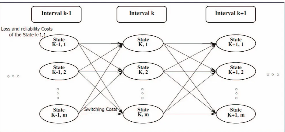
Dynamic Programming Algorithm (DPA) has many advantages for solving a problem that the chief advantage of DPA is reduction in dimensionality of a problem. Assume a year is divided into n periods and the optimal configuration of a network should be determined over each of those periods. If there are m feasible states (m feasible configurations for a network), each state (configuration) could be an answer over each period, so there will be about (m)n _{paths for a year. Note}

that in this study a feasible state is a configuration in which the network is rural and all loads are supplied. As it can be seen it is a large scale problem, so DPA is used to solute this problem (Fig. 1).

As there are several candidate states for each period with different loss and customer interruption costs, DPA should balance the benefits in system reliability and loss against the costs of switching and determine optimum reconfiguration scheme for a year. In this paper the DPA is set up to run forward in time from the initial period to the final period. In each stage the algorithm determine the path with minimum cost to arrive at each state of a period and other non-optimal paths are removed. So in the next stage, for the next time period the path with minimum cost of each state is determined based on costs calculated in the previous period. The recursive algorithm to calculate the minimum cost is as

cos( , ) min[ cos( , ) cos( 1, : , ) cos( 1, )]

(8)

t t t t

F K I = P K I S+ K− L K I +F K− L

Where F_cost(K,I) is the least total cost to arrive at state (K, I) and P_cost(K,I)is operation costs (loss and interruption costs) for state (K,I). Moreover Scost(K−1,L:K,I) is transition (switching) cost from state (K-1, L) to state (K, I) [13]. State (k, I) is the Ith configuration in period K.

After determining configuration of all periods, it could be seen that some switches are always closed over a year. In other words, just some switches help distribution network

reinforcements to have an optimal configuration. Therefore,

appropriate switches for switching can be determined to develop effective feasible configurations.

V. SOLUTION PROCESS AND DISCUSSION

The proposed method to determine annual feeder reconfiguration consists of two main stages. The presented method is as follows:

First Stage: Effective configurations determination

Step 1) Divide a year into 365 daily periods. Note that if the periods are selected shorter the execution time will be longer. On the other hand, if the periods are selected longer it may result in suboptimal solution.

Step 2) Achieve the optimal feeder configuration for all daily periods independently using PSO algorithm, disregarding switching cost.

Step 3) Develop a matrix that contains all obtained optimal feeder configurations in step 2 and find the active switches that participate in switching operation.

Step 4) Determine the effective feasible configurations based on the active switches.

Step 5) If the number of feasible configurations that were obtained from step 4 is enormous, use data mining technique to decrease the number of feasible configurations

Second Stage: Dynamic Programming Algorithm

Step 6) Divide a year into multiperiods and calculate loss and customer interruption for all effective configurations (that are obtained from step 5) during each periods.

Step 7) Calculate switching costs between configurations. Step 8) Run DPA to determine annual reconfiguration scheme. A. PSO algorithm

Population based optimization algorithms, such as PSO and GA often can find optimal solutions for reconfiguration problem. PSO is adopted in this paper to find the optimal

configuration of each period independently. The method that

is used for this purpose is like [5]. The objective function is to minimize total cost of energy loss and customer interruption for each interval

Minimize

C x

( )

=

CLOSS CCI

+

(9)

Where C x( ) denotes the total operation cost for a

distribution system in each period.

More details of PSO algorithm can be found in [5].

B. Data mining technique

In real large distribution networks, number of active switches and consequently number of feasible configurations feed to the DPA will be so high that handling of these feasible configurations may be impossible for DPA. Our experience shows that if there are 1000 candidate configurations for 52 weekly periods, the execution time for running DPA will be about 8 hours. Therefore, if the number of feasible configurations that were obtained from step 4 is enormous, data mining technique will be used for solving the problem for reduction in number of possible configurations. A technique of data mining called APRIORI is used here for reduction in number of possible configurations. The main application of the algorithm is in analyzing of market baskets [14]. Based on items bought by customers, the algorithm finds some association rules. Each rule is something like this:

basket, with which probability Y is also in that basket. More details of APRIORI algorithm can be found in [14].

Assume that each network configuration is a bought basket and each normally opened switch is an item in the basket. So based on the configurations matrix that has been developed in step 3, APRIORI algorithm determines many rules about the relationship between switches.

For example assume a rule is obtained as follow:

Support 0.1153 means that switch 19 and 38 have been opened in 11.53% of configurations. Confidence 1.00 means that if switch 38 was opened in a configuration, switch 19 have been opened in that configuration with the probability of 1.00 (surely). In this problem, rules with confidence of 1.00 are used to limit the number of effective configurations. For example the mentioned rule is applied as: if switch 38 is opened in a configuration, consider the configuration as an effective configuration, just if switch 19 is opened in that configuration too. These rules will be applied to problem insofar as problem dimension becomes proper.

VI. NUMERICAL RESULTS

The proposed method was tested on several test systems. Simulation results of a 33-bus distribution system are presented here. The test system has been used in many reconfiguration studies and is shown in Fig. 2. Operation records of a feeder in Iran have been used as a pattern for residential, commercial and industrial annual load curve.

FIG.2.33-bus distribution network with assigned nodes and switches

1 2 4 6 8 10 12 14 16 18 20 22 24 26 28 30 32 34 36 38 40 42 44 46 48 50 52 0

20 40 60 80

weeks

Lo

ad

Commerical Residential Industrial

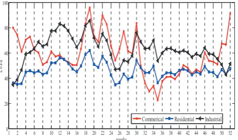
FIG.3.Annual average peak load for commercial, residential and industrial consumers

FIG.4.Average daily load profiles for a typical residential customer during four seasons of a year.

Fig. 3 shows average peak load for commercial, residential and industrial consumers. Moreover, Fig. 4 shows average daily load profiles for a typical residential customer during four seasons of a year. Most of parameter, such as energy, customer interruption and switching cost are borrowed from [12]. The cost of electricity is assumed $6.5625 cents per kWh, the average customer interruption cost for one hour is assumed $0.482, $9.085, and $8.552 per kW for residential, industrial, and commercial customers, respectively. Furthermore, the cost of one switching is assumed $50.75 which is one-eightieth of a new switch installation cost.

At the first step a year is divided into 365 days, then using PSO algorithm, disregarding switching cost, the optimal feeder configurations for all days are obtained. Nine different optimal configurations were obtained that the optimal configuration for all of days was one of these nine configurations. Table I shows these nine configurations. Note that each configuration is shown by its normally open switches.

TABLE I

OPTIMAL CONFIGURATIONS DISREGARDING SWITCHING COST

Configuration Opened switches Configuration Opened switches

1 7-9-13-36-37 6 7-9-14-27-36

2 7-9-14-28-36 7 7-9-14-28-37

3 7-9-14-32-37 8 7-9-13-28-36

4 7-9-14-36-37 9 7-9-14-27-34

TABLE II

FEASIBLE CONFIGURATIONS (STATES OF DP ALGORITHM) Normally opened switches status

1 7-9-13-27-37 9 7-9-14-27-37 17 7-9-27-34-37 2 7-9-13-28-37 10 7-9-14-28-37 18 7-9-28-34-37 3 7-9-13-27-32 11 7-9-14-27-32 19 7-9-27-32-34 4 7-9-13-28-32 12 7-9-14-28-32 20 7-9-28-32-34 5 7-9-13-32-37 13 7-9-14-32-37 21 7-9-32-34-37 6 7-9-13-27-36 14 7-9-14-27-36 22 7-9-27-34-36 7 7-9-13-28-36 15 7-9-14-28-36 23 7-9-28-34-36 8 7-9-13-36-37 16 7-9-14-36-37 24 7-9-34-36-37

TABLE III

FEEDER RECONFIGURATION SCHEDULING USING DPA

Weeks Opened _switches Interruption cost($) Loss Cost ($)

1-4 7-9-14-28-36 4966.44 3456.19

5-10 7-9-14-36-37 20345.24 13411.64

11 7-9-14-28-36 6602.904 4559.693

12-14 7-9-14-36-37 22042.95 14187.14 15-29 7-9-14-28-36 70218.07 46444.73 30-52 7-9-14-32-37 20948.21 30915.65

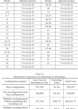
TABLE IV

OPTIMAL CONFIGURATION, DISREGARDING SWITCHING COST

Weeks Opened switches Weeks Opened switches

1 7-9-14-28-36 28-29 7-9-14-28-36

2 7-9-14-36-37 30 7-9-14-32-37

3-4 7-9-14-28-36 31 7-9-14-28-36

5-7 7-9-14-32-37 32-33 7-9-14-32-37

8 7-9-14-28-36 34-35 7-9-14-28-36

9 7-9-14-32-37 36-38 7-9-14-32-37

10 7-9-14-36-37 39-40 7-9-14-28-36

11 7-9-14-28-36 41 7-9-14-32-37

12 7-9-14-32-37 42 7-9-14-17-28

13 7-9-14-36-37 43 7-9-14-28-36

14-15 7-9-14-32-37 44-45 7-9-14-32-37

16-19 7-9-14-28-36 46 7-9-14-28-36

20 7-9-14-32-37 47-48 7-9-14-32-37

21-23 7-9-14-28-36 49 7-9-14-36-37

24 7-9-14-32-37 50 7-9-14-28-32

25 7-9-14-28-36 51 7-9-14-28-36

26 7-9-14-32-37 52 7-9-14-32-37

27 7-9-14-36-37 TABLE V

DIFFERENT CONFIGURATION METHODS COMPARISON

Configuration method _{Interruption Costs} Loss Costs & Switching _Costs Total Costs Base configuration 395,520 No Sw. 395,520 One reconfiguration from

base configuration 260,090 No Sw. 260,090 Multiple reconfigurations

without considering the

switching cost 257,520 2892.75 260,412.75 Multiple reconfigurations

by Dynamic Programming 258,100 304.5 258,404.5

The active switches that participate in switching operation are as below:

S7, S9, S10, S11, S13, S14, S15, S17, S28, S32, S34, S36, S37.

Each feasible configuration of these switches which does not violate technical constraints can be used as one of feasible configurations of DPA for finding annual feeder scheduling. Based on different combination of these active switches 24 feasible configurations are obtained that are shown in Table II. After derivation of feasible configuration from active switches, in next stage a year is divided into 52 weeks. Therefore there will be 24 candidate states for each period. Loss and customer interruption costs for each of the 24 states during all 52 weekly periods are computed. In addition, a matrix with size of 24×24 is developed that each array of that (Ci,j) is the switching cost between configuration i to j using

(5).

After the cost of each state and transition costs between states are determined, using DPA, optimal annual feeder scheduling will be obtained. The simulation results are shown in Table III.

If feeder configurations of 52 weeks being determined without considering the switching cost in feeder scheduling, the result will be as Table IV.

Comparison between results of different reconfiguration scheme is shown in Table V. For the configuration shown in fig. 4, the annual total cost is $395,520. If only one reconfiguration for a whole year is assumed, switches number 7-9-14-28-36 will become normally open switches, and neglecting the switching cost (Table IV), the annual cost will reduce to $260,090. As it can be seen multiple reconfigurations without considering the switching cost results total cost of $260,412.75, which denotes that the switching operation is inappropriate, and reduction in loss and reliability costs may not result in reduction of the total costs. After

executing the procedure proposed in section V, an annual operation cost of $258,404.5 is achievable that is less than other solutions. Comparing the obtained results from third and

fourth rows of this table denotes that it is necessary to compare operation costs consists of system loss, switching costs and reliability costs dynamically to achieve the optimum solution.

VII. CONCLUSION

VIII. REFERENCES

[1] A. Merlin and H. Back, “Search for minimum-loss operating spanning tree configuration in an urban power distribution system,” presented at the Proc. 5th Power System Computation Conference, 1975, Paper 1.2/6. [2] S. Civanlar, J. J. Grainger, H. Yin, and S. S. H. Lee, “Distribution feeder

reconfiguration for loss reduction,” IEEE Trans. Power Del., vol. 3, no. 3, pp. 1217–1223, Jul. 1988.

[3] D. Shirmohammadi, H. Wayne Hong, “Reconfiguration of electric distribution networks for resistive losses reduction”, IEEE Trans. Power Del., vol.4, no. 2, April 1989.

[4] Y. Hong, S. Hu, “Determination of network configuration considering multi-objective in distribution systems using genetic algorithm,” IEEE Trans. Power Syst., vol 20, no 2, pp. 1062–1069, 2005.

[5] X. Jin, J. Zhao, Y. Sun, K. Li and B. Zhang, “Distribution network reconfiguration for load balancing using binary particle swarm optimization,” International conf. power, pp. 507-510, November 2004. [6] Y.-J. Jeon, J.-C. Kim, J.-O. Kim, K. Y. Lee, and J.-R. Shin, “An

efficient simulated annealing algorithm for network reconfiguration in

[7] H. Mori, Y. Ogita, “A parallel tabu search method for reconfiguration of distribution systems,” Proceedings of the 2000 IEEE Power Engineering Society Summer Meeting, vol. 1, pp. 73–78.

[8] A. B. Morton and I. M. Y. Mareels, “An Efficient Brute-Force Solution to the Network Reconfiguration Problem”, IEEE Transactions on Power Delivery, vol. 15. No. 3, pp. 996-1000, July 2000.

[9] R. E. Brown, “Distribution reliability assessment and reconfiguration optimization,” in Proc. Transmission and Distribution Conf. Expo., 2001, vol. 2, pp. 994–999.

[10] Y. Wu, C. Lee, L.C. Liu, “Study of Reconfiguration for the Distribution System with Distributed Generators,” IEEE Trans. Power Del., vol. 25, no. 3, July 2010.

[11] C. S. Chen and M. Y. Cho, “Energy loss reduction by critical switches,” IEEE Trans. Power Del., vol. 8, no. 3, pp. 1246–1253, Jul. 1993. [12] S. A. Yin, C. N. Lu, “Distribution Feeder Scheduling Considering

Variable Load Profile and Outage Costs,” IEEE Trans Power Syst., vol. 24, no. 2, May 2009.

[13] A. J. Wood, B. F. Wollenberg, Power Generation, Operation and Control, vol. 2. New York: Wiley, 1996, p. 131.