The Thirty-Third AAAI Conference on Artificial Intelligence (AAAI-19)
Which Factorization Machine Modeling Is
Better: A Theoretical Answer with Optimal Guarantee
Ming Lin,
1Shuang Qiu,
2Jieping Ye,
2Xiaomin Song,
1Qi Qian,
1Liang Sun,
1Shenghuo Zhu,
1Rong Jin
11Alibaba Group, Bellevue, USA
2Department of Computational Medicine and Bioinformatics, University of Michigan, Ann Arbor, USA {ming.l, xiaomin.song, qi.qian,liang.sun, shenghuo.zhu, jinrong.jr}@alibaba-inc.com,{qiush, jpye}@umich.edu
Abstract
Factorization machine (FM) is a popular machine learning model to capture the second order feature interactions. The optimal learning guarantee of FM and its generalized ver-sion is not yet developed. For a rankkgeneralized FM ofd
dimensional input, the previous best known sampling com-plexity is O[k3d ·polylog(kd)]
under Gaussian distribu-tion. This bound is sub-optimal comparing to the informa-tion theoretical lower boundO(kd). In this work, we aim to tighten this bound towards optimal and generalize the anal-ysis to sub-gaussian distribution. We prove that when the input data satisfies the so-calledτ-Moment Invertible Prop-erty, the sampling complexity of generalized FM can be im-proved toO[k2d·polylog(kd)/τ2]. When the second order self-interaction terms are excluded in the generalized FM, the bound can be improved to the optimalO[kd·polylog(kd)]
up to the logarithmic factors. Our analysis also suggests that the positive semi-definite constraint in the conventional FM is redundant as it does not improve the sampling complexity while making the model difficult to optimize. We evaluate our improved FM model in real-time high precision GPS signal calibration task to validate its superiority.
1
Introduction
Factorization machine (FM) (Rendle 2010; Bayer et al. 2017; Juan, Lefortier, and Chapelle 2017; Juan et al. 2016; Zhao et al. 2017; Yamada et al. 2017; Luo et al. 2018; Lin et al. 2018) is a popular linear regression model to capture the second order feature interactions. It has been found effective in various applications, including recom-mendation systems (Rendle 2010) , CTR prediction (Juan et al. 2016), computational medicine (Lin et al. 2016) , so-cial network (Hong, Doumith, and Davison 2013) and so on. Intuitively speaking, the second order feature interac-tions consider the factors jointly affecting the output. On the theoretical side, FM is closely related to the symmet-ric matrix sensing (Kueng, Rauhut, and Terstiege 2017; Cai and Zhang 2015; Yurtsever et al. 2017) and phase re-trieval (Candes et al. 2013). While the conventional FM only considers the second order feature interactions, it is possible to extend the conventional FM to the high order functional space which leads to the Polynomial Network model (Blon-del et al. 2016). FM is the cornerstone in modern machine
Copyright c2019, Association for the Advancement of Artificial Intelligence (www.aaai.org). All rights reserved.
learning research as it abridges the linear regression and high order polynomial regression. It is therefore important to un-derstand the theoretical foundation of FM.
Given an instancex∈Rd, the conventional FM assumes
that the labely∈Rofxis generated by
y=x>w∗+x>M∗x rank(M∗)≤k (1)
where {w∗, M∗} are the first order and the second order coefficients respectively. In the original FM paper (Rendle 2010), the authors additionally assumed thatM∗ is gener-ated from a low-rank positive semi-definite (PSD) matrix with all its diagonal elements subtracted. That is
M∗=U∗U∗>−diag(U∗U∗>). (2)
Eq. (2) consists of two parts. We call the first partU∗U∗>
as the PSD constraint and the second part−diag(·)as the diagonal-zero constraint. Our key question in this work is whether the FM model (1) can be learned byO[kdlog(kd)] observations and how the two additional constraints help the generalization ability of FM.
Although the FM has been widely applied , there is lit-tle research exploring the theoretical properties of the FM to answer the above key question. A naive analysis directly fol-lowing the sampling complexity of the linear model would suggestO(d2)samples to recover {w∗, M∗}which is too
loose. Whenw∗= 0andM∗is symmetric, Eq. (1) is equal to the symmetric matrix sensing problem. (Cai and Zhang 2015) proved the sampling complexity of this special case on well-bounded sub-gaussian distribution using trace norm convex programming under the`2/`1-RIP condition.
(Yurt-sever et al. 2017) developed a conditional gradient descent solver to recoverM∗. However, whenw∗ 6= 0the above methods and the theoretical results are no longer applica-ble. (Blondel, Fujino, and Ueda 2015) considered a convex-ified formulation of FM. Their FM model requires solving a trace-norm regularized loss function which is computa-tionally expensive. They did not provide statistical learning guarantees for the convexified FM.
of the Gaussian distribution therefore cannot be generalized to non-Gaussian cases. Even limiting on the Gaussian dis-tribution, the sampling complexity given by their analysis is
O[k3d·polylog(kd)]which is worse than the
information-theoretic lower bound O(kd). It is still an open question whether the FM can be learned with O(kd) samples and whether both constraints in the original formulation are nec-essary to make the model learnable.
In this work, we answer the above questions affirma-tively. We show that when the data is sampled from sub-gaussian distribution and satisfies the so-called τ-Moment Invertible Property (MIP), the generalized FM (without con-straints) can be learned byO[k2d/τ2·polylog(kd)]samples.
The PSD constraint is not necessary to achieve this sharp bound. Actually the PSD constraint is harmful as it intro-duces asymmetric bias on the valuey(see Experiment sec-tion). The optimal sampling complexityO[kd·polylog(kd)] is achievable if we further constrain that the diagonal ele-ments ofM∗are zero. This is not an artificial constraint but
there is information-theoretic limitation prevents us recov-ering the diagonal elements of M∗ on sub-gaussian distri-bution. Finally inspired by our theoretical results, we pro-pose an improved version of FM, called iFM, which removes the PSD constraint and inherits the diagonal-zero constraint from the conventional modeling. Unlike the generalized FM, the sampling complexity of the iFM does not depend on the MIP constant of the data distribution.
The remainder of this paper is organized as follows. We revisit the modeling of the FM in Section 2 and show that the conventional modeling is sub-optimal when considered in a more general framework. In Section 3 we present the learn-ing guarantee of the generalized FM on sub-gaussian distri-bution. We propose the high order moment elimination tech-nique to overcome a difficulty in our convergence analysis. Based on our theoretical results, we propose the improved model iFM. Section 4 conducts numerical experiments on synthetic and real-world datasets to validate the superiority of iFM over the conventional FM . Section 5 encloses this work.
2
A Revisit of Factorization Machine
In this section, we revisit the modeling design of the FM and its variants. We briefly review the original formulation of the conventional FM to raise several questions about its optimality. We then highlight previous studies trying to es-tablish the theoretical foundation of the FM modeling. Based on the above survey, we motivate our study and present our main results in the next section.
In their original paper, (Rendle 2010) assumes that the feature interaction coefficients in the FM can be embedded in ak-dimensional latent space. That is,
y= d X
i=1 wixi+
d X
i=1
d X
j=i+1
hui,ujixixj (3)
whereui is a k×1 vector. The original formulation Eq. (3) is equivalent to Eq. (1) with constraint Eq. (2). While the low-rank assumption is standard in the matrix sensing literature, the PSD and the diagonal-zero constraints are not.
A critical question is whether the two additional constraints are necessary or removable. Indeed we have strong reasons to remove both constraints.
The reasons to remove the diagonal-zero constraint are straightforward. First there is no theoretical result so far to motivate this constraint. Secondly subtracting the diagonal elements will make the second order derivative w.r.t.U non-PSD. This will raise many technical difficulties in optimiza-tion and learning theory as many research works assume convexity in their analysis.
The PSD constraint in the original FM modeling is the second term we wish to remove. Let us temporally forget about the diagonal-zero constraint and focus on the PSD constraint only. Obviously relaxing U U> withU V> will make the model more flexible. A more serious problem of the PSD constraint is that it implicitly assumes that the label
yis more likely to be “positive”. This will introduce asym-metric bias about the distribution ofy. To see this, suppose
ˆ
M = U∗U∗> = ¯UΣ ¯U> whereU¯ is the eigenvector ma-trix ofMˆ. We callU¯ the second order feature mapping ma-trix induced byMˆ sincex>Mˆx= ( ¯U>x)>Σ( ¯U>x). The eigenvalue matrixΣis the weights for the mapped features
¯
U>x. AsMˆ is constrained to be PSD, the weights ofU¯>x cannot be negative. In other words, the PSD constraint pre-vents the model learning patterns from negative class. Please check the Experiment section for more concrete examples.
Another issue of the PSD constraint raised is the difficulty in optimization. Suppose we choose least square as the loss function in FM. By enforcing Mˆ = U U>, the loss func-tion is a fourth order polynomial ofU. This makes the ini-tialization ofU difficult since the scale of the initialU(0)
will affect the convergence rate. Clearly we cannot initialize
U(0) = 0 since the gradient w.r.t. U will be zero. On the
other hand, we cannot initializeU(0) to have a large norm
otherwise the problem will be ill-conditioned. This is be-cause the spectral norm of the second order derivative w.r.t.
U will be proportional tokU(0)k2
2therefore the (local)
con-dition number depends onkU(0)k
2. In practice, it is usually
difficult to figure out the optimal scale ofkU(0)k2resulting vanishing or explosion gradient norms. If we decouple the
UandV, we can initializekU(0)k2= 1andV(0)= 0. Then
by alternating gradient descent, the decoupled FM model is easy to optimize.
In summary, the theoretical foundation of the FM is still not well-developed. On one hand, it is unclear whether the conventional FM modeling is optimal and on the other hand, there is strong motivation to modify the conventional formu-lation based on heuristic intuition. This inspires our study of the optimal modeling of the FM driven by theoretical analy-sis which is presented in the next section.
3
Main Results
condition of the data distribution. The sampling complex-ity bound can be improved to optimal by the diagonal-zero constraint.
We introduce a few more notations needed in this sec-tion. Supposex is sampled from coordinate sub-gaussian with zero mean and unit variance. The element-wise third order moment ofxis denoted asκ∗ ,Ex3and the fourth
order moment isφ∗,Ex4. All training instances are
sam-pled identically and independently (i.i.d.). Denote the fea-ture matrix X = [x(1),· · · ,x(n)] ∈
Rd×n and the label
vectory = [y1,· · ·, yn]> ∈ Rn.D(·)denotes the
diago-nal function. For any two matricesAandB, we denote their Hadamard product asA◦B. The element-wise squared ma-trix is defined byA2,A◦A. For a non-negative real num-berξ≥0, the symbolO(ξ)denotes some perturbation ma-trix whose spectral norm is upper bounded byξ. Thei-th largest singular value of matrixM isσi(M). We abbreviate
σ∗i , σi(M∗). To abbreviate our high probability bounds, given a probabilityη, we use the symbolCη andcη to de-note some polynomial logarithmic factors in 1/η and any other necessary variables that do not change the polynomial order of the upper bounds.
3.1
Limitation of The Generalized FM
In order to derive the theoretical optimal FM models, we begin with the most general formulation of FM, that is, with no constraint except low-rank:
y=x>w∗+x>M∗x s.t. M∗=U∗V∗>. (4)
ClearlyM∗ must be symmetric but for now this does not matter. Eq. (4) is called the generalized FM (Lin and Ye 2016). It is proved that whenxis sampled from the Gaussian distribution, Eq. (4) can be learned byO(k3d)training
sam-ples. Although this bound is not optimal, (Lin and Ye 2016) showed the possibility to remove Eq. (2) on the Gaussian distribution. However, their result no longer holds true on non-Gaussian distributions. In the following, we will show that the learning guarantee for the generalized FM on sub-gaussian distribution is much more complex than the Gaus-sian one.
Our first important observation is that model (4) is not always learnable on all sub-gaussian distributions.
Proposition 1. Whenx∈ {−1,+1}d, the generalized FM is not learnable.
The above observation is easy to verify sincex>M∗x=
tr(M∗)whenx∈ {−1,+1}d. Therefore at least the diag-onal elements ofM∗ cannot be recovered at all. Proposi-tion 1 shows that there is informaProposi-tion-theoretic limitaProposi-tion to learn the generalized FM on sub-gaussian distribution. In our analysis, we find that such limitation is related to a property of the data distribution which we call theMoment
Invertible Property (MIP).
Definition 2 (Moment Invertible Property). A zero mean unit variance sub-gaussian distribution P(x) is called τ
-Moment Invertible if|φ−1−κ2| ≥ τfor some constants
τ≥0,φ,Ex4,κ,Ex3.
With the MIP condition, the following theorem shows that the generalized FM is learnable via alternating gradient de-scent.
Theorem 3. Suppose x is sampled from a τ-MIP
sub-gaussian distribution withygenerated by Eq. (4). Then with
probability at least1−η, there is an alternating gradient
descent based method which can achieve the recovery error
aftertiteration such that
kw(t)−w∗k2+kM(t)−M∗k2≤
[(2√5σ1∗/σ∗k+ 2)δ]t(kw∗k2+kM∗k2),
provided
n≥Cη δ2(p+ 1)
2max{pτ−2,(√k+|tr(M)|/kMk2)2d}
p,max{1,kκ∗k∞,kφ∗−3k∞,kφ∗−1k∞}
δ≤min{ 1
2√5σ∗ 1/σk∗+ 2
, 1 2√5σ
∗
k[kw∗k2+kM∗k2]−1}.
Theorem 3 is our key result. In Theorem 3, we measure the quality of our estimation by the recovery error
t,kw(t)−w∗k2+kM(t)−M∗k2.
The recovery error decreases linearly along the steps of alter-nating iteration with rateδ≈ O(1/√n). The sampling com-plexity is on order ofmax{O(k2d},O(1/τ2)}. This bound
delivers two messages. First when the distribution is close to the Gaussian distribution,τ≈2and the bound is controlled byO(k2d). This result improves the previousO(k3d)given by (Lin and Ye 2016) for the Gaussian distribution. Secondly whenτis small, the sampling complexity is proportional to
O(1/τ2). The sampling complexity will even trend to
infi-nite when the data follows the binary Bernoulli distribution whereτ = 0. Therefore theτ-MIP condition provides a suf-ficient condition to make the generalized FM learnable.
We have not given any detail about the alternating gra-dient descent algorithm mentioned in Theorem 3. We find that it is difficult to prove the convergence rate following the conventional alternating gradient descent framework. To ad-dress this difficulty, we use a high order moment elimination technique in the next subsection in the convergent analysis.
3.2
Alternating Gradient Descent with High
Order Moment Elimination
In this subsection, we will construct an alternating gradi-ent descgradi-ent algorithm which achieves the convergence rate and the sampling complexity in Theorem 3. We first show that the conventional alternating gradient descent cannot be applied directly to prove Theorem 3. Then a high order mo-ment elimination technique is proposed to overcome the dif-ficulty.
The generalized FM defined in Eq. (4) can be written in the matrix form
y=X>w∗+A(M∗) (5)
where the operator A(·) : Rd×d → Rd is defined by
Algorithm 1Alternating Gradient Descent with High Order Moment Elimination
Require: The mini-batch size n; number of total update
T; training instancesX(t)
,[x(t,1),x(t,2),· · · ,x(t,n)],
y(t)
,[y(t,1), y(t,2),· · ·, y(t,n)]>; rankk≥1.
Ensure: w(T), U(T), V(T), M(t)
,U(t)V(t)>.
1: Retrieve ntraining instances to estimate the third and fourth order momentsκandφ.
2: ComputeGandHin Eq. (8) and (9).
3: Initialize w(0) = 0, V(0) = 0. U¯(0) =
SVD(M(0)(y(0)), k), that is the top-ksingular vectors.
4: fort= 1,2,· · · , T do
5: Retrieve n training instances X(t),y(t) , compute
M(t)in Eq. (7) and updateU(t)andV(t)as:
ˆ
y(t)=X(t)>w(t−1)+A(t)(U(t−1)V(t−1)>)
U(t)=V(t−1)− M(t)(ˆy(t)
−y(t)) ¯U(t−1)
{U¯(t), R(t)}= QR(U(t))
V(t)=V(t−1)U¯(t−1)>U¯(t)− M(t)(ˆy(t)
−y(t)) ¯U(t)
6: Compute W(t) in Eq. (10) and update w(t) =
w(t−1)− W(t)(ˆy(t)
−y(t)).
7: end for
8: Output:w(T),U¯(T), V(T).
operator of A isA0. To recover {w∗, M∗}, we minimize
the square loss function
min
w,U,V L(w, U, V), 1 2nkX
>w+A(U V>)−yk2. (6)
A straightforward idea to prove Theorem 3 is to show that the alternating gradient descent will converge. However, we find that this is difficult in our problem. To see this, let us compute the expected gradient ofL(w(t), U(t), V(t))with
respect toV(t)at stept.
E∇VL(w(t), U(t), V(t)) =2(M(t)−M∗)U(t)+F(t)U(t) where
F(t),tr(M(t)−M∗)I+D(φ−3)D(M(t)−M∗)
+D(κ)D(w(t)−w∗).
In previous studies, one expectsE∇L ≈I. However, this is
no longer the case in our problem. Clearlyk1
2E∇L −Ik2
is dominated bykκk∞ andkφ−3k∞ . For non-Gaussian distributions, these two perturbation terms could dominate the gradient norm. Similarly the gradient ofwis biased by
O(kκk∞).
The difficulty to follow the conventional gradient descent analysis inspires us to look for a new convergence analysis technique. The perturbation termF(t)consists of high order
moments of the sub-gaussian variablex. It might be possi-ble to construct a sequence of another high order moments to eliminate these perturbation terms. We call this idea the high order moment elimination method. The next question
is whether the desired moments exist and how to construct them efficiently. Unfortunately, this is impossible in general. A sufficient condition to ensure the existence of the elimina-tion sequence is that the data distribuelimina-tion satisfies theτ-MIP condition.
To construction an elimination sequence, for anyz ∈Rn
andM ∈Rd×d, define functions
P(t,0)(z)
,1>z/n, P(t,1)(z)
,X(t)z/n P(t,2)(z)
,(X(t))2z/n− P(t,0)(z) A(t)(M)
,D(X(t)>M X(t))
H(t)(z)
,A(t)0A(t)(z)/(2n).
Notice whenn→ ∞,
P(t,0)(ˆy(t)−y(t))≈tr(M(t)−M∗)
P(t,1)(ˆy(t)
−y(t))≈D(M(t)−M∗)κ+w(t)−w∗
P(t,2)(ˆy(t)
−y(t))≈D(M(t)−M∗)(φ−1)
+D(κ)(w(t)−w∗).
This inspires us to find a linear combination ofP(t,·)to
elim-inateF(t). The solution for this linear combination equation
is
M(t)(ˆy(t)
−y(t)),H(t)(ˆy(t)
−y(t)) (7)
−1
2D
G1◦ P(t,1)(ˆy(t)−y(t))
−1
2D
G2◦ P(t,2)(ˆy(t)−y(t))
where
Gj,:>=
1 κj κj φj−1
−1
κj φj−3
(8)
Hj,:>=
1 κj κj φj−1
−1 1 0
. (9)
Similarly to eliminate the high order moments in the gradi-ent ofw(t), we construct
W(t)(ˆy(t)
−y(t)),H1◦ P(t,1)(ˆy(t)−y(t)) (10)
+H2◦ P(t,2)(ˆy(t)−y(t)).
The overall construction is given in Algorithm 1.
We briefly prove that the construction in Algorithm 1 will eliminate the high order moments in F(t) by which
a global linear convergence rate is immediately followed. Please check appendix for details. We will omit the super-script(t)inX(t)andP(t,·)when not raising confusion.
First we show that n1A0Ais conditionally independent
re-strict isometric after shifting its expectation (Shift CI-RIP). The proof can be found in appendix.
Theorem 4(Shift CI-RIP). Supposed≥(2+kφ∗−3k∞)2.
Fixed a rank-kmatrixM, with probability at least1−η,
1 nA
0A(M) =2M+ tr(M)I+D(φ∗−3)D(M)
+O(δkMk2)
Theorem 4 is the main theorem in our analysis. The key ingredient of our proof is to apply the matrix Bern-stein’s inequality with an improved version of sub-gaussian Hanson-Wright inequality proved by (Rudelson and Ver-shynin 2013). Please check appendix for more details.
Based on the shifted CI-RIP condition of operatorA, we prove the following perturbation bounds.
Lemma 5. Forn≥Cη(
√
k+|tr(M)|)2d/δ2, with
proba-bility at least1−η,
1 nA
0(X>w) =D(κ∗)w+O(δkwk2)
P(0)(y)
,n11>y= tr(M) +O[δ(kwk2+kMk2)]
P(1)(y)
,n1Xy=D(M)κ∗+w+O[δ(kwk2+kMk2)]
P(2)(y)
,n1X2y− P(0)(y) =D(M)(φ∗−1)
+D(κ∗)w+O[δ(kwk2+kMk2)].
Lemma 5 shows thatA0X>andP(t,·)are all concentrated
around their expectations with no more thanO(Cηk2d) sam-ples. To finish our construction, we need to bound the devi-ation ofGandH from their expectationG∗andH∗. This is done in the following lemma.
Lemma 6. Suppose the distribution ofxisτ-MIP withτ > 0. Then in Algorithm 1,
kG−G∗k∞≤δ, kH−H∗k∞≤δ ,
provided
n≥Cη(1 +τ−1 q
kκ∗k2 ∞+kφ
∗ −3k2
∞)/(τ δ 2).
Lemma 6 shows thatG≈G∗ as long asn≥ O(1/τ2).
The matrix inversion in the definition ofGrequires that the
τ-MIP condition must be satisfied withτ >0.
We are now ready to show thatM(t)andW(t)are almost
isometric.
Lemma 7. Under the same settings of Theorem 3, with
probability at least1−η,
M(t)(ˆy(t)−y(t)) =M(t−1)−M∗+O(δt−1)
W(t)(ˆy(t)
−y(t)) =w(t−1)−w∗+O(δt−1)
provided
n≥Cη(p+ 1)2/δ2max{p/τ2,(
√
k+|tr(M)|/kMk2)2d}
wherep,max{1,kκ∗k∞,kφ∗−3k∞,kφ∗−1k∞}.
Lemma 7 shows thatM(t)andW(t)are almost
isomet-ric when the number of samples is larger thanO(k2d)and O(1/τ2). The proof of Lemma 7 consists of two steps. First
we replace each operator or matrix with its expectation plus a small perturbation given in Lemma 5 and Lemma 6. Then Lemma 7 follows after simplification. Theorem 3 is obtained by combining Lemma 7 with alternating gradient descent analysis. Please check appendix for the complete proof.
3.3
Improved Factorization Machine
Theorem 3 shows that learning the generalized FM is hard on non-gaussian distribution. Especially, when the data dis-tribution has a very small τ-MIP constant, the sampling complexity to recover M∗ in Eq. (4) will be as large as
O(1/τ2). The recovery is even impossible onτ = 0 dis-tributions such as the Bernoulli distribution. Clearly, a well-defined learnable model should not depend on the τ-MIP condition.
Indeed the bound given by Theorem 3 is quite sharp. It explains well why we cannot recoverM∗ on the Bernoulli distribution. Therefore it is unlikely to remove theτ depen-dency by designing a better elimination sequence in Algo-rithm 1. After examining the proof of Theorem 1 carefully, we find that the only reason our bound containsτis that the diagonal elements ofM∗are allowed to be non-zero. If we constrainD(M∗) = 0andD(M(t)) = 0, theF(t) in the
expected gradientE∇VL(w(t), U(t), V(t))will be zero and then we do not need to eliminate it during the alternating it-eration. This greatly simplifies our convergence analysis as we only need Theorem 4 which now becomes
1 nA
0A(M) =2M+O(δkMk2). (11)
Eq. (4) already shows that n1A0A is almost isometric that
immediately implies the linear convergence rate of alternat-ing gradient descent. As a direct corollary of Theorem 4, the sampling complexity could be improved toO(cηkd)which is optimal up to some logarithmic constantscη. Inspired by these observations, we propose to learn the following FM model
y=x>w∗+x>M∗x (12)
s.t. M∗=U∗V∗>− D(U∗V∗>).
We called the above model the Improved Factorization Ma-chine (iFM). The iFM model is a trade-off between the con-ventional FM model and the generalized FM model. It de-couples the PSD constraint withU 6=V in the generalized FM model but keeps the diagonal-zero constraint as the con-ventional FM model. Unlike the concon-ventional FM model, the iFM model is proposed in a theoretical-driven way. The de-coupling of{U, V}makes the iFM easy to optimize while the diagonal-zero constraint makes it learnable with the opti-malO(kd)sampling complexity. In the next section, we will verify the above discussion with numerical experiments.
4
Experiments
We first use synthetic data in subsection 4.1 to show the modeling power of iFM and the PSD bias of the conven-tional FM. In subsection 4.2 we apply iFM in a real-word problem, the vTEC estimation task, to demonstrate its supe-riority over baseline methods.
4.1
Synthetic Data
In this subsection, we construct numerical examples to sup-port our theoretical results. To this end, we choosed= 100,
5 10 15 steps
0.025 0.050 0.075 0.100 0.125
RMSE
iFM FM
(a)M∗=U∗U∗>−diag(U∗U∗>)
5 10 15
steps 0.025
0.050 0.075 0.100 0.125
RMSE
iFM FM
(b) inverse the labelyin (a)
5 10 15
steps 0.00
0.02 0.04 0.06 0.08 0.10
RMSE
iFM FM
(c)M∗=U∗V∗>−diag(U∗V∗>)
Figure 1: RMSE Curve of iFM v.s. FM
distribution with variance1/d. We randomly sample 30kd
instances as training set and10000instances as testing set. In Figure 1, we report the convergence curve of iFM and FM on the testing set averaged over 10 trials. The x-axis is the iteration step and the y-axis is the Root Mean Square Error (RMSE) ofy. In Figure (a), we generate labely fol-lowing the conventional FM assumption. Both iFM and FM converge well. In Figure (b), we flip the sign of the label in (a). While iFM still converges well, FM cannot model the sign flip. This example shows why we should avoid to use the conventional FM both in theory and in practice: even a simple flipping operation can make the model under-fit the data. In Figure (c), we generateyfromM∗ with both pos-itive eigenvalues and negative eigenvalues. Again the con-ventional FM cannot fit this data as the distribution ofy is now symmetric in both direction.
4.2
vTEC Estimation
In this subsection, we demonstrate the superiority of iFM in a real-world application, thevertical Total Electron Con-tent(vTEC) estimation. The vTEC is an important descrip-tive parameter of the ionosphere of the Earth. It integrates the total number of electrons integrated when traveling from space to earth with a perpendicular path. One important ap-plication is the real-time high precision GPS signal calibra-tion. The accuracy of the GPS system heavily depends on the pseudo-range measurement between the satellite and the receiver. The major error in the pseudo-range measurement is caused by the vTEC which is dynamic.
In order to estimate the vTEC, we build a triangle mesh grid system in an anonymous region. Each node in the grid is a ground stations equipped with dual-frequency high pre-cision GPS receiver. The distance between two nodes is around 75 kilometers. The station sends out resolved GPS data every second. Formally, our system solves an online regression problem. Our system receivesNtdata points at every time step t measured in seconds. Each data point x(t,i) ∈
R4 presents an ionospheric pierce point of a
satellite-receiver pair. The first two dimensions are the lat-itudeα(t,i)and the longitudeβ(t,i)of the pierce point. The
third dimension and the fourth dimension are the zenith an-gleθ(t,i)and the azimuth angleγ(t,i)respectively. We will
omit the superscriptt below as we always stay within the
same time window t. In order to build a localized predic-tion model, we encode{α(i), β(i)}into a high dimensional
vector. Suppose we havemsatellites in total. First we col-lect data points for 60 seconds. Then we cluster the colcol-lected
{α(i), β(i)}intomclusters via K-means algorithm. Denote
the cluster center of K-means as{c(1),c(2),· · · ,c(m)}and
thei-th data point belongs to thegi-th cluster. The first two dimensions of the i-th data point{α(i), β(i)} are then
en-coded asv(i)∈R2mwhere
v(ji)=
{α(i), β(i)} −c(gi) j=g
i
0 otherwise
Finally, each data pointx(i)is encoded into an
R2m+8
vec-tor:
Enc(x(i)),[v(i),sin(θ(i)),cos(θ(i)), θ(i),(θ(i))2,
sin(γ(i)),cos(γ(i)), γ(i),(γ(i))2].
Evaluation It is important to note that our problem does not fit the conventional machine learning framework. We only have validation set for model selection and evaluation set to evaluate the model performance. We introduce the training station and the testing station that correspond to the “training set” and “testing set” in the conventional machine learning framework. However please be advised that they are not exactly the same concepts.
To evaluate the performance of our models, we randomly select one ground station as the testing station. Around the testing station, we choose16ground stations as training sta-tions to learn the online prediction model. Suppose the on-line prediction model isFwhich mapsEnc(x(i))to the
cor-responding vTEC value
F: Enc(x(i))→vTEC(x(i))∈R.
In our system, we are only given the double difference of thevTECvalues due to the signal resolving process. Sup-pose two satellitesa, band two ground stationsc, dare con-nected in the data-link graph,x(a,c)denotes the ionospheric pierce point between aandc. The observed double differ-encey(a,b,c,d)is given by
y(a,b,c,d),vTEC(x(a,c))−vTEC(x(a,d))−vTEC(x(b,c))
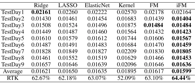
Table 1: RMSE & RTK of iFM v.s. Baseline Methods
Ridge LASSO ElasticNet Kernel FM iFM
TestDay1 0.02161 0.02260 0.02222 0.02570 0.02178 0.02164
TestDay2 0.01430 0.01461 0.01454 0.01683 0.01439 0.01404
TestDay3 0.01508 0.01524 0.01496 0.01875 0.01484 0.01484
TestDay4 0.01449 0.01487 0.01460 0.01564 0.01432 0.01423
TestDay5 0.01610 0.01579 0.01612 0.01744 0.01606 0.01567
TestDay6 0.01487 0.01491 0.01483 0.01684 0.01470 0.01459
TestDay7 0.01828 0.01849 0.01827 0.02209 0.01830 0.01805
TestDay8 0.01461 0.01552 0.01519 0.01629 0.01466 0.01453
TestDay9 0.01657 0.01646 0.01639 0.02096 0.01646 0.01636
Average 0.01621 0.01650 0.01635 0.01895 0.01617 0.01599
RTK 62.67% 62.18% 63.07% 52.09% 63.10% 64.44%
SincevTEC(·)is an unknown function, we need to approx-imate it byF. OnceFis learned from training stations, we can apply it to predict the double differencey(a,b,c,d)where eithercordis the testing station.
Once we get the vTEC estimation, we use it to calibrate the GPS signal and finally compute the geometric coordi-nate of the user. The RTK ratio measures the quality of the positioning service. It is a real number presenting the prob-ability of successful positioning with accuracy at least one centimeter. The RTK ratio is computed from a commercial system that is much slower than the computation of RMSE.
Dataset and Results We select a ground station at the re-gion center as testing station. Around the testing station 16 stations are selected as training stations. We collect 5 con-secutive days’ data as validation set for parameter tuning. The following 9 days’ data are used as evaluation set. We up-date the prediction model per 60 seconds. The learned model is then used to predict the double differences relating to the testing station. We compare the predicted double differences to the true values detected by the testing station. The number of valid satellites in our experiment is around 10 to 20.
In Table 1, we report the root-mean-square error (RMSE) over 9 days period. The dates are denoted as TestDay1 to TestDay9 for anonymity. Five baseline methods are evalu-ated: Ridge Regression, LASSO, ElasticNet, Kernel Ridge Regression (Kernel) with RBF kernel and the conventional Factorization Machine (FM). More computational expensive models such as deep neural network are not feasible for our online system. For Ridge, LASSO, Kernel and ElasticNet, their parameters are tuned from1×10−6to1×106. The
reg-ularizer parameters of FM and iFM are tuned from1×10−6 to1×106. The rank ofM is tuned in set{1,2,· · ·,10}. We
use Scikit-learn (Pedregosa et al. 2011) and fastFM (Bayer 2016) to implement the baseline methods.
In Table 1, we observe that iFM is uniformly better than the baseline methods. We average the root squared error over 9×24×60 = 12960minutes in the last second row. The 95% confidence interval is within1×10−5in our experiment. In our experiment, the optimal rank of FM is 2 and the optimal rank of iFM is 6. We note that FM is better than the first order linear models since it captures the second order information.
This indicates that the second order information is indeed helpful.
In the last row of Table 1, we report the RTK ratio aver-aged over the 9 days. We find that the RTK ratio will improve a lot even with small improvement of vTEC estimation. This is because the error of vTEC estimation will be broadcasted and magnified in the RTK computation pipeline. The RTK ratio of iFM is about 1.77% better than that of Ridge regres-sion and is more than 12% better than Kernel regresregres-sion. Comparing to FM, it is 1.34% better. We conclude that iFM achieves overall better performance and the improvement is statistically significant.
5
Conclusion
We study the learning guarantees of the FM solved by al-ternating gradient descent on sub-gaussian distributions. We find that the conventional modeling of the factorization ma-chine might be sub-optimal in capturing negative second or-der patterns. We prove that the constraints in the conven-tional FM can be removed resulting a generalized FM model learnable by max{O(k2d},O(1/τ2)} samples. The
sam-pling complexity can be improved to the optimalO(kd)with diagonal-zero constraint. Our theoretical analysis shows that the optimal modeling of high order linear model does not al-ways agree with the heuristic intuition. We hope this work could inspire future researches of non-convex high order machines with solid theoretical foundation.
6
Acknowledgments
This research is supported in part by NSF (III-1539991). The high precision GPS dataset is provided by Qianxun Spa-tial Intelligence Inc. China. We appreciate Dr. Wotao Yin from University of California Los Angeles and anonymous reviewers for their insightful comments.
References
Bayer, I.; He, X.; Kanagal, B.; and Rendle, S. 2017. A generic coordinate descent framework for learning from im-plicit feedback. In Proceedings of the 26th International
Bayer, I. 2016. fastFM: A Library for Factorization Ma-chines. Journal of Machine Learning Research17(184):1– 5.
Blondel, M.; Ishihata, M.; Fujino, A.; and Ueda, N. 2016. Polynomial Networks and Factorization Machines: New In-sights and Efficient Training Algorithms. InProceedings of
The 33rd International Conference on Machine Learning,
850–858.
Blondel, M.; Fujino, A.; and Ueda, N. 2015. Convex Fac-torization Machines. InMachine Learning and Knowledge
Discovery in Databases, number 9285 in Lecture Notes in
Computer Science.
Cai, T. T., and Zhang, A. 2015. ROP: Matrix recovery via rank-one projections. The Annals of Statistics43(1):102– 138.
Candes, E.; Eldar, Y.; Strohmer, T.; and Voroninski, V. 2013. Phase Retrieval via Matrix Completion. SIAM Journal on
Imaging Sciences6(1):199–225.
Hong, L.; Doumith, A. S.; and Davison, B. D. 2013. Co-factorization Machines: Modeling User Interests and Pre-dicting Individual Decisions in Twitter. InProceedings of the Sixth ACM International Conference on Web Search and
Data Mining, 557–566.
Juan, Y.; Zhuang, Y.; Chin, W.-S.; and Lin, C.-J. 2016. Field-aware Factorization Machines for CTR Prediction. In Pro-ceedings of the 10th ACM Conference on Recommender Sys-tems, 43–50.
Juan, Y.; Lefortier, D.; and Chapelle, O. 2017. Field-aware factorization machines in a real-world online advertising system. InProceedings of the 26th International
Confer-ence on World Wide Web Companion, WWW ’17
Compan-ion, 680–688.
Kueng, R.; Rauhut, H.; and Terstiege, U. 2017. Low rank matrix recovery from rank one measurements. Applied and
Computational Harmonic Analysis42(1):88–116.
Lin, M., and Ye, J. 2016. A non-convex one-pass framework for generalized factorization machine and rank-one matrix sensing. InAdvances in Neural Information Processing Sys-tems, 1633–1641.
Lin, K.; Xu, J.; Baytas, I. M.; Ji, S.; and Zhou, J. 2016. Multi-Task Feature Interaction Learning. In Proceedings of the 22Nd ACM SIGKDD International Conference on
Knowledge Discovery and Data Mining, 1735–1744.
Lin, X.; Zhang, W.; Zhang, M.; Zhu, W.; Pei, J.; Zhao, P.; and Huang, J. 2018. Online compact convexified factoriza-tion machine. InProceedings of the 2018 World Wide Web
Conference on World Wide Web, 1633–1642.
Luo, L.; Zhang, W.; Zhang, Z.; Zhu, W.; Zhang, T.; and Pei, J. 2018. Sketched follow-the-regularized-leader for on-line factorization machine. InProceedings of the 24th ACM SIGKDD International Conference on Knowledge
Discov-ery & Data Mining, 1900–1909.
Pedregosa, F.; Varoquaux, G.; Gramfort, A.; Michel, V.; Thirion, B.; Grisel, O.; Blondel, M.; Prettenhofer, P.; Weiss, R.; Dubourg, V.; Vanderplas, J.; Passos, A.; Cournapeau, D.;
Brucher, M.; Perrot, M.; and Duchesnay, E. 2011. Scikit-learn: Machine learning in Python. Journal of Machine
Learning Research12:2825–2830.
Rendle, S. 2010. Factorization machines. In IEEE 10th
International Conference On Data Mining, 995–1000.
Roman Vershynin. 2017. High-Dimensional Probability:
An Introduction with Applications in Data Science.
Rudelson, M., and Vershynin, R. 2013. Hanson-Wright in-equality and sub-gaussian concentration. Electronic
Com-munications in Probability18.
Stewart, G. W., and Sun, J.-g. 1990. Matrix Perturbation
Theory. Boston: Academic Press, 1 edition edition.
Tao, T. 2012.Topics in Random Matrix Theory, volume 132. Amer Mathematical Society.
Yamada, M.; Lian, W.; Goyal, A.; Chen, J.; Wimalawarne, K.; Khan, S. A.; Kaski, S.; Mamitsuka, H.; and Chang, Y. 2017. Convex factorization machine for toxicogenomics prediction. InProceedings of the 23rd ACM SIGKDD In-ternational Conference on Knowledge Discovery and Data
Mining, 1215–1224.
Yurtsever, A.; Udell, M.; Tropp, J. A.; and Cevher, V. 2017. Sketchy Decisions: Convex Low-Rank Matrix Optimization with Optimal Storage. arXiv:1702.06838 [math, stat]. Zhao, H.; Yao, Q.; Li, J.; Song, Y.; and Lee, D. L. 2017. Meta-graph based recommendation fusion over heteroge-neous information networks. In Proceedings of the 23rd ACM SIGKDD International Conference on Knowledge