Scalable Influence Maximization for Multiple Products in
Continuous-Time Diffusion Networks
Nan Du [email protected]
Google Research, 1600 Amphitheatre Pkwy, Mountain View, CA 94043
Yingyu Liang [email protected]
Department of Computer Science, Princeton University, Princeton, NJ 08540
Maria-Florina Balcan [email protected]
School of Computer Science, Carnegie Mellon University, Pittsburgh, PA 15213
Manuel Gomez-Rodriguez [email protected]
MPI for Software Systems, Kaiserslautern, Germany 67663
Hongyuan Zha [email protected]
Le Song [email protected]
College of Computing, Georgia Institute of Technology, Atlanta, GA 30332
Editor:Jeff Bilmes
Abstract
A typical viral marketing model identifies influential users in a social network to maxi-mize a single product adoption assuming unlimited user attention, campaign budgets, and time. In reality, multiple products need campaigns, users have limited attention, convinc-ing users incurs costs, and advertisers have limited budgets and expect the adoptions to be maximized soon. Facing these user, monetary, and timing constraints, we formulate the problem as a submodular maximization task in a continuous-time diffusion model under the intersection of one matroid and multiple knapsack constraints. We propose a randomized algorithm estimating the user influence1in a network (|V|nodes,|E|edges) to an accuracy
ofwithn=O(1/2) randomizations and ˜O(n|E|+n|V|) computations. By exploiting the
influence estimation algorithm as a subroutine, we develop an adaptive threshold greedy algorithm achieving an approximation factor ka/(2 + 2k) of the optimal when ka out of
the k knapsack constraints are active. Extensive experiments on networks of millions of nodes demonstrate that the proposed algorithms achieve the state-of-the-art in terms of effectiveness and scalability.
Keywords: Influence Maximization, Influence Estimation, Continuous-time Diffusion Model, Matroid, Knapsack
1. Introduction
Online social networks play an important role in the promotion of new products, the spread of news, the success of political campaigns, and the diffusion of technological innovations. In these contexts, the influence maximization problem (or viral marketing problem) typically
1. Partial results in the paper on influence estimation have been published in a conference paper: Nan Du, Le Song, Manuel Gomez-Rodriguez, and Hongyuan Zha. Scalable influence estimation in continuous time diffusion networks. In Advances in Neural Information Processing Systems 26, 2013.
c
has the following flavor: identify a set of influential users in a social network, who, when convinced to adopt a product, shall influence other users in the network and trigger a large cascade of adoptions. This problem has been studied extensively in the literature from both the modeling and the algorithmic aspects (Richardson and Domingos, 2002; Kempe et al., 2003; Leskovec et al., 2007; Chen et al., 2009, 2010a,b, 2011, 2012; Ienco et al., 2010; Goyal et al., 2011a,b; Gomez-Rodriguez and Sch¨olkopf, 2012), where it has been typically assumed that the host (e.g., the owner of an online social platform) faces a single product, endless user attention, unlimited budgets and unbounded time. However, in reality, the host often encounters a much more constrained scenario:
• Multiple-Item Constraints: multiple products can spread simultaneously among the same set of social entities. These products may have different characteristics, such as their revenues and speed of spread.
• Timing Constraints: the advertisers expect the influence to occur within a certain time window, and different products may have different timing requirements.
• User Constraints: users of the social network, each of which can be a potential source, would like to be exposed to only a small number of ads. Furthermore, users may be grouped by their geographical locations, and advertisers may have a target population they want to reach.
• Product Constraints: seeking initial adopters entails a cost to the advertiser, who needs to pay to the host and often has a limited amount of money.
For example, Facebook (i.e., the host) needs to allocate ads for various products with different characteristics, e.g., clothes, books, or cosmetics. While some products, such as clothes, aim at influencing within a short time window, some others, such as books, may allow for longer periods. Moreover, Facebook limits the number of ads in each user’s side-bar (typically it shows less than five) and, as a consequence, it cannot assign all ads to a few highly influential users. Finally, each advertiser has a limited budget to pay for ads on Facebook and thus each ad can only be displayed to some subset of users. In our work, we incorporate these myriads of practical and important requirements into consideration in the influence maximization problem.
We account for the multi-product and timing constraints by applying product-specific continuous-time diffusion models. Here, we opt for continuous-time diffusion models in-stead of discrete-time models, which have been mostly used in previous work (Kempe et al., 2003; Chen et al., 2009, 2010a,b, 2011, 2012; Borgs et al., 2012). This is because arti-ficially discretizing the time axis into bins introduces additional errors. One can adjust the additional tuning parameters, like the bin size, to balance the tradeoff between the error and the computational cost, but the parameters are not easy to choose optimally. Extensive experimental comparisons on both synthetic and real-world data have shown that discrete-time models provide less accurate influence estimation than their continuous-time counterparts (Gomez-Rodriguez et al., 2011; Gomez-Rodriguez and Sch¨olkopf, 2012; Gomez-Rodriguez et al., 2013; Du et al., 2013a,b).
problem (i.e., the influence estimation problem) in this setting is a difficult graphical model inference problem, i.e., computing the marginal density of continuous variables in loopy graphical models. The exact answer can be computed only for very special cases. For ex-ample, Gomez-Rodriguez and Sch¨olkopf (2012) have shown that the problem can be solved exactly when the transmission functions are exponential densities, by using continuous time Markov processes theory. However, the computational complexity of such approach, in gen-eral, scales exponentially with the size and density of the network. Moreover, extending the approach to deal with arbitrary transmission functions would require additional nontrivial approximations which would increase even more the computational complexity. Second, it is unclear how to scale up influence estimation and maximization algorithms based on continuous-time diffusion models to millions of nodes. Especially in the maximization case, the influence estimation procedure needs to be called many times for different subsets of selected nodes. Thus, our first goal is to design a scalable algorithm which can perform influence estimation in the regime of networks with millions of nodes.
We account for the user and product constraints by restricting the feasible domain over which the maximization is performed. We first show that the overall influence function of multiple products is a submodular function and then realize that the user and product con-straints correspond to concon-straints over the ground set of this submodular function. To the best of our knowledge, previous work has not considered both user and product constraints simultaneously over general unknown different diffusion networks with non-uniform costs. In particular, (Datta et al., 2010) first tried to model both the product and user constraints only with uniform costs and infinite time window, which essentially reduces to a special case of our formulations. Similarly, (Lu et al., 2013) considered the allocation problem of multiple products which may have competitions within the infinite time window. Be-sides, they all assume that multiple products spread within the same network. In contrast, our formulations generally allow products to have different diffusion networks, which can be unknown in practice. Soma et al. (2014) studied the influence maximization problem for one product subject to one knapsack constraint over a known bipartite graph between marketing channels and potential customers; Ienco et al. (2010) and Sun et al. (2011) con-sidered user constraints but disregarded product constraints during the initial assignment; and, Narayanam and Nanavati (2012) studied the cross-sell phenomenon (the selling of the first product raises the chance of selling the second) and included monetary constraints for all the products. However, no user constraints were considered, and the cost of each user was still uniform for each product. Thus, our second goal is to design an efficient submod-ular maximization algorithm which can take into account both user and product constraints simultaneously.
Overall, this article includes the following major contributions:
• Unlike prior work that considers an a priori described simplistic discrete-time diffu-sion model, we firstlearnthe diffusion networks from data by using continuous-time diffusion models. This allows us to address the timing constraints in a principled way.
• We propose an efficient randomized algorithm for continuous-time influence estima-tion, which can scale up to millions of nodes and estimate the influence of each node to an accuracy ofusing n=O(1/2) randomizations.
• We formulate the influence maximization problem with the aforementioned constraints as a submodular maximization under the intersection of matroid constraints and knap-sack constraints. The submodular function we use is based on the actual diffusion model learned from the data for the time window constraint. This novel formula-tion provides us a firm theoretical foundaformula-tion for designing greedy algorithms with theoretical guarantees.
• We develop an efficient adaptive-threshold greedy algorithm which is linear in the number of products and proportional to Oe(|V|+|E∗|), where |V| is the number of nodes (users) and|E∗|is the number of edges in the largest diffusion network. We then prove that this algorithm is guaranteed to find a solution with an overall influence of at least ka
2+2k of the optimal value, when ka out of the k knapsack constraints
are active. This improves over the best known approximation factor achieved by polynomial time algorithms in the combinatorial optimization literature. Moreover, whenever advertising each product to each user entails the same cost, the constraints reduce to an intersection of matroids, and we obtain an approximation factor of 1/3, which is optimal for such optimization.
• We evaluate our algorithms over large synthetic and real-world datasets and show that our proposed methods significantly improve over previous state-of-the-arts in terms of both the accuracy of the estimated influence and the quality of the selected nodes in maximizing the influence over independently hold-out real testing data.
In the remainder of the paper, we will first tackle the influence estimation problem in section 2. We then formulate different realistic constraints for the influence maximization in section 3 and present the adaptive-thresholding greedy algorithm with its theoretical analysis in section 4; we investigate the performance of the proposed algorithms in both synthetic and real-world datasets in section 5; and finally we conclude in section 6.
2. Influence Estimation
We start by revisiting the continuous-time diffusion model by Gomez-Rodriguez et al. (2011) and then explicitly formulate the influence estimation problem from the perspective of probabilistic graphical models. Because the efficient inference of the influence value for each node is highly non-trivial, we further develop a scalable influence estimation algorithm which is able to handle networks of millions of nodes. The influence estimation procedure will be a key building block for our later influence maximization algorithm.
2.1 Continuous-Time Diffusion Networks
Moreover, it also differs from discrete-time models in the sense that events in a cascade are not generated iteratively in rounds, but event timings are sampled directly from the transmission function in the continuous-time model.
Continuous-Time Independent Cascade Model. Given adirected contact network, G= (V,E), we use the independent cascade model for modeling a diffusion process (Kempe et al., 2003; Gomez-Rodriguez et al., 2011). The process begins with a set of infected source nodes,A, initially adopting certain contagion (idea, meme or product) at time zero. The contagion is transmitted from the sources along their out-going edges to their direct neighbors. Each transmission through an edge entailsrandomwaiting times,τ, drawn from different independent pairwise waiting time distributions(one per edge). Then, the infected neighbors transmit the contagion to their respective neighbors, and the process continues. We assume that an infected node remains infected for the entire diffusion process. Thus, if a node i is infected by multiple neighbors, only the neighbor that first infects node i will be thetrue parent. As a result, although the contact network can be an arbitrary directed network, each diffusion process induces a Directed Acyclic Graph (DAG).
Heterogeneous Transmission Functions. Formally, the pairwise transmission func-tion fji(ti|tj) for a directed edgej →iis the conditional density of node igetting infected
at time ti given that node j was infected at time tj. We assume it is shift invariant: fji(ti|tj) =fji(τji), whereτji:=ti−tj, and causal: fji(τji) = 0 if τji<0. Both parametric
transmission functions, such as the exponential and Rayleigh function (Gomez-Rodriguez et al., 2011), and nonparametric functions (Du et al., 2012) can be used and estimated from cascade data.
Shortest-Path Property. The independent cascade model has a useful property we will use later: given a sample of transmission times of all edges, the timeti taken to infect
a nodeiis the length of the shortest path in G from the sources to nodei, where the edge weights correspond to the associated transmission times.
2.2 Probabilistic Graphical Model for Continuous-Time Diffusion Networks The continuous-time independent cascade model is essentially a directed graphical model for a set of dependent random variables, that is, the infection timesti of the nodes, where the
conditional independence structure is supported on the contact network G. Although the original contact graph G can contain directed loops, each diffusion process (or a cascade) induces a directed acyclic graph (DAG). For those cascades consistent with a particular DAG, we can model the joint density of ti using a directed graphical model:
p({ti}i∈V) = Y
i∈Vp(ti|{tj}j∈πi), (1)
where each πi denotes the collection of parents of node i in the induced DAG, and each
term p(ti|{tj}j∈πi) corresponds to a conditional density of ti given the infection times of the parents of node i. This is true because given the infection times of node i’s parents,ti
However, these conditional densities can be derived from the pairwise transmission func-tions based on the Independent-Infection property:
p(ti|{tj}j∈πi) = X
j∈πi
fji(ti|tj)
Y
l∈πi,l6=j
S(ti|tl), (2)
which is the sum of the likelihoods that node i is infected by each parent node j. More precisely, each term in the summation can be interpreted as the likelihoodfji(ti|tj) of node i being infected at ti by nodej multiplied by the probability S(ti|tl) that it has survived
from the infection of each other parent node l6=j until time ti.
Perhaps surprisingly, the factorization in Equation (1) is the same factorization that can be used for an arbitrary induced DAG consistent with the contact network G. In this case, we only need to replace the definition ofπi (the parent of node iin the DAG) to the
set of neighbors of node i with an edge pointing to node i in G. This is not immediately obvious from Equation (1), since the contact network G can contain directed loops which seems to be in conflict with the conditional independence semantics of directed graphical models. The reason why it is possible to do so is as follows: any fixed set of infection times, t1, . . . , td, induces an ordering of the infection times. If ti ≤ tj for an edge j → i
inG,hji(ti|tj) = 0, and the corresponding term in Equation (2) is zeroed out, making the
conditional density consistent with the semantics of directed graphical models.
Instead of directly modeling the infection times ti, we can focus on the set of mutually
independent random transmission times τji = ti −tj. Interestingly, by switching from a
node-centric view to an edge-centric view, we obtain a fully factorized joint density of the set of transmission times
p {τji}(j,i)∈E
=Y
(j,i)∈Efji(τji), (3) Based on the Shortest-Path property of the independent cascade model, each variabletican
be viewed as a transformation from the collection of variables{τji}(j,i)∈E. More specifically, let Qi be the collection of directed paths inG from the source nodes to nodei, where each
path q ∈ Qi contains a sequence of directed edges (j, l). Assuming all source nodes are infected at time zero, then we obtain variableti via
ti =gi {τji}(j,i)∈E|A
= min
q∈Qi X
(j,l)∈qτjl, (4)
where the transformation gi(·|A) is the value of the shortest-path minimization. As a
special case, we can now compute the probability of nodeiinfected beforeT using a set of independent variables:
Pr{ti≤T|A}= Pr
gi {τji}(j,i)∈E|A
≤T . (5)
2.3 Influence Estimation Problem in Continuous-Time Diffusion Networks Intuitively, given a time window, the wider the spread of infection, the more influential the set of sources. We adopt the definition of influence as the expected number of infected nodes given a set of source nodes and a time window, as in previous work (Gomez-Rodriguez and Sch¨olkopf, 2012). More formally, consider a set of source nodes A ⊆ V,|A| ≤C which get infected at time zero. Then, given a time window T, a node i is infected within the time window if ti ≤T. The expected number of infected nodes (or the influence) given the set
of transmission functions{fji}(j,i)∈E can be computed as
σ(A, T) =E
hX
i∈VI{ti ≤T|A} i
=X
i∈VPr{ti≤T|A}, (6) whereI{·}is the indicator function and the expectation is taken over the the set ofdependent
variables {ti}i∈V. By construction, σ(A, T) is a non-negative, monotonic nondecreasing submodular function in the set of source nodes shown by Gomez-Rodriguez and Sch¨olkopf (2012).
Essentially, the influence estimation problem in Equation (6) is an inference problem for graphical models, where the probability of eventti ≤T given sources inA can be obtained
by summing out the possible configuration of other variables{tj}j6=i. That is
Pr{ti≤T|A}=
Z ∞
0 · · ·
Z T
ti=0 · · ·
Z ∞
0 Y
j∈Vp tj|{tl}l∈πj
Y
j∈Vdtj
, (7)
which is, in general, a very challenging problem. First, the corresponding directed graphical models can contain nodes with high in-degree and high out-degree. For example, in Twitter, a user can follow dozens of other users, and another user can have hundreds of “followers”. The tree-width corresponding to this directed graphical model can be very high, and we need to perform integration for functions involving many continuous variables. Second, the integral in general can not be evaluated analytically for heterogeneous transmission functions, which means that we need to resort to numerical integration by discretizing the domain [0,∞). If we use N levels of discretization for each variable, we would need to enumerate O(N|πi|) entries, exponential in the number of parents.
Only in very special cases, can one derive the closed-form equation for computing Pr{ti≤T|A}. For instance, Gomez-Rodriguez and Sch¨olkopf (2012) proposed an approach
for exponential transmission functions, where the special properties of exponential density are used to map the problem into a continuous time Markov process problem, and the com-putation can be carried out via a matrix exponential. However, without further heuristic approximation, the computational complexity of the algorithm is exponential in the size and density of the network. The intrinsic complexity of the problem entails the utilization of approximation algorithms, such as mean field algorithms or message passing algorithms. We will design an efficient randomized (or sampling) algorithm in the next section.
we can derive the influence function as
σ(A, T) =X
i∈VPr
gi {τji}(j,i)∈E|A
≤T
=E
hX
i∈VI
gi {τji}(j,i)∈E|A
≤T i, (8)
where the expectation is with respect to the set of independent variables{τji}(j,i)∈E. This equivalent formulation suggests a naive sampling (NS) algorithm for approximatingσ(A, T): draw n samples of {τji}(j,i)∈E, run a shortest path algorithm for each sample, and finally average the results (see Appendix A for more details). However, this naive sampling ap-proach has a computational complexity ofO(nC|V||E|+nC|V|2log|V|) due to the repeated calling of the shortest path algorithm. This is quadratic to the network size, and hence not scalable to millions of nodes.
Our second key observation is that for each sample{τji}(j,i)∈E, we are only interested in the neighborhood size of the source nodes,i.e., the summation P
i∈VI{·} in Equation (8), rather than in the individual shortest paths. Fortunately, the neighborhood size estimation problem has been studied in the theoretical computer science literature. Here, we adapt a very efficient randomized algorithm by Cohen (1997) to our influence estimation problem. This randomized algorithm has a computational complexity of O(|E|log|V|+|V|log2|V|) and it estimates the neighborhood sizes for all possible single source node locations. Since it needs to run once for each sample of{τji}(j,i)∈E, we obtain an overall influence estimation algorithm with O(n|E|log|V|+n|V|log2|V|) computation, nearly linear in network size. Next we will revisit Cohen’s algorithm for neighborhood estimation.
2.4.1 Randomized Algorithm for Single-Source Neighborhood-Size Estimation
Given a fixed set of edge transmission times {τji}(j,i)∈E and a source node s, infected at time zero, the neighborhood N(s, T) of a source nodes given a time window T is the set of nodes within distanceT froms,i.e.,
N(s, T) =
i gi {τji}(j,i)∈E
≤T, i∈ V . (9)
Instead of estimatingN(s, T) directly, the algorithm will assign an exponentially distributed random labelrito each network nodei. Then, it makes use of the fact that the minimum of a
set of exponential random variables{ri}i∈N(s,T)is still an exponential random variable, but with its parameter being equal to the total number of variables, that is, if eachri∼exp(−ri),
then the smallest label within distanceT from sources,r∗:= mini∈N(s,T)ri, will distribute
as r∗ ∼exp{−|N(s, T)|r∗}. Suppose we randomize over the labeling m times and obtain m such least labels, {r∗u}mu=1. Then the neighborhood size can be estimated as
|N(s, T)| ≈ Pmm−1
u=1r∗u
. (10)
Cohen (1997) designed a modified Dijkstra’s algorithm (Algorithm 3) to construct a data structurer∗(s), called least label list, for each nodesto support such query. Essentially, the algorithm starts with the nodeiwith the smallest labelri, and then it traverses in
breadth-first search fashion along the reverse direction of the graph edges to find all reachable nodes. For each reachable node s, the distance d∗ between i and s, and ri are added to the end
of r∗(s). Then the algorithm moves to the nodei0 with the second smallest label ri0, and
similarly find all reachable nodes. For each reachable node s, the algorithm will compare the current distance d∗ between i0 and s with the last recorded distance in r∗(s). If the current distance is smaller, then the current d∗ and ri0 are added to the end ofr∗(s). Then
the algorithm move to the node with the third smallest label and so on. The algorithm is summarized in Algorithm 3 in Appendix B.
Algorithm 3 returns a list r∗(s) per node s ∈ V, which contains information about distance to the smallest reachable labels from s. In particular, each list contains pairs of distance and random labels, (d, r), and these pairs are ordered as
∞> d(1)> d(2) > . . . > d(|r∗(s)|)= 0 (11)
r(1)< r(2)< . . . < r(|r∗(s)|), (12)
where{·}(l) denotes the l-th element in the list. (see Appendix B for an example).
If we want to query the smallest reachable random label r∗ for a given source sand a timeT, we only need to perform a binary search on the list for node s:
r∗ =r(l), whered(l−1) > T ≥d(l). (13) Finally, to estimate|N(s, T)|, we generatem i.i.d. collections of random labels, run Algo-rithm 3 on each collection, and obtainm values{ru∗}mu=1, which we use in Equation (10) to estimate |N(i, T)|.
The computational complexity of Algorithm 3 is O(|E|log|V|+|V|log2|V|), with ex-pected size of each r∗(s) being O(log|V|). Then the expected time for querying r∗ is O(log log|V|) using binary search. Since we need to generate m set of random labels and run Algorithm 3 m times, the overall computational complexity for estimating the single-source neighborhood size for all s ∈ V is O(m|E|log|V|+m|V|log2|V|+m|V|log log|V|). For large-scale network, and when m min{|V|,|E|}, this randomized algorithm can be much more efficient than approaches based on directly calculating the shortest paths.
2.4.2 Constructing Estimation for Multiple-Source Neighborhood Size
When we have a set of sources, A, its neighborhood is the union of the neighborhoods of its constituent sources
N(A, T) =[
i∈AN(i, T). (14)
This is true because each source independently infects its downstream nodes. Furthermore, to calculate the least label list r∗ corresponding toN(A, T), we can simply reuse the least label list r∗(i) of each individual source i∈ A. More formally,
where the inner minimization can be carried out by querying r∗(i). Similarly, after we obtain msamples of r∗, we can estimate|N(A, T)|using Equation (10). Importantly, very little additional work is needed when we want to calculate r∗ for a set of sources A, and we can reuse work done for a single source. This is very different from a naive sampling approach where the sampling process needs to be done completely anew if we increase the source set. In contrast, using the randomized algorithm, only an additional constant-time minimization over|A| numbers is needed.
2.4.3 Overall Algorithm
So far, we have achieved efficient neighborhood size estimation of|N(A, T)|with respect to a given set of transmission times{τji}(j,i)∈E. Next, we will estimate the influence by averaging over multiple sets of samples for {τji}(j,i)∈E. More specifically, the relation from (8)
σ(A, T) =E{τji}(j,i)∈E[|N(A, T)|] =E{τji}E{r1,...,rm}|{τji}
m−1
Pm
u=1r∗u
, (16)
suggests the following overall algorithm :
Continuous-Time Influence Estimation (ConTinEst):
1. Samplensets of random transmission times{τijl }(j,i)∈E ∼ Q
(j,i)∈Efji(τji).
2. Given a set of{τijl}(j,i)∈E, samplemsets of random labels{rui}i∈V ∼ Qi∈Vexp(−ri).
3. Estimateσ(A, T) by sample averages σ(A, T)≈ 1
n
Pn
l=1
(m−1)/Pm
ul=1r
ul ∗
.
What is even more important is that the number of random labels, m, does not need to be very large. Since the estimator for |N(A, T)| is unbiased (Cohen, 1997), essentially the outer-loop of averaging over n samples of random transmission times further reduces the variance of the estimator in a rate of O(1/n). In practice, we can use a very small m (e.g., 5 or 10) and still achieve good results, which is also confirmed by our later experi-ments. Compared to (Chen et al., 2009), the novel application of Cohen’s algorithm arises for estimating influence for multiple sources, which drastically reduces the computation by cleverly using the least-label list from single source. Moreover, we have the following theoretical guarantee (see Appendix C for the proof).
Theorem 1 Draw the following number of samples for the set of random transmission times
n≥ CΛ
2 log
2|V|
α
(17)
where Λ := maxA:|A|≤C2σ(A, T)2/(m−2) + 2V ar(|N(A, T)|)(m−1)/(m−2) + 2a/3 and
|N(A, T)| ≤ |V|, and for each set of random transmission times, draw m sets of random
labels. Then |bσ(A, T)−σ(A, T)| ≤ uniformly for all A with |A| ≤C, with probability at
The theorem indicates that the minimum number of samples, n, needed to achieve certain accuracy is related to the actual size of the influence σ(A, T), and the variance of the neighborhood size |N(A, T)| over the random draw of samples. The number of random labels,m, drawn in the inner loop of the algorithm will monotonically decrease the dependency ofn on σ(A, T). It suffices to draw a small number of random labels, as long as the value of σ(A, T)2/(m−2) matches that of V ar(|N(A, T)|). Another implication is that influence at larger time window T is harder to estimate, since σ(A, T) will generally be larger and hence require more random samples.
3. Constraints of Practical Importance
By treating our proposed influence estimation algorithmConTinEstas a building block, we
can now tackle the influence maximization problem under various constraints of practical importance. Here, since ConTinEst can estimate the influence value of any source set
with respect to any given time windowT, the Timing Constraintscan thus be naturally satisfied. Therefore, in the following sections, we mainly focus on modeling the Multiple-Item Constraints, theUser Constraintsand theProduct Constraints.
3.1 Multiple-Item Constraints
Multiple products can spread simultaneously across the same set of social entities over different diffusion channels. Since these products may have different characteristics, such as the revenue and the speed of spread, and thus may follow different diffusion dynamics, we will use multiple diffusion networks for different types of products.
Suppose we have a set of products L that propagate on the same set of nodesV. The diffusion network for productiis denoted asGi = (V,Ei). For each producti∈ L, we search
for a set of source nodesRi ⊆ V to which we can assign the productito start its campaign. We can represent the selection of Ri’s using an assignment matrix A ∈ {0,1}|L|×|V| as
follows: Aij = 1 ifj ∈ Ri and Aij = 0 otherwise. Based on this representation, we define
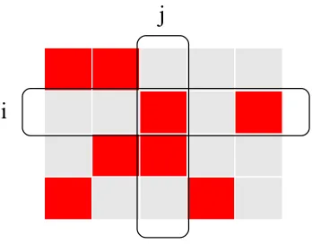
a new ground setZ =L × V of size N =|L| × |V|. Each element of Z corresponds to the index (i, j) of an entry in the assignment matrix A, and selecting elementz= (i, j) means assigning productito userj(see Figure 1 for an illustration). We also denoteZ∗j =L×{j}
and Zi∗ ={i} × V as thej-th column and i-th row of matrix A, respectively. Then, under the above mentioned additional requirements, we would like to find a set of assignments S ⊆ Z so as to maximize the followingoverall influence
f(S) =X
i∈L
aiσi(Ri, Ti), (18)
where σi(Ri, Ti) denote the influence of product ifor a given time Ti,{ai >0} is a set of
weights reflecting the different benefits of the products and Ri ={j ∈ V : (i, j) ∈S}. We
now show that the overall influence functionf(S) in Equation (18) is submodular over the ground setZ.
Lemma 2 Under the continuous-time independent cascade model, the overall influence
i
j
Figure 1: Illustration of the assignment matrix A associated with partition matroid M1 and group knapsack constraints. If product i is assigned to userj, then Aij = 1 (colored
in red). The ground set Z is the set of indices of the entries in A, and selecting an element (i, j)∈ Z means assigning productito userj. The user constraint means that there are at mostuj elements selected in thej-th column; the product constraint means that the total
cost of the elements selected in the i-th row is at most Bi.
Proof By definition, f(∅) = 0 andf(S) is monotone. By Theorem 4 in Gomez-Rodriguez and Sch¨olkopf (2012), the component influence functionσi(Ri, Ti) for productiis
submodu-lar inRi ⊆ V. Since non-negative linear combinations of submodular functions are still sub-modular,fi(S) :=aiσi(Ri, Ti) is also submodular inS⊆ Z =L×V, andf(S) =Pi∈Lfi(S)
is submodular.
3.2 User Constraints
Each social network user can be a potential source and would like to be exposed only to a small number of ads. Furthermore, users may be grouped according to their geographical locations, and advertisers may have a target population they want to reach. Here, we will incorporate these constraints using the matroids which are combinatorial structures that generalize the notion of linear independence in matrices (Schrijver, 2003; Fujishige, 2005). Formulating our constrained influence maximization task with matroids allows us to design a greedy algorithm with provable guarantees.
Formally, suppose that each user j can be assigned to at most uj products. A matroid
can be defined as follows:
Definition 3 A matroid is a pair, M= (Z,I), defined over a finite set (the ground set)
Z and a family of sets (the independent sets) I, that satisfies three axioms:
1. Non-emptiness: The empty set ∅ ∈ I.
2. Heredity: If Y ∈ I and X⊆Y, then X∈ I.
3. Exchange: If X ∈ I, Y ∈ I and |Y| > |X|, then there exists z ∈ Y \X such that
An important type of matroid is the partition matroid where the ground set Z is par-titioned into disjoint subsetsZ1,Z2, . . . ,Zt for somet and
I ={S |S⊆ Z and |S∩ Zi| ≤ui,∀i= 1, . . . , t}
for some given parameters u1, . . . , ut. The user constraints can then be formulated as
Partition matroid M1: partition the ground set Z into Z∗j =L × {j} each of
which corresponds to a column ofA. Then M1={Z,I1} is I1 ={S|S ⊆ Z and |S∩ Z∗j| ≤uj,∀j}.
3.3 Product Constraints
Seeking initial adopters entails a cost to the advertiser, which needs to be paid to the host, while the advertisers of each product have a limited amount of money. Here, we will incorporate these requirements using knapsack constraints which we describe below.
Formally, suppose that each product ihas a budget Bi, and assigning item i to userj
costs cij > 0. Next, we introduce the following notation to describe product constraints
over the ground setZ. For an elementz= (i, j)∈ Z, define its cost asc(z) :=cij. Abusing
the notation slightly, we denote the cost of a subset S⊆ Z asc(S) :=P
z∈Sc(z). Then, in
a feasible solution S ⊆ Z, the cost of assigning producti,c(S∩ Zi∗), should not be larger than its budget Bi.
Now, without loss of generality, we can assume Bi = 1 (by normalizing cij with Bi),
and also cij ∈(0,1] (by throwing away any element (i, j) withcij >1), and define
Group-knapsack: partition the ground set into Zi∗ = {i} × V each of which corresponds to one row of A. Then a feasible solution S⊆ Z satisfies
c(S∩ Zi∗)≤1,∀i.
Importantly, these knapsack constraints have very specific structure: they are on differ-ent groups of a partition {Zi∗} of the ground set and the submodular function f(S) = P
iaiσi(Ri, Ti) is defined over the partition. In consequence, such structures allow us to
design an efficient algorithm with improved guarantees over the known results.
3.4 Overall Problem Formulation
Based on the above discussion of various constraints in viral marketing and our design choices for tackling them, we can think of the influence maximization problem as a special case of the following constrained submodular maximization problem with P = 1 matroid constraints andk=|L| knapsack constraints,
maxS⊆Z f(S) (19)
subject to c(S∩ Zi∗)≤1, 1≤i≤k,
S∈
P
\
p=1 Ip,
Uniform User-Cost. An important case of influence maximization, which we denote as the Uniform Cost, is that for each producti, all users have the same costci∗,i.e.,cij =ci∗. Equivalently, each product i can be assigned to at most bi := bBi/ci∗c users. Then the product constraints are simplified to
Partition matroidM2: for the product constraints with uniform cost, define a matroid M2 ={Z,I2} where
I2 ={S|S⊆ Z and |S∩ Zi∗| ≤bi,∀i}.
In this case, the influence maximization problem defined by Equation (19) becomes the problem withP = 2 matroid constraints and no knapsack constraints (k= 0). In addition, if we assume only one product needs campaign, the formulation of Equation (19) further reduces to the classic influence maximization problem with the simple cardinality constraint.
User Group Constraint. Our formulation in Equation (19) essentially allows for gen-eral matroids which can model more sophisticated real-world constraints, and the proposed formulation, algorithms, and analysis can still hold. For instance, suppose there is a hier-archical community structure on the users, i.e., a tree T where leaves are the users and the internal nodes are communities consisting of all users underneath, such as customers in different countries around the world. In consequence of marketing strategies, on each communityC∈ T, there are at mostuC slots for assigning the products. Such constraints
are readily modeled by the Laminar Matroid, which generalizes the partition matroid by allowing the set {Zi} to be a laminar family (i.e., for any Zi 6= Zj, either Zi ⊆ Zj, or Zj ⊆ Zi, orZi∩ Zj =∅). It can be shown that the community constraints can be captured
by the matroid M= (Z,I) where I ={S⊆ Z :|S∩C| ≤uC,∀C ∈ T }. In the next
sec-tion, we first present our algorithm, then provide the analysis for the uniform cost case and finally leverage such analysis for the general case.
4. Influence Maximization
In this section, we first develop a simple, practical and intuitive adaptive-thresholding greedy algorithm to solve the continuous-time influence maximization problem with the aforemen-tioned constraints. Then, we provide a detailed theoretical analysis of its performance.
4.1 Overall Algorithm
Algorithm 1:Density Threshold Enumeration
Input: parameterδ; objectivef or its approximationfb; assignment costc(z), z∈ Z
1 Set d= max{f({z}) :z∈ Z}; 2 for ρ∈
n 2d
P+2k+1,(1 +δ) 2d
P+2k+1, . . . , 2|Z|d P+2k+1
o do
3 Call Algorithm 2 to getSρ;
Output: argmaxSρf(Sρ)
this is not good enough yet, since in our problem k =|L| can be large, though P = 1 is small.
Here, we will design an algorithm that achieves a better approximation factor by ex-ploiting the following key observation about the structure of the problem defined by Equa-tion (19): the knapsack constraints are over different groups Zi∗ of the whole ground set, and the objective function is a sum of submodular functions over these different groups.
The details of the algorithm, called BudgetMax, are described in Algorithm 1. Bud-getMax enumerates different values of a so-called density thresholdρ, runs a subroutine
to find a solution for each ρ, which quantifies the cost-effectiveness of assigning a particu-lar product to a specific user, and finally outputs the solution with the maximum objective value. Intuitively, the algorithm restricts the search space to be the set of most cost-effective allocations. The details of the subroutine to find a solution for a fixed density threshold ρ are described in Algorithm 2. Inspired by the lazy evaluation heuristic (Leskovec et al., 2007), the algorithm maintains a working set G and a marginal gain threshold wt, which
geometrically decreases by a factor of 1 +δ until it is sufficiently small to be set to zero. At each wt, the subroutine selects each new elementz that satisfies the following properties:
1. It is feasible and the density ratio (the ratio between the marginal gain and the cost) is above the current density threshold;
2. Its marginal gain
f(z|G) :=f(G∪ {z})−f(G)
is above the current marginal gain threshold.
The term “density” comes from the knapsack problem, where the marginal gain is the mass and the cost is the volume. A large density means gaining a lot without paying much. In short, the algorithm considers only high-quality assignments and repeatedly selects feasible ones with marginal gain ranging from large to small.
Algorithm 2:Adaptive Threshold Greedy for Fixed Density
Input: parametersρ,δ; objectivef or its approximationfb; assignment cost
c(z), z∈ Z;set of feasible solutions F; and dfrom Algorithm 1.
1 Set dρ= max{f({z}) :z∈ Z, f({z})≥c(z)ρ}; 2 Set wt= (1+dρδ)t fort= 0, . . . , L= argmini
wi≤ δdN
and wL+1 = 0;
3 Set G=∅;
4 for t= 0,1, . . . , L, L+ 1do
5 forz6∈G with G∪ {z} ∈ F and f(z|G)≥c(z)ρ do 6 if f(z|G)≥wtthen
7 SetG←G∪ {z};
Output: Sρ=G
Remark 2. Evaluating the influence of the assigned productsf is expensive. Therefore, we will use the randomized algorithm in Section 2.4.3 to compute an estimationfb(·) of the quantityf(·).
4.2 Theoretical Guarantees
Although our algorithm is quite intuitive, it is highly non-trivial to obtain the theoretical guarantees. For clarity, we first analyze the simpler case with uniform cost, which then provides the base for analyzing the general case.
4.2.1 Uniform Cost
As shown at the end of Section 3.4, the influence maximization, in this case, corresponds to the problem defined by Equation (19) with P = 2 and no knapsack constraints. Thus, we can simply run Algorithm 2 with ρ = 0 to obtain a solution G, which is roughly a
1
P+1-approximation.
Intuition. The algorithm greedily selects feasible elements with sufficiently large marginal gain. However, it is unclear whether our algorithm will findgood solutions and whether it will berobust to noise. Regarding the former, one might wonder whether the algorithm will select just a few elements while many elements in the optimal solutionOwill become infea-sible and will not be selected, in which case the greedy solutionGis a poor approximation. Regarding the latter, we only use the estimationfbof the influencef (i.e.,|fb(S)−f(S)| ≤ for anyS ⊆ Z), which introduces additional error to the function value. A crucial question, which has not been addressed before (Badanidiyuru and Vondr´ak, 2014), is whether the adaptive threshold greedy algorithm is robust to such perturbations.
G
O\G
g1
C1
gt−1
Ct−1
gt
Ct
g|G|
C|G|
· · · ·
g2
C2 St
i=1Ci
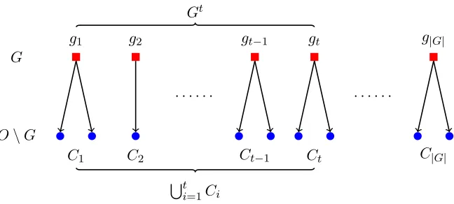
Gt
Figure 2: Notation for analyzing Algorithm 2. The elements in the greedy solution G are arranged according to the order in which Algorithm 2 selects them in Step 3. The elements in the optimal solution O but not in the greedy solution G are partitioned into groups {Ct}1≤t≤|G|, whereCt are those elements in O\G that are still feasible before selecting gt
but are infeasible after selecting gt.
element in the group associated with it (up to some small error). This means that even if the submodular function evaluation is inexact, the quality of the elements in the greedy solution is still good. The two claims together show that the marginal gain of O\Gis not much larger than the gain of G, and thus G is a good approximation for the problem.
Formally, suppose we use an inexact evaluation of the influence f such that |fb(S)−
f(S)| ≤ for any S ⊆ Z, let product i ∈ L spread according to a diffusion network Gi= (V,Ei), and i∗ = argmaxi∈L|Ei|. Then, we have:
Theorem 4 Suppose fbis evaluated up to error =δ/16 with ConTinEst. For influence
maximization with uniform cost, Algorithm 2 (withρ= 0) outputs a solutionGwithf(G)≥
1−2δ
3 f(O) in expected timeOe
|E i∗|+|V|
δ2 +
|L||V| δ3
.
The parameter δ introduces a tradeoff between the approximation guarantee and the runtime: larger δ decreases the approximation ratio but results in fewer influence evalua-tions. Moreover, the runtime has a linear dependence on the network size and the number of products to propagate (ignoring some small logarithmic terms) and, as a consequence, the algorithm is scalable to large networks.
Analysis. SupposeG={g1, . . . , g|G|} in the order of selection, and let Gt={g1, . . . , gt}.
Let Ct denote all those elements in O\Gthat satisfy the following: they are still feasible
before selecting thet-th elementgtbut are infeasible after selectinggt. Equivalently,Ctare
all those elementsj∈O\Gsuch that (1)j∪Gt−1 does not violate the matroid constraints but (2) j∪Gt violates the matroid constraints. In other words, we can think of Ct as the
optimal elements “blocked” bygt. Then, we proceed as follows.
By the property of the intersection of matroids, the size of the prefixSt
{z} ∪T2 violates at least one of the matroid constraints since T2 is maximal. Then, let {Vi}1≤i≤P denote all elements inT1\T2 that violate the i-th matroid, and partitionT1∩T2 arbitrarily among theseVi’s so that they coverT1. In this construction, the size of eachVi
must be at most|T2|, since otherwise by the Exchange axiom, there would existz∈Vi\T2 that can be added to T2, without violating the i-th matroid, leading to a contradiction. Therefore, |T1|is at mostP times|T2|.
Next, we apply the above property as follows. Let Q be the union of Gt and St
i=1Ct.
On one hand, Gt is a maximal independent subset of Q, since no element in St
i=1Ct can be added to Gt without violating the matroid constraints. On the other hand, St
i=1Ct is an independent subset ofQ, since it is part of the optimal solution. Therefore,St
i=1Cthas
size at most P times|Gt|, which is P t. Note that the properties of matroids are crucial for this analysis, which justifies our formulation using matroids. In summary, we have
Claim 1 Pt
i=1|Ci| ≤P t, for t= 1, . . . ,|G|.
Now, we consider the marginal gain of each element in Ct associated with gt. First,
supposegtis selected at the thresholdτt>0. Then, anyj∈Cthas marginal gain bounded
by (1 +δ)τt+ 2, since otherwise j would have been selected at a larger threshold beforeτt
by the greedy criterion. Second, suppose gt is selected at the threshold wL+1 = 0. Then, any j ∈Ct has marginal gain approximately bounded by Nδd. Since the greedy algorithm
must pick g1 with fb(g1) =d and d≤f(g1) +, anyj ∈Ct has marginal gain bounded by
δ
Nf(G) +O(). Putting everything together we have:
Claim 2 Supposegtis selected at the thresholdτt. Thenf(j|Gt−1)≤(1+δ)τt+4+Nδf(G)
for anyj ∈Ct.
Since the evaluation of the marginal gain ofgt should be at leastτt, this claims essentially
indicates that the marginal gain ofj is approximately bounded by that of gt.
Since there are not many elements inCt (Claim 1) and the marginal gain of each of its
elements is not much larger than that of gt (Claim 2), we can conclude that the marginal
gain ofO\G=S|G|
i=1Ctis not much larger than that of G, which is just f(G). Claim 3 The marginal gain ofO\Gsatisfies
X
j∈O\G
f(j|G)≤[(1 +δ)P +δ]f(G) + (6 + 2δ)P|G|.
Finally, since by submodularity, f(O) ≤ f(O∪G) ≤ f(G) +P
j∈O\Gf(j|G), Claim 3
shows thatf(G) is close tof(O) up to a multiplicative factor roughly (1 +P) and additive factor O(P|G|). Given that f(G) >|G|, it leads to roughly a 1/3-approximation for our influence maximization problem by setting=δ/16 when evaluatingfbwithConTinEst. Combining the above analysis and the runtime of the influence estimation algorithm, we have our final guarantee in Theorem 4. Appendix D.1 presents the complete proofs.
4.2.2 General Case
Intuition. The key idea behind Algorithm 1 and Algorithm 2 is simple: spend the budgets
efficiently and spend them as much as possible. By spending them efficiently, we mean to
only select those elements whose density ratio between the marginal gain and the cost is above the threshold ρ. That is, we assign product i to userj only if the assignment leads to large marginal gain without paying too much. By spending the budgets as much as possible, we mean to stop assigning product ionly if its budget is almost exhausted or no more assignments are possible without violating the matroid constraints. Here we make use of the special structure of the knapsack constraints on the budgets: each constraint is only related to the assignment of the corresponding product and its budget, so that when the budget of one product is exhausted, it does not affect the assignment of the other products. In the language of submodular optimization, the knapsack constraints are on a partition Zi∗ of the ground set and the objective function is a sum of submodular functions over the partition.
However, there seems to be a hidden contradiction between spending the budgets effi-ciently and spending them as much as possible. On one hand, efficiency means the density ratio should be large, so the threshold ρ should be large; on the other hand, if ρ is large, there are just a few elements that can be considered, and thus the budget might not be exhausted. After all, if we set ρ to be even larger than the maximum possible value, then no element is considered and no gain is achieved. In the other extreme, if we setρ= 0 and consider all the elements, then a few elements with large costs may be selected, exhausting all the budgets and leading to a poor solution.
Fortunately, there exists a suitable threshold ρ that achieves a good tradeoff between the two and leads to a good approximation. On one hand, the threshold is sufficiently small, so that the optimal elements we abandon (i.e., those with low-density ratio) have a total gain at most a fraction of the optimum; on the other hand, it is also sufficiently large, so that the elements selected are of high quality (i.e., of high-density ratio), and we achieve sufficient gain even if the budgets of some items are exhausted.
Theorem 5 Supposefbis evaluated up to error=δ/16withConTinEst. In Algorithm 1,
there exists a ρ such that
f(Sρ)≥
max{ka,1}
(2|L|+ 2)(1 + 3δ)f(O)
where ka is the number of active knapsack constraints:
ka=|{i:Sρ∪ {z} 6∈ F,∀z∈ Zi∗}|.
The expected running time is Oe
|E i∗|+|V|
δ2 +
|L||V| δ4
.
Importantly, the approximation factor improves over the best known guarantee P+21k+1 = 1
Analysis. The analysis follows the intuition. Pick ρ = P2+2f(kO+1) , where O is the optimal solution, and define
O−:={z∈O\Sρ:f(z|Sρ)< c(z)ρ+ 2}, O+:={z∈O\Sρ:z6∈O−}.
Note that, by submodularity, O− is a superset of the elements in the optimal solution that we abandon due to the density threshold and, by construction, its marginal gain is small:
f(O−|Sρ)≤ρc(O−) +O(|Sρ|)≤kρ+O(|Sρ|),
where the small additive term O(|Sρ|) is due to inexact function evaluations. Next, we
proceed as follows.
First, if no knapsack constraints are active, then the algorithm runs as if there were no knapsack constraints (but only on elements with density ratio aboveρ). Therefore, we can apply the same argument as in the case of uniform cost (refer to the analysis up to Claim 3 in Section 4.2.1); the only caveat is that we apply the argument to O+ instead of O\Sρ.
Formally, similar to Claim 3, the marginal gain of O+ satisfies
f(O+|Sρ)≤[(1 +δ)P+δ]f(Sρ) +O(P|Sρ|),
where the small additive term O(P|Sρ|) is due to inexact function evaluations. Using
that f(O)≤f(Sρ) +f(O−|Sρ) +f(O+|Sρ), we can conclude that Sρis roughly a P+21k+1
-approximation.
Second, supposeka>0 knapsack constraints are active and the algorithm discovers that
the budget of productiis exhausted when trying to add elementzto the setGi=G∩Zi∗ of selected elements at that time. Sincec(Gi∪ {z})>1 and each of these elements has density
aboveρ, the gain ofGi∪ {z} is aboveρ. However, only Gi is included in our final solution,
so we need to show that the marginal gain of z is not large compared to that ofGi. To do
so, we first realize that the algorithm greedily selects elements with marginal gain above a decreasing threshold wt. Then, since z is the last element selected and Gi is nonempty
(otherwise adding zwill not exhaust the budget), the marginal gain ofz must be bounded by roughly that ofGi, which is at least roughly 12ρ. Since this holds for all active knapsack
constraints, then the solution has value at least ka
2 ρ, which is an
ka
P+2k+1-approximation. Finally, combining both cases, and setting k = |L| and P = 1 as in our problem, we have our final guarantee in Theorem 5. Appendix D.2 presents the complete proofs.
5. Experiments on Synthetic and Real Data
In this section, we first evaluate the accuracy of the estimated influence given by Con-TinEst and then investigate the performance of influence maximization on synthetic and
real networks by incorporatingConTinEstinto the framework of BudgetMax. We show
Core-p
erphery
T
2 4 6 8 10
Influence 0 50 100 150 200 NS ConTinEst
102 103 104
0 0.02 0.04 0.06 0.08 #samples relative error
5 10 20 30 40 50
0 2 4 6 8
x 10−3
#labels
relative error
Random
T
2 4 6 8 10
Influence 0 5 10 15 20 NS ConTinEst
102 103 104
0 0.02 0.04 0.06 0.08 #samples relative error
10 20 30 40 50
0 2 4 6 8
x 10−3
#labels relative error Hierarc h y T
2 4 6 8 10
Influence 1 2 3 4 5 6 7 8 9 NS ConTinEst
102 103 104
0 0.02 0.04 0.06 0.08 #samples relative error
10 20 30 40 50
0 2 4 6 8
x 10−3
#labels
relative error
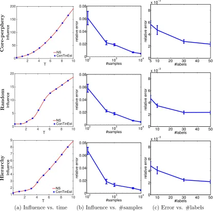
(a) Influence vs. time (b) Influence vs. #samples (c) Error vs. #labels
Figure 3: Influence estimation for core-periphery, random, and hierarchical networks with 1,024 nodes and 2,048 edges. Column (a) shows estimated influence by NS (near ground truth), and ConTinEst for increasing time window T; Column (b) shows ConTinEst’s
relative error against number of samples with 5 random labels and T = 10; Column (c) re-portsConTinEst’s relative error against the number of random labels with 10,000 random
5.1 Experiments on Synthetic Data
We generate three types of Kronecker networks (Leskovec et al., 2010) which are synthetic networks generated by a recursive Kronecker product of a base 2-by-2 parameter matrix with itself to generate self-similar graphs. By tuning the base parameter matrix, we are able to generate the Kronecker networks which can mimic different structural properties of many real networks. In the following, we consider networks of three different types of structures: (i) core-periphery networks (parameter matrix: [0.9 0.5; 0.5 0.3]), which mimic the information diffusion traces in real-world networks (Gomez-Rodriguez et al., 2011), (ii) random networks ([0.5 0.5; 0.5 0.5]), typically used in physics and graph theory (Easley and Kleinberg, 2010) and (iii) hierarchical networks ([0.9 0.1; 0.1 0.9]) (Clauset et al., 2008). Next, we assign a pairwise transmission function for every directed edge in each type of network and set its parameters at random. In our experiments, we use the Weibull distribution from (Aalen et al., 2008),
f(t;α, β) = β α
t α
β−1
e−(t/α)β, t≥0, (20)
whereα >0 is a scale parameter andβ >0 is a shape parameter. The Weibull distribution (Wbl) has often been used to model lifetime events in survival analysis, providing more flexibility than an exponential distribution. We choose α and β from 0 to 10 uniformly at random for each edge in order to have heterogeneous temporal dynamics. Finally, for each type of Kronecker network, we generate 10 sample networks, each of which has differentα and β chosen for every edge.
5.1.1 Influence Estimation
To the best of our knowledge, there is no analytical solution to the influence estimation given Weibull transmission function. Therefore, we compare ConTinEst with the Naive
Sampling (NS) approach by considering the highest degree node in a network as the source, and draw 1,000,000 samples for NS to obtain near ground truth. In Figure 3, Column (a) compares ConTinEst with the ground truth provided by NS at different time window T, from 0.1 to 10 in networks of different structures. For ConTinEst, we generate up
to 10,000 random samples (or sets of random waiting times), and 5 random labels in the inner loop. In all three networks, estimation provided byConTinEstfits the ground truth
accurately, and the relative error decreases quickly as we increase the number of samples and labels (Column (b) and Column (c)). For 10,000 random samples with 5 random labels, the relative error is smaller than 0.01.
5.1.2 Influence Maximization with Uniform Cost
In this section, we first evaluate the effectiveness of ConTinEst to the classic influence
Influence
b
y
Size
0 10 20 30 40 50
#sources 0 50 100 150 200 250 300 350 400 450 influence ConTinEst(Wbl) ConTinEst(Exp) Greedy(IC) SP1M PMIA MIA-M
0 10 20 30 40 50
#sources 0 50 100 150 200 250 300 350 400 influence ConTinEst(Wbl) ConTinEst(Exp) Greedy(IC) SP1M PMIA MIA-M
0 10 20 30 40 50
#sources 0 50 100 150 200 250 300 influence ConTinEst(Wbl) ConTinEst(Exp) Greedy(IC) SP1M PMIA MIA-M Influence b y Time
0 1 2 3 4 5
T 0 50 100 150 200 250 300 350 400 450 influence ConTinEst(Wbl) ConTinEst(Exp) Greedy(IC) SP1M PMIA MIA-M
0 1 2 3 4 5
T 0 50 100 150 200 250 300 350 400 influence ConTinEst(Wbl) ConTinEst(Exp) Greedy(IC) SP1M PMIA MIA-M
0 1 2 3 4 5
T 0 50 100 150 200 250 300 influence ConTinEst(Wbl) ConTinEst(Exp) Greedy(IC) SP1M PMIA MIA-M
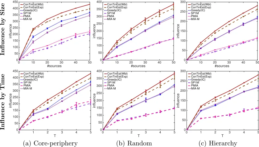
(a) Core-periphery (b) Random (c) Hierarchy
Figure 4: Influence σ(A, T) achieved by varying number of sources |A| and observation window T on the networks of different structures with 1,024 nodes, 2,048 edges and het-erogeneous Weibull transmission functions. Top row: influence against #sources by T = 5; Bottom row: influence against the time windowT using 50 sources.
4 8 16 32 64
0 0.5 1 1.5
2x 10 4 # products influence Uniform Cost BudgetMax GreedyDegree Random
4 8 12 16 20
0 0.5 1 1.5 2 2.5
3x 10
4 product constraints influence Uniform Cost BudgetMax GreedyDegree Random
2 4 6 8 10
0 0.5 1 1.5 2 2.5x 10
4 user constraints influence Uniform Cost BudgetMax GreedyDegree Random
(a) By products (b) By product constraints (c) By user constraints
Figure 5: Over the 64 product-specific diffusion networks, each of which has 1,048,576 nodes, the estimated influence (a) for increasing the number of products by fixing the product-constraint at 8 and user-constraint at 2; (b) for increasing product-constraint by user-constraint at 2; and (c) for increasing user-constraint by fixing product-constraint at 8. For all experiments, we have T = 5 time window.
we fit an exponential distribution per edge by NetRate (Gomez-Rodriguez et al., 2011).
Furthermore,Influmaxis not scalable. When the average network density (defined as the
is more than 24 hours. In consequence, we present the results of ConTinEst using fitted
exponential distributions (Exp). For the discrete-time IC model, we learn the infection probability within time window T using Netrapalli’s method (Netrapalli and Sanghavi, 2012). The learned pairwise infection probabilities are also served for SP1M and PMIA,
which approximately calculate the influence based on the IC model. For the discrete-time LT model, we set the weight of each incoming edge to a node u to the inverse of its in-degree, as in previous work (Kempe et al., 2003), and choose each node’s threshold uniformly at random. The top row of Figure 4 compares the expected number of infected nodes against the source set size for different methods. ConTinEst outperforms the rest,
and the competitive advantage becomes more dramatic the larger the source set grows. The bottom row of Figure 4 shows the expected number of infected nodes against the time window for 50 selected sources. Again, ConTinEst performs the best for all three types
of networks.
Next, usingConTinEstas a subroutine for influence estimation, we evaluate the
perfor-mance of BudgetMaxwith the uniform-cost constraints on the users. In our experiments
we consider up to 64 products, each of which diffuses over one of the above three different types of Kronecker networks with∼one million nodes. Further, we randomly select a subset of 512 nodes VS ⊆ V as our candidate target users, who will receive the given products, and evaluate the potential influence of an allocation over the underlying one-million-node networks. ForBudgetMax, we set the adaptive threshold δ to 0.01 and the cost per user
and product to 1. For ConTinEst, we use 2,048 samples with 5 random labels on each
of the product-specific diffusion networks. We repeat our experiments 10 times and report the average performance.
We compare BudgetMax with a nodes’ degree-based heuristic, which we refer to as
GreedyDegree, where the degree is treated as a natural measure of influence, and a baseline method, which assigns the products to the target nodes randomly. We opt for the nodes’ degree-based heuristic since, in practice, large-degree nodes, such as users with millions of followers in Twitter, are often the targeted users who will receive a considerable payment if he (she) agrees to post the adoption of some products (or ads) from merchants. GreedyDe-gree proceeds as follows. It first sorts the list of all pairs of productsiand nodesj∈ VS in
descending order of node-j’s degree in the diffusion network associated to producti. Then, starting from the beginning of the list, it considers each pair one by one: if the addition of the current pair to the existing solution does not violate the predefined matroid constraints, it is added to the solution, and otherwise, it is skipped. This process continues until the end of the list is reached. In other words, we greedily assign products to nodes with the largest degree. Due to the large size of the underlying diffusion networks, we do not apply other more expensive node centrality measures such as the clustering coefficient and betweenness. Figure 5 summarizes the results. Panel (a) shows the achieved influence against number of products, fixing the budget per product to 8 and the budget per user to 2. As the number of products increases, on the one hand, more and more nodes become assigned, so the total influence will increase. Yet, on the other hand, the competition among products for a few existinginfluential nodes also increases. GreedyDegree achieves a modest performance, since high degree nodes may have many overlapping children. In contrast,BudgetMax, by
of product (i.e., the competition) increases. Panel (b) shows the achieved influence against the budget per product, considering 64 products and fixing the budget per user to 2. We find that, as the budget per product increases, the performance of GreedyDegree tends to flatten and the competitive advantage of BudgetMax becomes more dramatic. Finally,
Panel (c) shows the achieved influence against the budget per user, considering 64 products and fixing the budget per product to 8. We find that, as the budget per user increases, the influence only increases slowly. This is due to the fixed budget per product, which prevents additional new nodes to be assigned. This meets our intuition: by making a fixed number of people watching more ads per day, we can hardly boost the popularity of the product. Additionally, even though the same node can be assigned to more products, there is hardly ever a node that is the perfect source from which all products can efficiently spread.
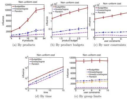
5.1.3 Influence Maximization with Non-Uniform Cost
In this section, we evaluate the performance of BudgetMax under non-uniform cost
con-straints, using againConTinEstas a subroutine for influence estimation. Our designing of
user-cost aim to mimic a real scenario, where advertisers pay much more money to celebri-ties with millions of social network followers than to normal citizens. To do so, we let ci ∝d1i/n where ci is the cost, di is the degree, and n≥1 controls the increasing speed of
cost with respect to the degree. In our experiments, we use n= 3 and normalize ci to be
within (0,1]. Moreover, we set the product-budget to a base value from 1 to 10 and add a random adjustment drawn from a uniform distributionU(0,1).
We compare our method to two modified versions of the above mentioned nodes’ degree-based heuristic GreedyDegree and to the same baseline method. In the first modified version of the heuristic, which we still refer to as GreedyDegree, takes both the degree and the corresponding cost into consideration. In particular, it sorts the list of all pairs of products iand nodes j∈ VS in descending order of degree-cost ratio dj/cj in the diffusion
network associated to product i, instead of simply the node-j’s degree, and then proceeds similarly as before. In the second modified version of the heuristic, which we refer as GreedyLocalDegree, we use the same degree-cost ratio but allow the target users to be partitioned into distinct groups (or communities) and pick the most cost-effective pairs within each group locally instead. Figure 6 compares the performance of our method with the competing methods against four factors: (a) the number of products, (b) the budget per product, (c) the budget per user and (d) the time window T, while fixing the other factors. In all cases, BudgetMax significantly outperforms the other methods, and the
achieved influence increases monotonically with respect to the factor value, as one may have expected. In addition, in Figure 6(e), we study the effect of the Laminar matroid combined with group knapsack constraints, which is the most general type of constraint we handle in this paper (refer to Section 3.4). The selected target users are further partitioned into K groups randomly, each of which has, Qi, i = 1. . . K, limit which constrains the maximum
allocations allowed in each group. In practical scenarios, each group might correspond to a geographical community or organization. In our experiment, we divide the users into 8 equal-size groups and setQi = 16, i= 1. . . Kto indicate that we want a balanced allocation
4 8 16 32 64 0
2000 4000 6000 8000 10000 12000
# products
influence
Non−uniform cost
BudgetMax GreedyDegree Random
1 1.5 2 2.5 3 0
0.5 1 1.5
2x 10 4
product budget
influence
Non−uniform cost
BudgetMax GreedyDegree Random
2 4 6 8 10
0 0.5 1 1.5
2x 10
4
user constraints
influence
Non−uniform cost
BudgetMax GreedyDegree Random
(a) By products (b) By product budgets (c) By user constraints
2 5 10 15
102 104 106 108
time
influence
Non−uniform cost
BudgetMax GreedyDegree Random
2 4 6 8 10
0 2000 4000 6000 8000 10000 12000
user constraints
influence
Non−uniform cost
BudgetMax GreedyDegree GreedyLocalDegree Random
(d) By time (e) By group limits
1 5 10 15 20 25 30 35 40 45 50 0
0.2 0.4 0.6 0.8 1
δ
accuracy
Uniform cost
BudgetMax(Adaptive) BudgetMax(Lazy)
1 5 10 15 20 25 30 35 40 45 50 0
10 20 30 40 50 60 70
δ
time(s)
Uniform cost
BudgetMax(Adaptive) BudgetMax(Lazy)
(a) δ vs. accuracy (b)δ vs. time
Figure 7: The relative accuracy and the run-time for different threshold parameter δ.
estimated influence does not increase significantly with respect to the budget (i.e., number of slots) per user. This is due to the fixed budget per group, which prevents additional new nodes to be assigned, even though the number of available slots per user increases.
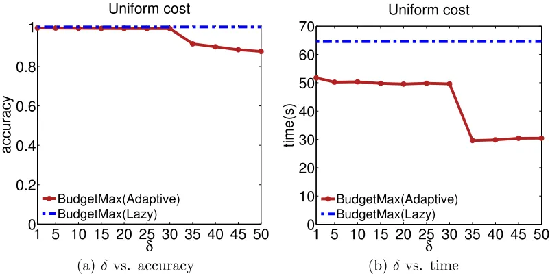
5.1.4 Effects of Adaptive Thresholding
In Figure 7, we investigate the impact that the threshold value δ has on the accuracy and runtime of our adaptive thresholding algorithm and compare it with the lazy evaluation method. Note that the performance and runtime of lazy evaluation do not change with respect toδbecause it does not depend on it. Panel (a) shows the achieved influence against the thresholdδ. As expected, the larger the δ value, the lower the accuracy. However, our method is relatively robust to the particular choice ofδsince its performance is always over a 90-percent relative accuracy even for large δ. Panel (b) shows the runtime against the threshold δ. In this case, the larger the δ value, the lower the runtime. In other words, Figure 7 verifies the intuition thatδ is able to trade off the solution quality of the allocation with the runtime time.
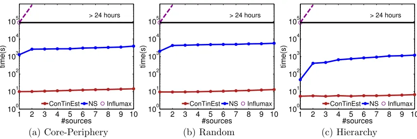
5.1.5 Scalability
In this section, we start with evaluating the scalability of the proposed algorithms on the classic influence maximization problem where we only have one product with the cardinality constraint on the users.
We compare it to the state-of-the-art methodInflumax(Gomez-Rodriguez and Sch¨olkopf,
2012) and the Naive Sampling (NS) method in terms of runtime for the continuous-time influence estimation and maximization. For ConTinEst, we draw 10,000 samples in the
outer loop, each having 5 random labels in the inner loop. We plugConTinEst as a
1 2 3 4 5 6 7 8 9 10 100 101 102 103 104 105 #sources time(s)
ConTinEst NS Influmax > 24 hours
1 2 3 4 5 6 7 8 9 10
100 101 102 103 104 105 #sources time(s)
ConTinEst NS Influmax > 24 hours
1 2 3 4 5 6 7 8 9 10
100 101 102 103 104 105 #sources time(s)
ConTinEst NS Influmax > 24 hours
(a) Core-Periphery (b) Random (c) Hierarchy
Figure 8: Runtime of selecting increasing number of sources on Kronecker networks of 128 nodes and 320 edges with T = 10.
1.5 2 2.5 3 3.5 4 4.5 5
100 101 102 103 104 105 density time(s)
ConTinEst NS Influmax > 24 hours
1.5 2 2.5 3 3.5 4 4.5 5
100 101 102 103 104 105 density time(s)
ConTinEst NS Influmax > 24 hours
1.5 2 2.5 3 3.5 4 4.5 5
100 101 102 103 104 105 density time(s)
ConTinEst NS Influmax > 24 hours
(a) Core-Periphery (b) Random (c) Hierarchy
Figure 9: Runtime of selecting 10 sources in networks of 128 nodes with increasing density by T = 10.
Figure 8 compares the performance of increasingly selecting sources (from 1 to 10) on small Kronecker networks. When the number of selected sources is 1, different algorithms essentially spend time estimating the influence for each node. ConTinEst outperforms
other methods by order of magnitude and for the number of sources larger than 1, it can efficiently reuse computations for estimating influence for individual nodes. Dashed lines mean that a method did not finish in 24 hours, and the estimated run time is plotted.
Next, we compare the run time for selecting 10 sources with increasing densities (or the number of edges) in Figure 9. Again,Influmaxand NS are order of magnitude slower due
to their respective exponential and quadratic computational complexity in network density. In contrast, the run time of ConTinEstonly increases slightly with the increasing density
since its computational complexity is linear in the number of edges. We evaluate the speed on large core-periphery networks, ranging from 100 to 1,000,000 nodes with density 1.5 in Figure 10. We report the parallel run time only for ConTinEst and NS (both are
implemented by MPI running on 192 cores of 2.4Ghz) since Influmax is not scalable. In
contrast to NS, the performance of ConTinEst increases linearly with the network size
102 103 104 105 106 102
103 104 105 106
#nodes
time(s)
ConTinEst NS > 48 hours
Figure 10: For core-periphery networks by T = 10, runtime of selecting 10 sources with increasing network size from 100 to 1,000,000 by fixing 1.5 network density.
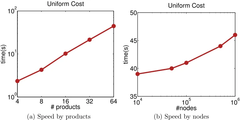
4 8 16 32 64
100 101 102
time(s)
# products Uniform Cost
104 105 106
35 40 45 50
time(s)
#nodes Uniform Cost
(a) Speed by products (b) Speed by nodes