The Thirty-Third AAAI Conference on Artificial Intelligence (AAAI-19)
ACE: An Actor Ensemble Algorithm for Continuous Control with Tree Search
Shangtong Zhang,
∗1Hengshuai Yao
2 1Department of Computing Science, University of Alberta2Reinforcement Learning for Autonomous Driving Lab, Noah’s Ark Lab, Huawei [email protected], [email protected]
Abstract
In this paper, we propose an actor ensemble algorithm, named ACE, for continuous control with a deterministic policy in re-inforcement learning. In ACE, we use actor ensemble (i.e., multiple actors) to search the global maxima of the critic. Besides the ensemble perspective, we also formulate ACE in the option framework by extending the option-critic ar-chitecture with deterministic intra-option policies, revealing a relationship between ensemble and options. Furthermore, we perform a look-ahead tree search with those actors and a learned value prediction model, resulting in a refined value estimation. We demonstrate a significant performance boost of ACE over DDPG and its variants in challenging physical robot simulators.
Introduction
In this paper, we propose an actor ensemble algorithm, named ACE, for continuous control in reinforcement learn-ing (RL). In continuous control, a deterministic policy (Sil-ver et al. 2014) is a recent approach, which is a mapping from state to action. In contrast, a stochastic policy is a map-ping from state to a probability distribution over the actions. Recently, neural networks has achieved great success as function approximators in various challenging domains (Tesauro 1995; Mnih et al. 2015; Silver et al. 2016). A deter-ministic policy parameterized by a neural network is usually trained via gradient ascent to maximize the critic, which is a state-action value function parameterized by a neural net-work (Silver et al. 2014; Lillicrap et al. 2015; Barth-Maron et al. 2018). However, gradient ascent can be easily trapped by local maxima during the search for the global maxima. We utilize the ensemble technique to mitigate this issue. We train multiple actors (i.e., deterministic policies) in parallel, and each actor has a different initialization. In this way, each actor is in charge of maximizing the state-action value func-tion in a local area. Different actors may be trapped in differ-ent local maxima. By considering the maximum state-action value of the actions proposed by all the actors, we are more likely to find the global maxima of the state-action value function than a single actor.
∗
Work done during an internship at Huawei
Copyright c2019, Association for the Advancement of Artificial Intelligence (www.aaai.org). All rights reserved.
ACE fits in with the option framework (Sutton, Precup, and Singh 1999). First, each option has its intra-option pol-icy, which maximizes the return in a certain area of the state space. Similarly, an actor in ACE maximizes the critic in a certain area of the domain of the critic. It may be difficult for a single actor to maximize the critic in the whole domain due to the complexity of the manifold of the critic. However, in contrast, the job for action search is easier if we ask an actor to find the best action in a local neighborhood of the action dimension. Second, we chain the outputs of all the actors to the critic, enabling a selection over the locally optimal action values. In this way, the critic works similar to the policy over options in the option framework. We quantify this similarity between ensemble and options by extending the option-critic architecture (OCA, Bacon, Harb, and Precup 2017) with de-terministic intra-option policies. Particularly, we provide the Deterministic Intra-option Policy Gradient theorem, based on which we show the actor ensemble in ACE is a special case of the general option-critic framework.
To make the state-action value function more accurate, which is essential in the actor selection, we perform a look-ahead tree search with the multiple actors. The look-look-ahead tree search has achieved great success in various discrete ac-tion problems (Knuth and Moore 1975; Browne et al. 2012; Silver et al. 2016; Oh, Singh, and Lee 2017; Farquhar et al. 2018). Recently, look-ahead tree search was extended to continuous-action problems. For example, Mansley, We-instein, and Littman (2011) combined planning with adap-tive discretization of a continuous action space, resulting in a performance boost in continuous bandit problems. Nitti, Belle, and De Raedt (2015) utilized probability program-ming in planning in continuous action space. Yee, Lis`y, and Bowling (2016) used kernel regression to generalize the val-ues between explored actions and unexplored actions, result-ing in a new Monte Carlo tree search algorithm. However, to our best knowledge, a general tree search algorithm for continuous-action problems is a gap. In ACE, we use the multiple actors as meta-actions to perform a tree search with the help of a learned value prediction model (Oh, Singh, and Lee 2017; Farquhar et al. 2018).
We demonstrate the superiority of ACE over DDPG and its variants empirically in Roboschool1, a challenging
phys-1
ical robot environment.
In the rest of this paper, we first present some preliminar-ies of RL. Then we detail ACE and show some empirical results, after which we discuss some related work, followed by closing remarks.
Preliminaries
We consider a Markov Decision Process (MDP) which con-sists of a state spaceS, an action spaceA, a reward function
r:S × A →R, a transition kernelp:S × A × S →[0,1],
and a discount factorγ∈[0,1]. We useπ:S × A →[0,1]
to denote a stochastic policy. At each time stept, an agent is at statestand selects an action at ∼ π(·|st). Then the environment gives the reward rt+1 and leads the agent to
the next state st+1 accordingp(·|st, at). We useqπ to de-note the state action value of a policy π, i.e., qπ(s, a) =.
Eπ[P∞t=0γtrt+1|s0 = s, a0 = a]. In an RL problem, we
are usually interested in finding an optimal policy π∗ s.t.
qπ∗(s, a)≥qπ(s, a)for∀(π, s, a). All the optimal policies share the same optimal state action value functionq∗, which is the unique fixed point of the Bellman optimality operator T,
TQ(s, a)=. r(s, a) +γEs0∼p(·|s,a)[max
a0 Q(s
0, a0)] (1)
where we useQto indicate an estimation ofq∗. With tabular representation, Q-learning (Watkins and Dayan 1992) is a commonly used method to find this fixed point. The per step update is
∆Q(st, at)∝rt+1+γmax
a Q(st+1, a)−Q(st, at) (2) Recently, Mnih et al. (2015) used a deep convolutional neural networkθ to parameterize an estimationQ, result-ing in the Deep-Q-Network (DQN). At each time step t, DQN samples the transition(st, at, rt+1, st+1)from a
re-play buffer (Lin 1992) and performs stochastic gradient de-scent to minimize the loss
1
2 rt+1+γmaxa Qθ
−(st+1, a)−Qθ(st, at)
2
whereθ−is a target network (Mnih et al. 2015), which is a copy ofθand is synchronized withθperiodically.
Continuous Action Control
In continuous control problems, it is not straightforward to apply Q-learning. The basic idea of the deterministic pol-icy algorithms (Silver et al. 2014) is to use a determinis-tic policy µ : S → A to approximate the greedy action
arg maxaQ(s, a). The deterministic policy is trained via gradient ascent according to chain rule. The gradient per step is
∇θµQ(st, µ(st)) =∇aQ(s, a)|s=s
t,a=µ(st)∇θµµ(s)|s=st
(3)
where we assumeµis parameterized byθµ. With this actor
µ, we are able to update the state action value functionQas usual. To be more specific, assumingQis parameterized by
θQ, we perform gradient decent to minimize the following loss
1
2 rt+1+γQ(st+1, µ(st+1))−Q(st, at)
2
Recently, Lillicrap et al. (2015) used neural networks to pa-rameterizeµandQ, resulting in the Deep Deterministic Pol-icy Gradient (DDPG) algorithm. DDPG is an off-polPol-icy con-trol algorithm with experience replay and a target network.
In the on-policy setting, the gradient in Equation (3) guar-antees policy improvement thanks to the Deterministic Pol-icy Gradient theorem (Silver et al. 2014). In off-polPol-icy set-ting, the policy improvement of this gradient is based on Off-policy Policy Gradient theorem (OPG, Degris, White, and Sutton 2012). However, Errata of Degris, White, and Sutton (2012) shows that OPG only holds for tabular function rep-resentation and certain linear function approximation. So far no policy improvement is guaranteed for DDPG. However, DDPG and its variants has gained great success in various challenging domains (Lillicrap et al. 2015; Barth-Maron et al. 2018; Tassa et al. 2018). This success may be attributed to the gradient ascent via chain rule in Equation (3).
Option
An optionω is a triple,(Iω, πω, βω), and we use Ωto in-dicate the option set. We use Iω ⊆ S to denote the ini-tiation set of ω, indicating where the option ω can be ini-tiated. In this paper, we consider Iω ≡ S for ∀ω, mean-ing that each option can be initiated at all states. We use
πω:S × A →[0,1]to denote the intra-option policy ofω. Once the optionωis committed, the action selection is based onπω. We use βω : S → [0,1]to denote the termination function ofω. At each time stept, the agent terminates the previous optionωt−1with probabilityβωt−1(st). In this
pa-per, we consider thecall-and-returnoption execution model (Sutton, Precup, and Singh 1999), where an agent executes an option until the option terminates.
An MDP augmented with options forms a Semi-MDP (Sutton, Precup, and Singh 1999). We useπΩ : S ×Ω →
[0,1]to denote the policy over options. We useQΩ : S ×
Ω→Rto denote the option-value function andVΩ:S →R
to denote the value function of πΩ. Furthermore, we use
U : Ω× S → Rto denote the option value upon arrival
at the state option pair(ω, s0)andQU :S ×Ω× A →Rto
denote the value of executing an actionain the context of a state-option pair(s, ω). They are related as
QΩ(s, ω) = X
a
πω(a|s)QU(s, ω, a)
QU(s, ω, a) =r(s, a) +γEs0∼p(·|s,a)U(ω, s0) (4)
U(ω, s0) = 1−βω(s0)
QΩ(s0, ω) +βω(s0)VΩ(s0)
(5)
VΩ(s) = X
ω
πΩ(ω|s)QΩ(s, ω) (6)
and termination functions{βω}(parameterized byθβ). The objective is to maximize the expected discounted return per episode, i.e.,QΩ(s0, ω0). Based on their Intro-option Policy
Gradient Theorem and Termination Gradient Theorem, the per step updates forθπandθβare
∆θπ∝ ∇θπlogπωt(at|st)QU(st, ωt, at) ∆θβ∝ −∇θββωt−1(st) QΩ(st, ωt−1)−VΩ(st)
And at each time step t, OCA takes one gradient descent step minimizing
1
2 gt−QU(st, ωt, at)
2
(7)
to update the criticQU, where
gt=. rt+1+γ 1−βωt(st+1)
QΩ(st+1, ωt)
+γβωt(st+1) max
ω0 QΩ(st+1, ω
0)
The update targetgtis also used in Intro-option Q-learning (Sutton, Precup, and Singh 1999).
Model-based RL
In RL, a transition model usually takes as inputs a state-action pair and generates the immediate reward and the next state. A transition model reflects the dynamics of an environ-ment and can either be given or learned. A transition model can be used to generate imaginary transitions for training the agent to increase data efficiency (Sutton 1990; Yao et al. 2009; Gu et al. 2016). A transition model can also be used to reason about the future. When making a decision, an agent can perform a look-ahead tree search (Knuth and Moore 1975; Browne et al. 2012) with a transition model to maximize the possible rewards. A look-ahead tree search can be performed with either a perfect model (Coulom 2006; Sturtevant 2008; Silver et al. 2016) or a learned model (We-ber et al. 2017).
A latent state is an abstraction of the original state. A la-tent state is also referred to as an abstract state (Oh, Singh, and Lee 2017) or an encoded state (Farquhar et al. 2018). A latent state can be used as the input of a transition model. Correspondingly, the transition model then predicts the next latent state, instead of the original next state. A latent state is particularly useful for high dimensional state space (e.g., images), where a latent state is usually a low dimensional vector.
Recently, some works demonstrated that learning a value prediction model instead of a transition model is effective for a look-ahead tree search. For example, VPN (Oh, Singh, and Lee 2017) predicted the value of the next latent state, instead of the next latent state itself. Although this value prediction was explicitly done in two phases (predicting the next latent state and then predicting its value), the loss of predicting the next latent state was not used in training. Instead, only the loss of the value prediction for the next latent state was used. Oh, Singh, and Lee (2017) showed this value predic-tion model is particularly helpful for non-deterministic en-vironments. TreeQN (Farquhar et al. 2018) adopted a sim-ilar idea, where only the outcome value of a look-ahead
tree search is grounded in the loss. Farquhar et al. (2018) showed that grounding the predicted next latent state did not bring in a performance boost. Although a value predic-tion model predicts much fewer informapredic-tion than a transi-tion model, VPN and TreeQN demonstrated improved per-formance over baselines in challenging domains. This value prediction model is particularly helpful for a look-ahead tree search in non-deterministic environments. In ACE, we fol-lowed these works and built a value prediction model similar to TreeQN.
The Actor Ensemble Algorithm
As discussed earlier, it is important for the actor to maximize the critic in DDPG. Lillicrap et al. (2015) trained the actor via gradient ascent. However, gradient ascent can easily be trapped by local maxima or saddle points.
To mitigate this issue, we propose an ensemble approach. In our work, we haveN actors{µ1, . . . , µN}. At each time stept, ACE selects the action over the proposals by all the actors,
at
.
=argmaxa∈{µi(st)}i=1,...,NQ(st, a) (8)
Our actors are trained in parallel. Assuming those actors are parameterized byθ, each actorµiis trained such that given a statesthe actiona=µi(s)maximizesQ(s, a). We adopted similar gradient ascent as DDPG. The gradient at time step
tis
∇θQ(st, µi(st)) =∇aQ(s, a)|s=st,a=µi(st)∇θµi(s)|s=st
(9)
for alli ∈ {1, . . . , N}. ACE initializes each actor indepen-dently. So that the actors are likely to cover different lo-cal maxima ofQ(s, a). By considering the maximum action value of the proposed actions, the action in Equation (8) is more likely to find the global maxima of the critic Q. To train the criticQ, ACE takes one gradient descent step at each timetminimizing
1
2 rt+1+γmaxi∈{1,...,N}Q(st+1, µi(st+1))−Q(st, at)
2
(10)
Note our actors are not independent. They reinforce each other by influencing the critic update, which in turn gives them better policy gradient.
An Option Perspective
Intuitively, each actor in ACE is similar to an option. To quantify the relationship between ACE and the option framework, we first extend OCA with deterministic intra-option policies, referred to as OCAD. For each intra-optionω, we use µω : S → A to denote its intra-option policy, which is a deterministic policy. The intro-option policies{µω}are parameterized byθ. The termination functions{βω}are pa-rameterized byν. We have
return objective w.r.t.θis:
X
s,ω
ρΩ(s, ω|s0, ω0)∇aQU(s, ω, a)|a=µω(s)∇θµω(s)
whereρΩ(s, ω|s0, ω0) =P
∞ k=0P
(k)
γ (s, ω|s0, ω0)is the
lim-iting state-option pair distribution. Here Pγ(k) represents
theγ-discounted probability of transitioning to(s, ω)from (s0, ω0)inksteps.
Theorem 2 (Termination Policy Gradient) Given a set of Markov options with deterministic intra-option policies, the gradient of the expected discounted return objective w.r.t. to
νis:
X
ω,s0
ρΩ(s0, ω|s1, ω0)∇νβω(s0)(VΩ(s0)−QΩ(s0, ω))
The proof of Theorem 1 follows a similar scheme of Sut-ton et al. (2000), Silver et al. (2014), and Bacon, Harb, and Precup (2017). The proof of Theorem 2 follows a similar scheme of Bacon, Harb, and Precup (2017). The conditions and proofs of both theorems are detailed in Supplementary Material. The critic update of OCAD remains the same as OCA (Equation 7).
We now show that the actor ensemble in ACE is a spe-cial setting of OCAD. The gradient update of the actors in ACE (Equation 9) can be justified via Theorem 1. The critic update in ACE (Equation 10) is equivalent to the critic update in OCAD (Equation 13). We first consider a spe-cial setting, where βω(s) ≡ 1 for ∀(ω, s), which means each option terminates at every time step. In this setting, the value ofQU(s, ω, a)does not depend onω (Equations 4 and 5). Based on this observation, we rewriteQU(s, ω, a) asQ(s, a). We have
QΩ(s, ω) =QU(s, ω, µω(s)) =Q(s, µω(s)) (11)
With the threeQs being the same, we rewrite the intra-policy gradient update in OCAD according to Theorem 1 as
∇aQ(s, a)|st=s,a=µωt(st)∇θµωt(s)|st=s (12)
And we rewrite the critic update in OCAD (Equation 7) as
1
2 rt+1+γmaxω0 Q(st+1, µω
0(st+1))−Q(st, at)
2
(13)
Now the actor-critic updates in OCAD (Equations 12 and 13) recover the actor-critic updates in ACE (Equations 9 and 10), revealing the relationship between the ensemble in ACE and OCAD.
Note that in the intra-option policy update of OCAD (Equation 12) only one intra-option policy is updated at each time step, while in the actor ensemble update (Equation 9) all actors are updated. Based on the intro-option policy up-date of OCAD, we propose a variant of ACE, named Al-ternative ACE (ACE-Alt), where only the selected actor is updated at each time step. In practice, we add exploration noise for each actionatand use experience replay to stabi-lize the training of the neural network function approximator like DDPG, resulting in off-policy learning.
Model-based Enhancements
To refine the state-action value function estimation, which is essential for actor selection, we utilize a look-ahead tree search method with a learned value prediction model similar to TreeQN. TreeQN was developed for discrete action space. We extend TreeQN to continuous control problems via the actor ensemble by searching over the actions proposed by the actors.
Formally speaking, we first define the following learnable functions:
• fenc : S → Rn, an encoding function that transforms a
state into ann-dimensional latent state, parameterized by
θenc
• frew : Rn× A → R, a reward prediction function that
predicts the immediate reward given a latent state and an action, parameterized byθrew
• ftrans:Rn× A →Rn, a transition function that predicts
the next latent state given a latent state and an action, pa-rameterized byθtrans
• fq :Rn× A →R, a value prediction function that
com-putes the value for a pair of a latent state and an action, parameterized byθq
• fµi : R
n → A: an actor that computes an action
given a latent state, parameterized by θµi, for each i ∈ {1, . . . , N}
We useθQto denote{θenc, θrew, θtrans, θq}andθµto de-note {θenc, θµ1, . . . , θµN}. Note the encoding function is shared in our implementation.
We usefµi(zt|0)to representµi(st)andfq(zt|0, at|0)to
representQ(st, at), wherezt|0 = fenc(st)is a latent state andat|0 = at. Furthermore,fq(zt|0, at|0)can also be
de-composed into the sum of the predicted immediate reward and the value of the predicted next latent state, i.e.,
fq(zt|0, at|0)←frew(zt|0, at|0) +γfq(zt|1, at|1) (14)
where
zt|1=ftrans(zt|0, at|0) (15)
at|1=argmaxa∈{fµi(zt|1)}i=1,...,Nfq(zt|1, a) (16)
We apply Equation (14) recursivelydtimes with state pre-diction and action selection in Equations (15, 16), resulting in a new estimatorfd
q(zt|0, at|0)forQ(st, at), which is de-fined as
fqd(zt|l, at|l) =
f
q(zt|l, at|l) (d= 0)
frew(zt|l, at|l) +γfqd−1(zt|l+1, at|l+1)
(17)
where
zt|0
.
=fenc(st), at|0
.
=at
zt|l=. ftrans(zt|l−1, at|l−1) (l≥1)
at|l=. argmaxa∈{fµi(zt|l)}i=1,...,Nf
d−l
stands for the state-action value estimation for the predicted latent state and action afterlsteps fromt, with Equation (14) applieddtimes.
Asfd
q is fully differentiable w.r.t.θQ, we plug infqd when-ever we needQ. We also ground the predicted reward in the first recursive expansion as suggested by Farquhar et al. (2018). To summarize, given a transition(st, at, rt+1, st+1),
the gradients forθQandθµare
∇θQ 1 2 f
d
q(zt|0, at|0)−max
i f d
q(zt+1|0, fµi(zt+1|0))
2
+1
2 frew(zt|0, at|0)−rt+1
2 !
and N
X
i=1
∇afqd(zt|0, a)|a=fµi(zt|0)∇θµfµi(zt|0)
respectively. ACE also utilizes experience replay and a tar-get network similar to DDPG. The pseudo-code of ACE is provided in Supplementary Material.
Experiments
We designed experiments to answer the following questions: • Does ACE outperform baseline algorithms?
• If so, how do the components of ACE contribute to the performance boost?
We used twelve continuous control tasks from Ro-boschool, a free port of Mujoco2by OpenAI. A state in Ro-boschool contains joint information of a robot (e.g., speed or angle) and is presented as a vector of real numbers. An action in Roboschool is a vector, with each dimension being a real number in[−1,1]. All the implementations are made publicly available.3
ACE Architecture
In this section we describe the parameterization of
fenc, frew, ftrans, fq and {fµi}i=1,...,N for Roboschool
tasks. For each states, we first transformed it into a latent statez∈R400byfenc, which was parameterized as a single
neural network layer. This latent statezwas used as the input for all other functions (i.e.,frew, fq, ftrans, fµ1, . . . , fµN).
The networks forfrew, fq, ftransare single hidden layer networks with400 +m input units and 300 hidden units, taking as inputs the concatenation of a latent state and anm -dimensional action. Particularly, the network forftransused two residual connections similar to Farquhar et al. (2018). The networks for{fµi}i=1,...,N are single hidden layer
net-works with 400 input units and 300 hidden units, and all the
Nnetworks of{fµi}shared a common first layer.
We usedtanhas the activation functions for the hidden units. (This selection will be further discussed in the next section.) We set the number of actors to 5 (i.e.,N = 5) and the planning depth to 1 (i.e.d= 1).
2
http://www.mujoco.org/
3
https://github.com/ShangtongZhang/DeepRL
Baseline Algorithms
DDPG In DDPG, Lillicrap et al. (2015) used two separate networks to parameterize the actor and the critic. Each net-work had 2 hidden layers with 400 and 300 hidden units re-spectively. Lillicrap et al. (2015) used ReLU activation func-tion (Nair and Hinton 2010) and applied aL2regularization
to the critic. However, our analysis experiments found that
tanhactivation function outperformed ReLU withL2
reg-ularization. So throughout all our experiments, we always used tanh activation function (without L2 regularization)
for all algorithms. All other hyper-parameter values were the same as Lillicrap et al. (2015). All the other compared al-gorithms inherited the hyper-parameter values from DDPG without tuning. We used the same Ornstein-Uhlenbeck pro-cess (Uhlenbeck and Ornstein 1930) as Lillicrap et al. (2015) for exploration in all the compared algorithms.
Wide-DDPG ACE had more parameters than DDPG. To investigate the influence of the number of parameters, we implemented Wide-DDPG, where the hidden units were doubled (i.e., the two hidden layers had 800 and 600 units respectively). Wide-DDPG had a comparable number of pa-rameters as ACE and remained the same depth as ACE.
Shared-DDPG DDPG used separate networks for actor and critic, while the actor and critic in ACE shared a com-mon representation layer. To investigate the influence of a shared representation, we implemented Shared-DDPG, where the actor and the critic shared a common bottom layer in the same manner as ACE.
Ensemble-DDPG To investigate the influence of the tree search in ACE, we removed the tree search in ACE by setting d = 0, giving an ensemble version of DDPG, called DDPG. We still used 5 actors in Ensemble-DDPG.
TM-ACE To investigate the usefulness of the value prediction model, we implemented Transition-Model-ACE (TM-ACE), where we learn a transition model instead of a value prediction model. To be more specific,ftransandfrew were trained to fit sampled transitions from the replay buffer to minimize the squared loss of the predicted reward and the predicted next latent state. This model was then used for a look-ahead tree search. The pseudo-code of TM-ACE is de-tailed in Supplementary Material.
The architectures of all the above algorithms are illus-trated in Supplementary Material.
Results
For each task, we trained each algorithm for 1 million steps. At every 10 thousand steps, we performed 20 deterministic evaluation episodes without exploration noise and computed the mean episode return. We report the best evaluation per-formance during training in Table 1, which is averaged over 5 independent runs. The full evaluation curves are reported in Supplementary Material.
Figure 1: An example of the tree search (Equation 17) withd= 2andN = 2. We usef2
q(zt|0, at|0)as the estimationQ(st, at). Here,zt|l(l= 1,2)represents the predicted latent state afterlsteps fromt,aandbare actions proposed by the two actors and depend on latent state. Arrows represent the transition kernelftrans, and brackets represent maximization (backup) operations. Reward prediction is omitted for simplicity.
ACE-Alt into comparison. Without considering ACE-Alt, ACE was placed among the best algorithms in 10 games. ACE-Alt itself was placed among the best algorithms in 7 games taking ACE into comparison. Without considering ACE, ACE-Alt was placed among the best algorithms in 10 games. Overall, ACE was slightly better than ACE-Alt. However, ACE-Alt enjoyed lower variance than ACE. We conjecture this is because ACE had more off-policy learning than ACE-Alt. Off-policy learning improved data efficiency but increased variances.
Wide-DDPG outperformed DDPG in only 1 game, in-dicating that naively increasing the parameters does not guarantee performance improvement. Shared-DDPG out-performed DDPG in only 2 games (lost in 2 games and tied in 8 games), showing shared representation contributes little to the overall performance in ACE. Ensemble-DDPG out-performed DDPG in 6 games (lost in 3 games and tied in 3 games), indicating the DDPG agent benefits from an ac-tor ensemble. This may be attributed to that multiple acac-tors are more likely to find the global maxima of the critic. ACE further outperformed Ensemble-DDPG in 9 games, indicat-ing the agent benefits from the look-ahead tree search with a value prediction model. In contrast, TM-ACE outperformed Ensemble-DDPG only in 2 games (lost in 3 games and tied in 7 games), indicating that a value prediction model is bet-ter than a transition model for a look-ahead tree search. This was also consistent with the results observed earlier in VPN and TreeQN.
In conclusion, the actor ensemble and the look-ahead tree search with a learned value prediction model are key to the performance boost.
ACE and ACE-Alt increase performance in terms of envi-ronment steps while require more computation than vanilla DDPG. We benchmarked the wall time for the algorithms. The results are reported in Supplementary Material. We also verified the diversity of the actors in ACE and ACE-Alt in Supplementary Material.
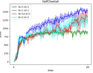
Ensemble Size and Planning Depth
In this section, we investigate how the ensemble sizeNand the planning depthdin ACE influence the performance. We performed experiments in HalfCheetah with variousN and
dand used the same evaluation protocol as before. As a large
Nanddinduced a significant computation increase, we only
usedN up to 10 anddup to 2. The results are reported in Figure 2.
To summarize,N = 5andd = 1achieved the best per-formance. We hypothesize there is a trade-off in the selec-tion of both the ensemble size and the planning depth. On the one hand, a single actor can easily be trapped into local maxima during training. The more actors we have, the more likely we find the global maxima. On the other hand, all the actors share the same encoding function with the critic. A large number of actors may dominate the training of the en-coding function to damage the critic learning. So a medium ensemble size is likely to achieve the best performance. A possible solution is to normalize the gradient according to the ensemble size, and we leave this for future work. With a perfect model, the more planning steps we have, the more accurateQestimation we can get. However, with a learned value prediction model, there is a compound error in un-rolling. So a medium planning depth is likely to achieve the best performance. Similar phenomena were also observed in the multi-step Dyna planning (Yao et al. 2009).
Figure 2: Evaluation curves of ACE in HalfCheetah with dif-ferentN andd. Each curve is averaged over 5 independent runs, and standard errors are plotted in shadow.
Related Work
intra-ACE ACE-Alt TM-ACE Ensemble-DDPG Shared-DDPG Wide-DDPG DDPG Ant 1041(70.8) 983(36.8) 1031(55.6) 1026(87.2) 796(16.8) 871(19.9) 875(14.2) HalfCheetah 1667(40.4) 1023(60.4) 800(28.8) 812(49.4) 771(79.6) 733(52.5) 703(37.3) Hopper 2136(86.4) 1923(88.3) 1586(85.0) 1972(63.4) 2047(76.7) 2090(118.6) 2133(99.0) Humanoid 380(56.1) 441(90.1) 61(6.8) 76(11.4) 53(2.2) 54(1.0) 54(1.7)
HF 311(30.3) 289(20.8) 126(39.6) 85(5.6) 53(1.0) 55(1.6) 53(1.4) HFH 22(2.4) 20(2.2) -4(2.1) 2(7.5) 6(6.4) 15(3.2) 15(2.5)
IDP 7555(1610.9) 9356(1.1) 7549(1613.7) 4102(1923.2) 7549(1613.6) 7548(1618.7) 5662(1945.9) IP 417(212.8) 1000(0.0) 415(213.4) 1000(0.0) 1000(0.0) 1000(0.0) 1000(0.0) IPS 892(0.1) 892(0.2) 891(0.2) 891(0.2) 891(0.4) 546(308.7) 891(0.4)
Pong 12(0.3) 11(0.1) 6(0.7) 8(0.9) 4(0.2) 4(0.1) 5(0.8)
Reacher 16(0.7) 17(0.2) 17(0.5) 17(0.3) 20(0.7) 15(2.2) 18(0.9) Walker2d 1659(65.9) 1864(21.4) 1086(97.0) 1142(99.5) 1142(146.3) 1185(121.2) 815(11.4)
Table 1: Best evaluation performance during training. Mean and standard error are reported. Bold numbers indicate the best performance. Scores are averaged over 5 independent runs. Numbers are rounded for the ease of display. HF, HFH, IDP, IP, and IPS stand for HumanoidFlagrun, HumanoidFlagrunHarder, InvertedDoublePendulum, InvertedPendulum, and InvertedPendu-lumSwingup respectively.
option policy was trained via a policy search method. In ACE, we consider deterministic intra-option policies, and the intra-option policies are optimized under the same ob-jective as OCA.
Gu et al. (2016) parameterized theQfunction in a quadric form to deal with continuous control problems. In this way, the global maxima can be determined analytically. However, in general, the optimalQvalue does not necessarily fall into this quadric form. In ACE, we use an actor ensemble to search the global maxima of theQfunction. Gu et al. (2016) utilized a transition model to generate imaginary data, which is orthogonal to ACE.
Ensemble in RL Wiering and Van Hasselt (2008) de-signed four ensemble methods combining five RL algo-rithms with a voting scheme based on value functions of different RL algorithms. Hans and Udluft (2010) used a net-work ensemble to improve the performance of Fitted Q-Iteration. Osband et al. (2016) used a Q ensemble to ap-proximate Thomas’ sampling, resulting in improved explo-ration and performance boost in challenging video games. Huang et al. (2017) used both an actor ensemble and a critic ensemble in continuous control problems. However, to our best knowledge, the present work is the first to relate ensem-ble with options and to use an ensemensem-ble for a look-ahead tree search in continuous control problems.
Closing Remarks
In this paper, we propose the ACE algorithm for continu-ous control problems. From an ensemble perspective, ACE utilizes an actor ensemble to search the global maxima of a critic function. From an option perspective, ACE is a spe-cial option-critic algorithm with deterministic intra-option policies. Thanks to the actor ensemble, ACE is able to per-form a look-ahead tree search with a learned value predic-tion model in continuous control problems, resulting in a significant performance boost in challenging robot manipu-lation tasks.
Acknowledgement
Due to a technical mistake in submission, we failed to input the whole author list in this camera-ready version, which should be Shangtong Zhang, Hao Chen, Hengshuai Yao. The authors thank Bo Liu for feedbacks of the first draft of this paper. We also appreciate the insightful reviews of the anonymous reviewers.
References
Bacon, P.-L.; Harb, J.; and Precup, D. 2017. The option-critic architecture. InProceedings of the 31st AAAI Confer-ence on Artificial IntelligConfer-ence.
Barth-Maron, G.; Hoffman, M. W.; Budden, D.; Dabney, W.; Horgan, D.; Muldal, A.; Heess, N.; and Lillicrap, T. 2018. Distributed distributional deterministic policy gradi-ents.arXiv preprint arXiv:1804.08617.
Browne, C. B.; Powley, E.; Whitehouse, D.; Lucas, S. M.; Cowling, P. I.; Rohlfshagen, P.; Tavener, S.; Perez, D.; Samothrakis, S.; and Colton, S. 2012. A survey of monte carlo tree search methods. IEEE Transactions on Computa-tional Intelligence and AI in Games.
Coulom, R. 2006. Efficient selectivity and backup operators in monte-carlo tree search. InProceedings of the Interna-tional Conference on Computers and Games.
Degris, T.; White, M.; and Sutton, R. S. 2012. Off-policy actor-critic. arXiv preprint arXiv:1205.4839.
Farquhar, G.; Rockt¨aschel, T.; Igl, M.; and Whiteson, S. 2018. Treeqn and atreec: Differentiable tree-structured models for deep reinforcement learning. arXiv preprint arXiv:1710.11417.
Gu, S.; Lillicrap, T.; Sutskever, I.; and Levine, S. 2016. Con-tinuous deep q-learning with model-based acceleration. In
Proceedings of the 33rd International Conference on Ma-chine Learning.
Huang, Z.; Zhou, S.; Zhuang, B.; and Zhou, X. 2017. Learning to run with actor-critic ensemble. arXiv preprint arXiv:1712.08987.
Klissarov, M.; Bacon, P.-L.; Harb, J.; and Precup, D. 2017. Learnings options end-to-end for continuous action tasks.
arXiv preprint arXiv:1712.00004.
Knuth, D. E., and Moore, R. W. 1975. An analysis of alpha-beta pruning.Artificial Intelligence.
Lillicrap, T. P.; Hunt, J. J.; Pritzel, A.; Heess, N.; Erez, T.; Tassa, Y.; Silver, D.; and Wierstra, D. 2015. Continuous control with deep reinforcement learning. arXiv preprint arXiv:1509.02971.
Lin, L.-J. 1992. Self-improving reactive agents based on reinforcement learning, planning and teaching. Machine Learning.
Mansley, C. R.; Weinstein, A.; and Littman, M. L. 2011. Sample-based planning for continuous action markov de-cision processes. InProceedings of the 21st International Conference on Automated Planning and Scheduling. Mnih, V.; Kavukcuoglu, K.; Silver, D.; Rusu, A. A.; Veness, J.; Bellemare, M. G.; Graves, A.; Riedmiller, M.; Fidjeland, A. K.; Ostrovski, G.; et al. 2015. Human-level control through deep reinforcement learning. Nature.
Nair, V., and Hinton, G. E. 2010. Rectified linear units improve restricted boltzmann machines. InProceedings of the 27th International Conference on Machine Learning. Nitti, D.; Belle, V.; and De Raedt, L. 2015. Planning in discrete and continuous markov decision processes by prob-abilistic programming. InProceedings of the 17th Joint Eu-ropean Conference on Machine Learning and Knowledge Discovery in Databases.
Oh, J.; Singh, S.; and Lee, H. 2017. Value prediction net-work. InAdvances in Neural Information Processing Sys-tems.
Osband, I.; Blundell, C.; Pritzel, A.; and Van Roy, B. 2016. Deep exploration via bootstrapped dqn. InAdvances in Neu-ral Information Processing Systems.
Silver, D.; Lever, G.; Heess, N.; Degris, T.; Wierstra, D.; and Riedmiller, M. 2014. Deterministic policy gradient algo-rithms. InProceedings of the 31st International Conference on Machine Learning.
Silver, D.; Huang, A.; Maddison, C. J.; Guez, A.; Sifre, L.; Van Den Driessche, G.; Schrittwieser, J.; Antonoglou, I.; Panneershelvam, V.; Lanctot, M.; et al. 2016. Mastering the game of go with deep neural networks and tree search.
Nature.
Sturtevant, N. 2008. An analysis of uct in multi-player games. InProceedings of the International Conference on Computers and Games.
Sutton, R. S.; McAllester, D. A.; Singh, S. P.; and Mansour, Y. 2000. Policy gradient methods for reinforcement learning with function approximation. InAdvances in Neural Infor-mation Processing Systems.
Sutton, R. S.; Precup, D.; and Singh, S. 1999. Between mdps and semi-mdps: A framework for temporal abstraction in reinforcement learning.Artificial Intelligence.
Sutton, R. S. 1990. Integrated architectures for learn-ing, plannlearn-ing, and reacting based on approximating dynamic programming. InProceedings of the 7th International Con-ference on Machine Learning.
Tassa, Y.; Doron, Y.; Muldal, A.; Erez, T.; Li, Y.; Casas, D. d. L.; Budden, D.; Abdolmaleki, A.; Merel, J.; Lefrancq, A.; et al. 2018. Deepmind control suite. arXiv preprint arXiv:1801.00690.
Tesauro, G. 1995. Temporal difference learning and td-gammon. Communications of the ACM.
Uhlenbeck, G. E., and Ornstein, L. S. 1930. On the theory of the brownian motion. Physical review.
Watkins, C. J., and Dayan, P. 1992. Q-learning. Machine Learning.
Weber, T.; Racani`ere, S.; Reichert, D. P.; Buesing, L.; Guez, A.; Rezende, D. J.; Badia, A. P.; Vinyals, O.; Heess, N.; Li, Y.; et al. 2017. Imagination-augmented agents for deep re-inforcement learning.arXiv preprint arXiv:1707.06203. Wiering, M. A., and Van Hasselt, H. 2008. Ensemble al-gorithms in reinforcement learning. IEEE Transactions on Systems, Man, and Cybernetics, Part B (Cybernetics). Yao, H.; Bhatnagar, S.; Diao, D.; Sutton, R. S.; and Szepesv´ari, C. 2009. Multi-step dyna planning for policy evaluation and control. InAdvances in Neural Information Processing Systems.