Differentiable Game Mechanics
Alistair Letcher∗ [email protected]
University of Oxford
David Balduzzi∗ [email protected]
DeepMind
S´ebastien Racani`ere [email protected] DeepMind
James Martens [email protected]
DeepMind
Jakob Foerster [email protected]
University of Oxford
Karl Tuyls [email protected]
DeepMind
Thore Graepel [email protected]
DeepMind
Editor:Kilian Weinberger
Abstract
Deep learning is built on the foundational guarantee that gradient descent on an objective function converges to local minima. Unfortunately, this guarantee fails in settings, such as generative adversarial nets, that exhibit multiple interacting losses. The behavior of gradient-based methods in games is not well understood – and is becoming increasingly important as adversarial and multi-objective architectures proliferate. In this paper, we develop new tools to understand and control the dynamics inn-player differentiable games.
The key result is to decompose the game Jacobian into two components. The first, symmetric component, is related to potential games, which reduce to gradient descent on an implicit function. The second, antisymmetric component, relates toHamiltonian games, a new class of games that obey a conservation law akin to conservation laws in classical mechanical systems. The decomposition motivatesSymplectic Gradient Adjustment (SGA), a new algorithm for finding stable fixed points in differentiable games. Basic experiments show SGA is competitive with recently proposed algorithms for finding stable fixed points in GANs – while at the same time being applicable to, and having guarantees in, much more general cases.
Keywords: game theory, generative adversarial networks, deep learning, classical mechan-ics, hamiltonian mechanmechan-ics, gradient descent, dynamical systems
1. Introduction
A significant fraction of recent progress in machine learning has been based on applying gradient descent to optimize the parameters of neural networks with respect to an objective function. The objective functions are carefully designed to encode particular tasks such as
c
supervised learning. A basic result is that gradient descent converges to a local minimum of the objective function under a broad range of conditions (Lee et al., 2017). However, there is a growing set of algorithms that do not optimize a single objective function, including: generative adversarial networks (Goodfellow et al., 2014; Zhu et al., 2017), proximal gradient TD learning (Liu et al., 2016), multi-level optimization (Pfau and Vinyals, 2016), synthetic gradients (Jaderberg et al., 2017), hierarchical reinforcement learning (Wayne and Abbott, 2014; Vezhnevets et al., 2017), intrinsic curiosity (Pathak et al., 2017; Burda et al., 2019), and imaginative agents (Racani`ere et al., 2017). In effect, the models are trained via games played by cooperating and competing modules.
The time-average of iterates of gradient descent, and other more general no-regret algorithms, are guaranteed to converge to coarse correlated equilibria in games (Stoltz and Lugosi, 2007). However, the dynamics do not converge to Nash equilibria – and do not even stabilize in general (Mertikopoulos et al., 2018; Papadimitriou and Piliouras, 2018). Concretely, cyclic behaviors emerge even in simple cases, see example 1.
This paper presents an analysis of the second-order structure of game dynamics that allows to identify two classes of games, potential and Hamiltonian, that are easy to solve separately. We then derive symplectic gradient adjustment1 (SGA), a method for finding stable fixed points in games. SGA’s performance is evaluated in basic experiments.
1.1. Background and Problem Description
Tractable algorithms that converge to Nash equilibria have been found for restricted classes of games: potential games, two-player zero-sum games, and a few others (Hart and Mas-Colell, 2013). Finding Nash equilibria can be reformulated as a nonlinear complementarity problem, but these are ‘hopelessly impractical to solve’ in general (Shoham and Leyton-Brown, 2008) because the problem is PPAD hard (Daskalakis et al., 2009).
Players are primarily neural nets in our setting. For computational reasons we restrict to gradient-based methods, even though game-theorists have considered a much broader range of techniques. Losses are not necessarily convex in any of their parameters, so Nash equilibria are not guaranteed to exist. Even leaving existence aside, finding Nash equilibria in nonconvex games is analogous to, but much harder than, finding global minima in neural nets – which is not realistic with gradient-based methods.
There are at least three problems with gradient-based methods in games. Firstly, the potential existence of cycles (recurrent dynamics) implies there are no convergence guarantees, see example 1 below and Mertikopoulos et al. (2018). Secondly, even when gradient descent converges, the rate of convergence may be too slow in practice because ‘rotational forces’ necessitate extremely small learning rates, see Figure 4. Finally, since there is no single objective, there is no way to measure progress. Concretely, the losses obtained by the generator and the discriminator in GANs are not useful guides to the quality of the images generated. Application-specific proxies have been proposed, for example the inception score for GANs (Salimans et al., 2016), but these are of little help during training. The inception score is domain specific and is no substitute for looking at samples. This paper tackles the first two problems.
1.2. Outline and Summary of Main Contributions
1.2.1. The Infinitesimal Structure of Games
We start with the basic case of a zero-sum bimatrix game: example 1. It turns out that the dynamics under simultaneous gradient descent can be reformulated in terms of Hamilton’s equations. The cyclic behavior arises because the dynamics live on the level sets of the Hamiltonian. More directly useful, gradient descent on the Hamiltonian converges to a Nash equilibrium.
Lemma 1 shows that the Jacobian of any game decomposes into symmetric and antisym-metric components. There are thus two ‘pure’ cases corresponding to when the Jacobian is symmetric and anti-symmetric. The first case, known as potential games (Monderer and Shapley, 1996), have been intensively studied in the game-theory literature because they are exactly the games where gradient descentdoes converge.
The second case, Hamiltonian2 games, were not studied previously, probably because they coincide with zero-sum games in the bimatrix case (or constant-sum, depending on the constraints). Zero-sum and Hamiltonian games differ when the losses are not bilinear or when there are more than two players. Hamiltonian games are important because (i) they are easy to solve and (ii) general games combine potential-like and Hamiltonian-like dynamics. Unfortunately, the concept of a zero-sum game is too loose to be useful when there are many players: any n-player game can be reformulated as a zero-sum (n+ 1)-player game where
`n+1=−Pni=1`i. In this respect, zero-sum games are as complicated as general-sum games. In contrast, Hamiltonian games are much simpler than general-sum games. Theorem 4 shows that Hamiltonian games obey a conservation law – which also provides the key to solving them, by gradient descent on the conserved quantity.
1.2.2. Algorithms
The general case, neither potential nor Hamiltonian, is more difficult and is therefore the focus of the remainder of the paper. Section 3 proposes symplectic gradient adjustment (SGA), a gradient-based method for finding stable fixed points in general games. Appendix A contains TensorFlow code to compute the adjustment. The algorithm computes two Jacobian-vector products, at a cost of two iterations of backprop. SGA satisfies a few natural desiderata explained in Section 3.1: (D1) it is compatible with the original dynamics; and it is guaranteed to find stable equilibria in (D2) potential and (D3) Hamiltonian games.
For general games, correctly picking the sign of the adjustment (whether to add or subtract) is critical since it determines the behavior near stable and unstable equilibria. Section 2.4 defines stable equilibria and contrasts them with local Nash equilibria. Theorem 10 proves that SGA converges locally to stable fixed points for sufficiently small parameters (which we quantify via the notion of an additive condition number). While strong, this may be impractical or slow down convergence significantly. Accordingly, Lemma 11 shows how to set the sign so as to be attracted towards stable equilibria and repelled from unstable ones. Correctly aligning SGA allows higher learning rates and faster, more robust convergence, see Theorem 15. Finally, Theorem 17 tackles the remaining class of saddle fixed points by proving that SGA locally avoids strict saddles for appropriate parameters.
1.2.3. Experiments
We investigate the empirical performance of SGA in four basic experiments. The first exper-iment shows how increasing alignment allows higher learning rates and faster convergence, Figure 4. The second set of experiments compares SGA with optimistic mirror descent on two-player and four-player games. We find that SGA converges over a much wider range of learning rates.
The last two sets of experiments investigate mode collapse, mode hopping and the related, less well-known problem of boundary distortion identified in Santurkar et al. (2018). Mode collapse and mode hopping are investigated in a setup involving a two-dimensional mixture of 16 Gaussians that is somewhat more challenging than the original problem introduced in Metz et al. (2017). Whereas simultaneous gradient descent completely fails, our symplectic adjustment leads to rapid convergence – slightly improved by correctly choosing the sign of the adjustment.
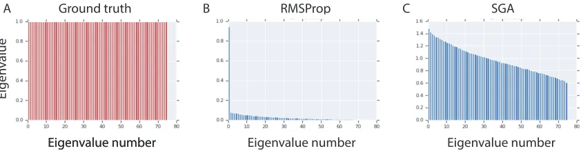
Finally, boundary distortion is studied using a 75-dimensional spherical Gaussian. Mode collapse is not an issue since there the data distribution is unimodal. However, as shown in Figure 10, a vanilla GAN with RMSProp learns only one of the eigenvalues in the spectrum of the covariance matrix, whereas SGA approximately learns all of them.
The appendix provides some background information on differential and symplectic geometry, which motivated the developments in the paper. The appendix also explores what happens when the analogy with classical mechanics is pushed further than perhaps seems reasonable. We experiment with assigning units (in the sense of masses and velocities) to quantities in games, and find that type-consistency yields unexpected benefits.
1.3. Related Work
Nash (1950) was only concerned with existence of equilibria. Convergence in two-player games was studied in Singh et al. (2000). WoLF (Win or Learn Fast) converges to Nash equilibria in two-player two-action games (Bowling and Veloso, 2002). Extensions include weighted policy learning (Abdallah and Lesser, 2008) and GIGA-WoLF (Bowling, 2004). Infinitesimal Gradient Ascent (IGA) is a gradient-based approach that is shown to converge to pure Nash equilibria in two-player two-action games. Cyclic behaviour may occur in case of mixed equilibria. Zinkevich (2003) generalised the algorithm to n-action games called GIGA. Optimistic mirror descent approximately converges in two-player bilinear zero-sum games (Daskalakis et al., 2018), a special case of Hamiltonian games. In more general settings it converges to coarse correlated equilibria.
Convergence has also been studied in variousn-player settings, see Rosen (1965); Scutari et al. (2010); Facchinei and Kanzow (2010); Mertikopoulos and Zhou (2016). However, the recent success of GANs, where the players are neural networks, has focused attention on a much larger class of nonconvex games where comparatively little is known, especially in the
A
B
symplectic
rotation
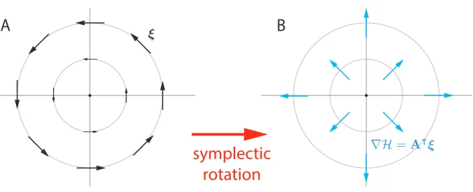
Figure 1: A minimal example of Hamiltonian mechanics. Consider a game where`1(x, y) =
xy,`2(x, y) =−xy, and the dynamics are given by ξ(x, y) = (y,−x). The game is a special case of example 1. (A) The dynamics ξ cycle around the origin since they live on the level sets of the HamiltonianH(x, y) = 12(x2+y2). (B)Gradient descent on the HamiltonianHconverges to the Nash equilibrium of the game, at the origin (0,0). Note thatA|ξ= (x, y) =∇H.
minimax motivated modifications to vanilla gradient descent have been investigated in the context of GANs, see Mertikopoulos et al. (2019); Gidel et al. (2018).
Learning with opponent-learning awareness (LOLA) infinitesimally modifies the objectives of players to take into account their opponents’ goals (Foerster et al., 2018). However, Letcher et al. (2019) recently showed that LOLA modifies fixed points and thus fails to find stable equilibria in general games.
Symplectic gradient adjustment was independently discovered by Gemp and Mahadevan (2018), who refer to it as “crossing-the-curl”. Their analysis draws on powerful techniques from variational inequalities and monotone optimization that are complementary to those developed here—see for example Gemp and Mahadevan (2016, 2017); Gidel et al. (2019). Using techniques from monotone optimization, Gemp and Mahadevan (2018) obtained more detailed and stronger results than ours, in the more particular case of Wasserstein LQ-GANs, where the generator is linear and the discriminator is quadratic (Feizi et al., 2017; Nagarajan and Kolter, 2017).
Network zero-sum games are shown to be Hamiltonian systems in Bailey and Piliouras (2019). The implications of the existence of invariant functions for games is just beginning
to be understood and explored.
1.3.1. Notation
Dot products are written as v|w or hv,wi. The angle between two vectors is θ(v,w). Positive definiteness is denotedS0.
2. The Infinitesimal Structure of Games
parameters. Our motivation is that we are primarily interested in use cases where players are interacting neural nets such as GANs (Goodfellow et al., 2014), a situation in which results from classical game theory do not straightforwardly apply.
Definition 1 (differentiable game)
A differentiable game consists in a set of players[n] ={1, . . . , n} and corresponding twice
continuously differentiable losses{`i :Rd→R}ni=1. Parameters are w= (w1, . . . ,wn)∈Rd
where Pn
i=1di =d. Player icontrols wi∈Rdi, and aims to minimize its loss.
It is sometimes convenient to writew= (wi,w−i) where w−i concatenates the parameters
of all the players other than the ith, which is placed out of order by abuse of notation.
Thesimultaneous gradient is the gradient of the losses with respect to the parameters of
the respective players:
ξ(w) = (∇w1`1, . . . ,∇wn`n)∈R d.
By the dynamicsof the game, we mean following thenegative of the vector field,−ξ, with infinitesimal steps. There is no reason to expect ξ to be the gradient of asingle function in general, and therefore no reason to expect the dynamics to converge to a fixed point.
2.1. Hamiltonian Mechanics
Hamiltonian mechanics is a formalism for describing the dynamics in classical physical systems, see Arnold (1989); Guillemin and Sternberg (1990). The system is described via canonical coordinates (q,p). For example,qoften refers to position andp to momentum of a particle or particles.
The Hamiltonian of the systemH(q,p) is a function that specifies the total energy as a function of the generalized coordinates. For example, in a closed system the Hamiltonian is given by the sum of the potential and kinetic energies of the particles. The time evolution of the system is given by Hamilton’s equations:
dq
dt = ∂H
∂p and
dp
dt =− ∂H
∂q.
An importance consequence of the Hamiltonian formalism is that the dynamics of the physical system—that is, the trajectories followed by the particles in phase space—live on the level sets of the Hamiltonian. In other words, the total energy is conserved.
2.2. Hamiltonian Mechanics in Games
The next example illustrates the essential problem with gradients in games and the key insight motivating our approach.
Example 1 (Conservation of energy in a zero-sum unconstrained bimatrix game)
Zero-sum games, where Pn
i=1`i ≡0, are well-studied. The zero-sum game
`1(x,y) =x|Ay and `2(x,y) =−x|Ay
has a Nash equilibrium at (x,y) = (0,0). The simultaneous gradientξ(x,y) = (Ay,−A|x)
The matrix A admits singular value decomposition (SVD) A = U|DV. Changing
to coordinates u = D12Ux and v = D
1
2Vy gives `1(u,v) = u|v and `2(u,v) = −u|v.
Introduce the Hamiltonian
H(u,v) = 1 2 kuk
2
2+kvk22
= 1 2(x
|U|DUx+y|V|DVy).
Remarkably, the dynamics can be reformulated via Hamilton’s equations in the coordinates
given by the SVD of A:
ξ(u,v) =
∂H
∂v,−
∂H ∂u
.
The vector field ξ cycles around the equilibrium because ξ conserves the Hamiltonian’s level
sets (i.e. hξ,∇Hi = 0). However, gradient descent on the Hamiltonian converges
to the Nash equilibrium. The remainder of the paper explores the implications and limitations of this insight.
Papadimitriou and Piliouras (2016) recently analyzed the dynamics of Matching Pennies (essentially, the above example) and showed that the cyclic behavior covers the entire parameter space. The Hamiltonian reformulation directly explains the cyclic behavior via a conservation law.
2.3. The Generalized Helmholtz Decomposition
The Jacobian of a game with dynamics ξ is the (d×d)-matrix of second-derivatives J(w) :=∇w·ξ(w)|=
∂ξα(w) ∂wβ
d
α,β=1, where ξα(w) is the α
th entry of the d-dimensional vectorξ(w). Concretely, the Jacobian can be written as
J(w) = ∇2
w1`1 ∇
2
w1,w2`1 · · · ∇
2
w1,wn`1 ∇2
w2,w1`2 ∇
2
w2`2 · · · ∇
2
w2,wn`2
..
. ...
∇2
wn,w1`n ∇
2
wn,w2`n · · · ∇
2
wn`n
where∇2
wi,wj`k is the (di×dj)-block of 2
nd-order derivatives. The Jacobian of a game is a square matrix, but not necessarily symmetric. Note: Greek indicesα, βrun overdparameter dimensions whereas Roman indicesi, j run overnplayers.
Lemma 1 (generalized Helmholtz decomposition)
The Jacobian of any vector field decomposes uniquely into two components J(w) =S(w) +
A(w) where S≡S| is symmetric and A+A|≡0 is antisymmetric.
Proof Any matrix decomposes uniquely as M = S+A where S = 12(M+M|) and A= 12(M−M|) are symmetric and antisymmetric. The decomposition is preserved by
orthog-onal change-of-coordinates: given orthogorthog-onal matrix P, we have P|MP=P|SP+P|AP since the terms remain symmetric and antisymmetric. Applying the decomposition to the Jacobian yields the result.
Definition 2 A game is a potential gameif the Jacobian is symmetric, i.e. if A(w)≡0.
It is aHamiltonian game if the Jacobian is antisymmetric, i.e. if S(w)≡0.
Potential games are well-studied and easy to solve. Hamiltonian games are a new class of games that are also easy to solve. The general case is more difficult, see Section 3.
2.4. Stable Fixed Points (SFPs) vs Local Nash Equilibria (LNEs)
There are (at least) two possible solution concepts in general differentiable games: stable fixed points and local Nash equilibria.
Definition 3 A point w is a local Nash equilibrium if, for all i, there exists a neighbor-hood Ui of wi such that`i(w0i,w−i)≥`i(wi,w−i) for w0i ∈Ui.
We introduce local Nash equilibria because finding global Nash equilibria is unrealistic in games involving neural nets. Gradient-based methods can reliably find local—but not global— optima of nonconvex objective functions (Lee et al., 2016, 2017). Similarly, gradient-based methods cannot be expected to find global Nash equilibria in nonconvex games.
Definition 4 A fixed point w∗ with ξ(w∗) = 0 is stable if J(w∗) 0 and J(w∗) is
invertible, unstable if J(w∗) ≺ 0 and a strict saddle if J(w∗) has an eigenvalue with
negative real part. Strict saddles are a subset of unstable fixed points.
The definition is adapted from Letcher et al. (2019), where conditions on the Jacobian hold at the fixed point; in contrast, Balduzzi et al. (2018a) imposed conditions on the Jacobian in aneighborhood of the fixed point. We motivate this concept as follows.
Positive semidefiniteness, J(w∗)0, is a minimal condition for any reasonable notion of stable fixed point. In the case of a single loss `, the Jacobian ofξ=∇`is the Hessian of `, i.e. J=∇2`. Local convergence of gradient descent on single functions cannot be guaranteed ifJ(w∗)0, since such points are strict saddles. These are almost always avoided by Lee
et al. (2017), so this semidefinite condition must hold.
Another viewpoint is that invertibility and positive semidefiniteness of the Hessian together imply positive definiteness, and the notion of stable fixed point specializes, in a one-player game, to local minima that are detected by the second partial derivative test. These minima are precisely those which gradient-like methods provably converge to. Stable fixed points are defined by analogy, though note that invertibility and semidefiniteness do
not imply positive definiteness inn-player games sinceJmay not be symmetric.
Finally, it is important to impose only positive semi-definiteness to keep the class as large as possible. Imposing strict positivity would imply that the origin is not an SFP in the cyclic game `1=xy=−`2 from Example 1, while clearly deserving of being so. Remark 1 The conditions J(w∗) 0 and J(w∗)≺0 are equivalent to the conditions on
the symmetric componentS(w∗)0 and S(w∗)≺0 respectively, since
u|Ju=u|Su+u|Au=u|Su
Stable fixed points and local Nash equilibria are both appealing solution concepts, one from the viewpoint of optimisation by analogy with single objectives, and the other from game theory. Unfortunately, neither is a subset of the other:
Example 2 (stable =6⇒ local Nash)
Let `1(x, y) =x3+xy and `2(x, y) =−xy. Then
ξ(x, y) =
3x2+y
−x
and J(x, y) =
6x 1
−1 0
.
There is a stable fixed point with invertible Hessian at (x, y) = (0,0), since ξ(0,0) = 0and
J(0,0)0 invertible. However any neighbourhood of x= 0 contains some small >0 for
which `1(−,0) =−3<0 =`1(0,0), so the origin is not a local Nash equilibrium.
Example 3 (local Nash =6⇒ stable)
Let `1(x, y) =`2(x, y) =xy. Then
ξ(x, y) =
y x
and J(x, y) =
0 1 1 0
.
There is a fixed point at (x, y) = (0,0) which is a local (in fact, global) Nash equilibrium
since `1(0, y) = 0≥`1(0,0)and `2(x,0) = 0≥`2(0,0)for all x, y∈R. However J=S has
eigenvaluesλ1 = 1 and λ2 =−1<0, so (0,0)is not a stable fixed point.
In Example 3, the Nash equilibrium is a saddle point of the common loss `=xy. Any algorithm that converges to Nash equilibria will thus converge to an undesirable saddle point. This rules out local Nash equilibrium as a solution concept for our purposes. Conversely, Example 2 emphasises the better notion of stability whereby player 1 may have a local incentive to deviate from the origin immediately, but would later be punished for doing so since the game is locally dominated by the ±xy terms, whose only ‘resolution’ or ‘stable minimum’ is the origin (see Example 1).
2.5. Potential Games
Potential games were introduced by Monderer and Shapley (1996). It turns out that our definition of potential game above coincides with a special case of the potential games of Monderer and Shapley (1996), which they refer to as exact potential games.
Definition 5 (classical definition of potential game)
A game is a potential game if there is a single potential functionφ:Rd→Rand positive
numbers {αi>0}n
i=1 such that
φ(wi0,w−i)−φ(wi00,w−i) =αi
`i(wi0,w−i)−`i(wi00,w−i)
for all iand all w0i,w00i,w−i, see Monderer and Shapley (1996).
Lemma 2 A game is a potential game iff αi∇wi`i=∇wiφ for all i, which is equivalent to
αi∇2w
iwj`i =αj∇
2
wiwj`j =αj
∇2w jwi`j
|
Proof See Monderer and Shapley (1996).
Corollary 3 Ifαi = 1for allithen Equation (1)is equivalent to requiring that the Jacobian
of the game is symmetric.
Proof In an exact potential game, the Jacobian coincides with the Hessian of the potential functionφ, which is necessarily symmetric.
Monderer and Shapley (1996) refer to the special case where αi = 1 for allias anexact
potential game. We use the shorthand ‘potential game’ to refer to exact potential games
in what follows.
Potential games have been extensively studied since they are one of the few classes of games for which Nash equilibria can be computed (Rosenthal, 1973). For our purposes, they are games where simultaneous gradient descent on the losses corresponds to gradient descent on a single function. It follows that descent onξ converges to a fixed point that is a local minimum of φor a saddle.
2.6. Hamiltonian Games
Hamiltonian games, where the Jacobian is antisymmetric, are a new class games. They are related to the harmonic games introduced in Candogan et al. (2011), see Section B.4. An example from Balduzzi et al. (2018b) may help develop intuition for antisymmetric matrices:
Example 4 (antisymmetric structure of tournaments)
Suppose n competitors play one-on-one and that the probability of player i beating player
j is pij. Then, assuming there are no draws, the probabilities satisfy pij +pji = 1 and
pii = 12. The matrix A =
log pij
1−pij n
i,j=1 of logits is then antisymmetric. Intuitively,
antisymmetry reflects a hyperadversarial setting where all pairwise interactions between
players are zero-sum.
Hamiltonian games are closely related to zero-sum games.
Example 5 (an unconstrained bimatrix game is zero-sum iff it is Hamiltonian)
Consider bimatrix game with `1(x,y) =x|Py and `2(x,y) =x|Qy, but where the
parame-ters are not constrained to the probability simplex. Thenξ= (Py,Q|x) and the Jacobian
components have block structure
A= 1 2
0 P−Q
(Q−P)| 0
and S= 1
2
0 P+Q
(P+Q)| 0
The game is Hamiltonian iff S= 0 iff P+Q= 0 iff `1+`2 = 0.
Example 6 (Hamiltonian game that is not zero-sum)
Fix constants a andb and suppose players 1 and 2 minimize losses
`1(x, y) =x(y−b) and `2(x, y) =−(x−a)y
with respect tox andy respectively.
Example 7 (zero-sum game that is not Hamiltonian)
Players 1 and 2 minimize
`1(x, y) =x2+y2 `2(x, y) =−(x2+y2).
The game actually has potential function φ(x, y) =x2−y2.
Hamiltonian games are quite different from potential games. In a Hamiltonian game there is a Hamiltonian functionHthat specifies a conserved quantity. In potential games the dynamics
equal ∇φ; in Hamiltonian games the dynamics areorthogonal to ∇H. The orthogonality
implies the conservation law that underlies the cyclic behavior in example 1.
Theorem 4 (conservation law for Hamiltonian games)
Let H(w) := 12kξ(w)k2
2. If the game is Hamiltonian then
i) ∇H =A|ξ and
ii) ξ preserves the level sets of Hsince hξ,∇Hi= 0.
iii) If the Jacobian is invertible and limkwk→∞H(w) = ∞ then gradient descent on H
converges to a stable fixed point.
Proof Direct computation shows ∇H = J|ξ for any game. The first statement follows sinceJ=Ain Hamiltonian games.
For the second statement, the directional derivative is DξH=hξ,∇Hi=ξ|A|ξ where
ξ|A|ξ= (ξ|A|ξ)|=ξ|Aξ =−(ξ|A|ξ) since A=−A| by anti-symmetry. It follows that ξ|A|ξ= 0.
For the third statement, gradient descent on H will converge to a point where ∇H= J|ξ(w) = 0. If the Jacobian is invertible then clearlyξ(w) = 0. The fixed-point is stable since 0≡S0 in a Hamiltonian game, recall remark 1.
In fact, His a Hamiltonian function for the game dynamics, see appendix B for a concise explanation. We use the notation H(w) = 12kξ(w)k2 throughout the paper. However, H can only be interpreted as a Hamiltonian function forξ when the game is Hamiltonian.
3. Algorithms
We have seen that fixed points of potential and Hamiltonian games can be found by descent onξ and∇H respectively. This Section tackles finding stable fixed points in general games.
3.1. Finding Stable Fixed Points
There are two classes of games where we know how to find stable fixed points: potential games where ξ converges to a local minimum and Hamiltonian games where∇H, which is orthogonal to ξ, finds stable fixed points.
In the general case, the following desiderata provide a set of reasonable properties for an adjustment ξλ of the game dynamics. Recall thatθ(u,v) is the angle between the vectors u and v.
3.1.1. Desiderata
To find stable fixed points, an adjustment ξλ to the game dynamics should satisfy
D1. compatible3 with game dynamics: hξλ,ξi=α1· kξk2;
D2. compatible with potential dynamics:
if the game is a potential game then hξλ,∇φi=α2· k∇φk2;
D3. compatible with Hamiltonian dynamics:
If the game is Hamiltonian then hξλ,∇Hi=α3· k∇Hk2;
D4. attracted to stable equilibria:
in neighborhoods where S0, require θ(ξλ,∇H)≤θ(ξ,∇H);
D5. repelled by unstable equilibria:
in neighborhoods where S≺0, require θ(ξλ,∇H)≥θ(ξ,∇H).
for someα1, α2, α3 >0.
Desideratum D1 does not guarantee that players act in their own self-interest—this requires a stronger positivity condition on dot-products with subvectors of ξ, see Balduzzi (2017). DesiderataD2 andD3 imply that the adjustment behaves correctly in potential and
Hamiltonian games respectively.
To understand desiderata D4 and D5, observe that gradient descent on H = 12kξk2 will find local minima that are fixed points of the dynamics. However, we specifically wish to converge to stable fixed points. DesideratumD4 and D5 require that the adjustment improves the rate of convergence to stable fixed points (by finding a steeper angle of descent), and avoids unstable fixed points.
More concretely, desiderata D4 can be interpreted as follows. If ξ points at a stable equilibrium then we require that ξλ points more towards the equilibrium (i.e. has smaller angle). Conversely, desiderataD5 requires that ifξ points away then the adjustment should point further away.
The unadjusted dynamics ξ satisfies all the desiderata except D3.
3.2. Consensus Optimization
Since gradient descent on the functionH(w) = 12kξk2finds stable fixed points in Hamiltonian games, it is natural to ask how it performs in general games. If the JacobianJ(w) is invertible, then∇H=J|ξ= 0 iff ξ= 0. Thus, gradient descent onHconverges to fixed points of ξ.
However, there is no guarantee that descent onHwill find astablefixed point. Mescheder et al. (2017) proposeconsensus optimization, a gradient adjustment of the form
ξ+λ·J|ξ =ξ+λ· ∇H.
Unfortunately, consensus optimization can converge to unstable fixed points even in simple cases where the ‘game’ is to minimize a single function:
Example 8 (consensus optimization can converge to a global maximum)
Consider a potential game with losses `1(x, y) =`2(x, y) =−2κ(x2+y2) withκ0. Then
ξ=−κ·
x y
and J=−
κ 0 0 κ
Note that kξk2 =κ2(x2+y2) and
ξ+λ·J|ξ =κ(λκ−1)·
x y
.
Descent on ξ+λ·J|ξ converges to the global maximum(x, y) = (0,0)unless λ < 1κ.
Although consensus optimization works well in two-player zero-sum, it cannot be considered a candidate algorithm for finding stable fixed points in general games since it fails in the basic case of potential games. Consensus optimization only satisfies desiderataD3 andD4.
3.3. Symplectic Gradient Adjustment
The problem with consensus optimization is that it can perform worse than gradient descent on potential games. Intuitively, it makes bad use of the symmetric component of the Jacobian. Motivated by the analysis in Section 2, we propose symplectic gradient adjustment, which takes care to only use the antisymmetric component of the Jacobian when adjusting the dynamics.
Proposition 5 The symplectic gradient adjustment (SGA)
ξλ:=ξ+λ·A|ξ.
satisfies D1—D3 for λ >0, with α1 = 1 =α2 and α3=λ.
Proof First claim: λ·ξ|A|ξ = 0 by anti-symmetry of A. Second claim: A ≡ 0 in a potential game, so ξλ = ξ = ∇φ. Third claim: hξλ,∇Hi = hξλ,J|ξi = hξλ,A|ξi =
λ·ξ|AA|ξ =λ· k∇Hk2 sinceJ=Aby assumption.
3.4. Convergence
We begin by analysing convergence of SGA near stable equilibria. The following lemma highlights that the interaction between the symmetric and antisymmetric components is important for convergence. Recall that two matrices A and S commute iff [A,S] := AS−SA=0. That is,A andS commute iffAS=SA. Intuitively, two matrices commute if they have the same preferred coordinate system.
Lemma 6 If S 0 is symmetric positive semidefinite and S commutes with A then ξλ
points towards stable fixed points for non-negativeλ:
hξλ,∇Hi ≥0 for all λ≥0.
Proof First observe that ξ|ASξ = ξ|S|A|ξ =−ξ|SAξ, where the first equality holds since the expression is a scalar, and the second holds sinceS=S|and A=−A|. It follows thatξ|ASξ = 0 if SA=AS. Finally rewrite the inequality as
hξλ,∇Hi=hξ+λ·A|ξ,Sξ+A|ξi=ξ|Sξ+λξ|AA|ξ ≥0
sinceξ|ASξ= 0 and by positivity of S,λand AA|.
The lemma suggests that in general the failure of A and S to commute should be important for understanding the dynamics of ξλ. We therefore introduce the additive condition number κ to upper-bound the worst-case noncommutativity ofS, which allows to quantify the relationship betweenξλ and∇H. If κ= 0, thenS=σ·I commutes withall
matrices. The larger the additive condition number κ, the larger thepotential failure of S to commute with other matrices.
Theorem 7 LetSbe a symmetric matrix with eigenvaluesσmax≥ · · · ≥σmin. Theadditive
condition number4 ofS is κ:=σmax−σmin. If S0 is positive semidefinite with additive
condition number κ thenλ∈(0,κ4) implies
hξλ,∇Hi ≥0.
If S is negative semidefinite, thenλ∈(0,4κ) implies
hξ−λ,∇Hi ≤0.
The inequalities are strict if Jis invertible.
Proof We prove the case S0; the caseS0 is similar. Rewrite the inequality as
hξ+λ·A|ξ,∇Hi= (ξ+λ·A|ξ)|·(S+A|)ξ =ξ|Sξ+λξ|ASξ+λξ|AA|ξ
4. The condition number of a positive definite matrix is σmax
Letβ =kA|ξk and ˜S=S−σ
min·I, where Iis the identity matrix. Then ξ|Sξ+λξ|ASξ+λ·β2 ≥ξ|S˜ξ+λξ|AS˜ξ+λ·β2
since ξ|Sξ ≥ξ|S˜ξ by construction and ξ|AS˜ξ =ξ|ASξ−σminξ|Aξ = ξ|ASξ because ξ|Aξ = 0 by the anti-symmetry ofA. It therefore suffices to show that the inequality holds when σmin = 0 and κ=σmax.
Since S is positive semidefinite, there exists an upper-triangular square-root matrixT
such thatT|T=S and so ξ|Sξ =kTξk2. Further,
|ξ|ASξ| ≤ kA|ξk · kT|Tξk ≤√σmax· kA|ξk · kTξk. sincekTk2=
√
σmax. Putting the observations together obtains
kTξk2+λ(kAξk2− hAξ,Sξi)≥ kTξk2+λ(kAξk2− kAξk kSξk ≥ kTξk2+λkAξk(kAξk − kSξk)
≥ kTξk2+λkAξk(kAξk −√σmaxkTξk)
Setα=√λand η=√σmax. We can continue the above computation
kTξk2+λ(kAξk2− hAξ,Sξi)≥ kTξk2+α2kAξk(kAξk −ηkTξk) =kTξk2+α2kAξk2−α2kAξkηkTξk
= (kTξk −αkAξk)2+ 2αkAξk kTξk −α2ηkAξk kTξk
= (kTξk −αkAξk)2+kAξk kTξk(2α−α2η)
Finally, 2α−α2η >0 for any α in the range (0,2η), which is to say, for any 0< λ < σ4 max.
The kernel of S and the kernel ofT coincide. Ifξ is in the kernel of A, resp. T, it cannot be in the kernel ofT, resp. A and the term (kTξk −αkAξk)2 is positive. Otherwise, the termkAξkkTξkis positive.
The theorem above guarantees that SGA always points in the direction of stable fixed points for λ sufficiently small. This does not technically guarantee convergence; we use Ostrowski’s theorem to strengthen this formally. Applying Ostrowski’s theorem will require taking a more abstract perspective by encoding the adjusted dynamics into a differentiable mapF : Ω→Rd of the formF(w) =w−αξ
λ(w).
Theorem 8 (Ostrowski) LetF : Ω→Rdbe a continuously differentiable map on an open
subsetΩ⊆Rd, and assumew∗ ∈Ωis a fixed point. If all eigenvalues of ∇F(w∗) are strictly
in the unit circle ofC, then there is an open neighbourhood U ofw∗ such that for all w0 ∈U,
the sequence Fk(w0) of iterates ofF converges to w∗. Moreover, the rate of convergence is
at least linear in k.
Corollary 9 A matrix M is called positive stable if all its eigenvalues have positive real
part. Assume w∗ is a fixed point of a differentiable game such that (I+λA|)J(w∗) is
positive stable for λ in some setΛ. Then SGA converges locally to w∗ for λ∈Λ andα >0
sufficiently small.
Proof Let X= (I+λA|). By definition of fixed points, ξ(w∗) = 0 and so
∇[Xξ](w∗) =∇X(w∗)ξ(w∗) +X(w∗)∇ξ(w∗) =XJ(w∗)
is positive stable by assumption, namely has eigenvalues ak+ibk with ak > 0. Writing F(w) =w−αXξ(w) for the iterative procedure given by SGA, it follows that
∇F(w∗) =I−α∇[Xξ](w∗)
has eigenvalues 1−αak−iαbk, which are in the unit circle for smallα. More precisely,
|1−αak−iαbk|2 <1 ⇐⇒ 1−2αak+α2a2k+α2b2k<1 ⇐⇒ 0< α < 2ak
a2k+b2k
which is always possible for ak>0. Hence ∇F(w∗) has eigenvalues in the unit circle for 0< α <mink2ak/(a2k+b2k), and we are done by Ostrowski’s Theorem since w
∗ is a fixed
point ofF.
Theorem 10 Let w∗ be a stable fixed point and κ the additive condition number of S(w∗).
Then SGA converges locally to w∗ for all λ∈(0,4κ) and α >0 sufficiently small.
Proof By Theorem 5 and the assumption that w∗ is a stable fixed point with invertible Jacobian, we know that
hξλ,∇Hi=h(I+λA|)ξ,J|ξi>0
for λ∈(0,4κ). The proof does not rely on any particular property ofξ, and can trivially be extended to the claim that
h(I+λA|)u,J|ui>0
for all non-zero vectors u. In particular this can be rewritten as
u|J(I+λA|)ui>0,
which implies positive definiteness ofJ(I+λA|). A positive definite matrix is positive stable, and any matricesAB andBAhave identical spectrum. This implies also that (I+λA|)Jis positive stable, and we are done by the corollary above.
3.5. Picking sign(λ)
This section explains desiderata D4—D5 and shows how to pick sign(λ) to speed up convergence towards stable and away from unstable fixed points. In the example below, almost any choice of positive λ results in convergence to an unstable equilibrium. The problem arises from the combination of a weak repellor with a strong rotational force.
Example 9 (failure case for λ >0)
Suppose >0 is small and
`1(x, y) =−
2x
2−xy and `
2(x, y) =−
2y 2+xy
with an unstable equilibrium at (0,0). The dynamics are
ξ=·
−x −y + −y x
with A=
0 −1 1 0
and
A|ξ = x y + −y x
Finally observe that
ξ+λ·A|ξ = (λ−)·
x y
+ (1 +λ)·
−y x
which converges to the unstable equilibrium if λ > .
We now show how to pick the sign of λto avoid unstable equilibria. First, observe that
hξ,∇Hi=ξ|(S+A)|ξ =ξ|Sξ. It follows that for ξ6= 0:
(
if S0 thenhξ,∇Hi ≥0;
if S≺0 thenhξ,∇Hi<0. (2)
A criterion to probe the positive/negative definiteness ofSis thus to check the sign ofhξ,∇Hi. The dot product can take any value if S is neither positive nor negative (semi-)definite. The behavior near saddle points will be explored in Section 3.7.
Recall that desiderata D4 requires that, if ξ points at a stable equilibrium then we require thatξλ pointsmore towards the equilibrium (i.e. has smaller angle). Conversely, desiderata D5 requires that, ifξ points away then the adjustment should point further away. More formally,
Definition 6 Let uand vbe two vectors. The infinitesimal alignmentofξλ:=u+λ·v
with a third vector w is
align(ξλ,w) := d
dλ
cos2θλ |λ=0 for θλ :=θ(ξλ,w).
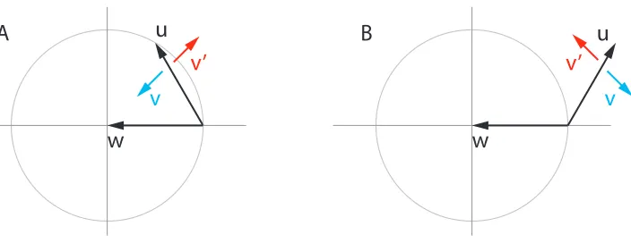
Ifu andwpoint the same way, u|w>0, then align>0 whenv bendsufurther toward w, see Figure 2A. Otherwise align>0 when vbends u away from w, see Figure 2B.
w
u
v
v’
w
u
v
v’
A
B
Figure 2: Infinitesimal alignment between u+λv and w is positive (cyan) when small positive λ either: (A) pulls u toward w, if w and u have angle <90◦; or (B) pushes u away from w if their angle is > 90◦. Conversely, the infinitesimal alignment is negative (red) when small positiveλeither: (A)pushesu away from wwhen their angle is acute or (B)pulls utoward wwhen their angle is obtuse.
Algorithm 1 Symplectic Gradient Adjustment Input: lossesL={`i}n
i=1, weightsW ={wi}ni=1 ξ ←
gradient(`i,wi) for (`i,wi)∈(L,W)
A|ξ←get sym adj(L,W) // appendix A
if alignthen
∇H ←
gradient(12kξk2,w) for w∈ W)
λ←sign
1
dhξ,∇HihA|ξ,∇Hi+
// = 101 else
λ←1 end if
Output: ξ+λ·A|ξ // plug into any optimizer
Lemma 11 When ξλ is the symplectic gradient adjustment,
sign
align(ξλ,∇H)
= sign
hξ,∇Hi · hA|ξ,∇Hi.
Proof Observe that
cos2θλ=
hξλ,∇Hi kξλk · k∇Hk
2
= hξ,∇Hi+ 2λhξ,∇HihA
|ξ,∇Hi+O(λ2)
kξk2+O(λ2)
· k∇Hk2
where the denominator has no linear term in λbecause ξ⊥A|ξ. It follows that the sign of the infinitesimal alignment is
sign
d dλcos
2θλ
= sign n
hξ,∇HihA|ξ,∇Hio
Intuitively, computing the sign of hξ,∇Hi provides a check for stable and unstable fixed points. Computing the sign ofhA|ξ,∇Hi checks whether the adjustment term points towards or away from the nearby fixed point. Putting the two checks together yields a prescription for the sign of λ, as follows.
Proposition 12 DesiderataD4—D5are satisfied forλsuch thatλ· hξ,∇Hi · hA|ξ,∇Hi ≥
0.
Proof If we are in a neighborhood of a stable fixed point then hξ,∇Hi ≥ 0. It follows by Lemma 11 that sign
align(ξλ),∇H)
= sign
hA|ξ,∇Hiand so choosing sign(λ) =
signhA|ξ,∇Hi leads to the angle between ξ
λ and ∇H being smaller than the angle
betweenξand∇H, satisfying desideratumD4. The proof for the unstable case is similar.
3.5.1. Alignment and Convergence Rates
Gradient descent is also known as the method of steepest descent. In general games, however, ξ does not follow the steepest path to fixed points due to the ‘rotational force’, which forces lower learning rates and slows down convergence.
The following lemma provides some intuition about alignment. The idea is that, the smaller the cosine between the ‘correct direction’wand the ‘update direction’ξ, the smaller the learning rate needs to be for the update to stay in a unit ball, see Figure 3.
Lemma 13 (Alignment Lemma)
Ifwandξare unit vectors with0<w|ξthenkw−η·ξk ≤1for0≤η ≤2w|ξ = 2 cosθ(w,ξ).
In other words, ensuring thatw−ηξ is closer to the origin than w requires smaller learning
rates η as the angle between w andξ gets larger.
Proof Check kw−η·ξk2= 1 +η2−2η·w|ξ≤1 iffη2 ≤2η·w|ξ. The result follows.
The next lemma is a standard technical result from the convex optimization literature.
Lemma 14 Let f : Rd → R be a convex Lipschitz smooth function satisfying k∇f(y)−
∇f(x)k ≤L· ky−xk for all x,y∈Rd. Then
|f(y)−f(x)− h∇f(x),y−xi| ≤ L
2 · ky−xk 2
for all x,y∈Rd.
Proof See Nesterov (2004).
w
w
A
B
Figure 3: Alignment and learning rates. The larger cosθ, the larger the learning rateη that can be applied to unit vectorξ without w+η·ξ leaving the unit circle.
Theorem 15 Supposef is convex and Lipschitz smooth withk∇f(x)−∇f(y)k ≤L·kx−yk.
Letwt+1=wt−η·vwherekvk=k∇f(wt)k. Then the optimal step size isη∗ = cosLθ where
θ:=θ(∇f(wt),v), with
f(wt+1)≤f(wt)−
cos2θ
2L · k∇f(wt)k
2.
The proof of Theorem 15 adapts Lemma 14 to handle the angle arising from the ‘rotational force’.
Proof By the Lemma 14,
f(y)≤f(x) +h∇f(x),y−xi+L
2ky−xk 2 =f(x)−η· h∇f,ξi+η2L
2 · kξk 2 =f(x)−η· h∇f,ξi+η2L
2 · k∇fk 2 =f(x)−η(α− η
2L)· k∇fk 2
where α:= cosθ. Solve
min
η ∆(η) = minη
n
−η(α− η
2L) o
to obtain η∗= Lα and ∆(η∗) =−α22Las required.
GR
ADIENT DESCENT
SGA
0.032 0.1
0.01 learning rate
Figure 4: SGA allows faster and more robust convergence to stable fixed points than vanilla gradient descent in the presence of ‘rotational forces’, by bending the direction of descent towards the fixed point. Note the gradient descent diverges extremely rapidly in the top-right panel, which has a different scale from the other panels.
3.6. Aligned Consensus Optimization
The stability criterion in Equation (2) also provides a simple way to prevent consensus optimization from converging to unstable equilibria. Aligned consensus optimizationis
ξ+|λ| ·signhξ,∇Hi·J|ξ, (3)
where in practice we set λ= 1. Aligned consensus optimization satisfies desiderataD3—D5. However, it behaves strangely in potential games. Multiplying by the Jacobian is the ‘inverse’ of Newton’s method since for potential games the Jacobian ofξ is the Hessian of the potential function. Multiplying by the Hessian increases the gap between small and large eigenvalues, increasing the (usual, multiplicative) condition number and slows down convergence. Nevertheless, consensus optimization works well in GANs (Mescheder et al., 2017), and aligned consensus may improve performance, see experiments below.
Dropping the first term ξ from Equation (3) yields a simpler update that also satisfies
LEARNING RATE LEARNING RATE
STEPS T
O
CONVER
GE
LOSS AFTER 250 STEPS
OMD SGA OMD
SGA
Figure 5: Comparison of SGA with optimistic mirror descent. The plots sweep over learning rates in range [0.01,1.75], withλ= 1 throughout for SGA. (Left): iterations to convergence, with maximum value of 250 after which the run was interrupted. (Right): average absolute value of losses over the last 10 iterations, 240-250, with
a cutoff at 5.
3.7. Avoiding Strict Saddles
How does SGA behave near saddles? We show that Symplectic Gradient Adjustment locally avoids strict saddles, provided that λandα are small and parameters are initialized with (arbitrarily small) noise. More precisely, letF(w) =w−αξλ(w) be the iterative optimization procedure given by SGA. Then every strict saddle w∗ has a neighbourhood U such that
{w∈U |Fn(w)→w∗ asn→ ∞} has measure zero for smallα >0 and λ.
Intuitively, the Taylor expansion around a strict saddle w∗ is locally dominated by the Jacobian at w∗, which has a negative eigenvalue. This prevents convergence to w∗ for random initializations of wnear w∗. The argument is made rigorous using the Stable Manifold Theorem following Lee et al. (2017).
Theorem 16 (Stable Manifold Theorem)
Let w∗ be a fixed point for the C1 local diffeomorphismF :U →Rd, where U is a
neighbour-hood of w∗ in Rd. Let Es⊕Eu be the generalized eigenspaces of ∇F(w∗) corresponding to
eigenvalues with|σ| ≤1and |σ|>1 respectively. Then there exists a local stable center
man-ifoldW with tangent space Esatw∗ and a neighbourhoodB ofw∗ such thatF(W)∩B ⊂W
and ∩∞n=0F−n(B)⊂W.
Proof See Shub (2000).
It follows that if∇F(w∗) has at least one eigenvalue |σ|>1 then Eu has dimension at least 1. Since W has tangent space Es atw∗ with codimension at least one, we conclude thatW has measure zero. This is central to proving that the set of nearby initial points which converge to a given strict saddlew∗ has measure zero. Sincewis initialized randomly, the following theorem is obtained.
Proof Let w∗ a strict saddle and recall that SGA is given by
F(w) =w−α(I−αJ)ξ(w).
All terms involved are continuously differentiable and we have
∇F(w∗) =I−α(I−αJ)J(w∗)
by assumption that ξ(w∗) = 0. Since all terms except I are of order at leastα, ∇F(w∗) is invertible for all α sufficiently small. By the inverse function theorem, there exists a neighbourhoodU ofw∗ such thatF is has a continuously differentiable inverse onU. Hence
F restricted to U is aC1 diffeomorphism with fixed point w∗.
By definition of strict saddles, J(w∗) has an eigenvalue with negative real part. It follows by continuity that (I−αJ)J(w∗) also has an eigenvaluea+ibwitha <0 forα sufficiently small. Finally,
∇F(w∗) =I−α(I−αJ)J(w∗)
has an eigenvalueσ = 1−αa−iαb with
|σ|= 1−2αa+α2(a2+b2)≥1−2αa >1.
It follows thatEs has codimension at least one, implying in turn that the local stable setW
has measure zero. We can now prove that
Z ={w∈U | lim
n→∞F
n(w) =w∗}
has measure zero, or in other words, that local convergence tow∗ occurs with zero probability. Let B the neighbourhood guaranteed by the Stable Manifold Theorem, and take any w∈Z. By definition of convergence there existsN ∈N such thatFN+n(w)∈B for alln∈N, so that
FN(w)∈ ∩∞n∈NF−n(B)⊂W
by the Stable Manifold Theorem. This implies that w ∈ F−N(W), and by extension w∈ ∪n∈NF
−n(W). Since wwas arbitrary, we obtain the inclusion
Z ⊆ ∪n∈NF
−n(W).
Now F−1 is C1, hence locally Lipschitz and thus preserves sets of measure zero, so that
F−n(W) has measure zero for each n. Countable unions of measure zero sets are still measure zero, so we conclude thatZ also has measure zero. In other words, SGA converges tow∗ with zero probability upon random initialization ofw inU.
Unlike stable and unstable fixed points, it is unclear how to avoid strict saddles using only alignment, that is, independently from the size ofλ.
4. Experiments
SYMPLECTIC GRADIENT ADJUSTMENT
OPTIMISTIC MIRROR DESCENT learning rate 1.0 learning rate 1.0
SYMPLECTIC GRADIENT ADJUSTMENT learning rate 0.4
SYMPLECTIC GRADIENT ADJUSTMENT learning rate 1.16
OPTIMISTIC MIRROR DESCENT learning rate 1.16 OPTIMISTIC MIRROR DESCENT
learning rate 0.4
4.1. Learning rates and alignment
We investigate the effect of SGA when a weak attractor is coupled to a strong rotational force:
`1(x, y) = 1 2x
2+ 10xy and `2(x, y) = 1 2y
2−10xy
Gradient descent is extremely sensitive to the choice of learning rate η, top row of Figure 4. As η increases through{0.01,0.032,0.1}gradient descent goes from converging extremely slowly, to diverging slowly, to diverging rapidly. SGA yields faster, more robust convergence. SGA converges faster with learning ratesη= 0.01 andη= 0.032, and only starts overshooting the fixed point forη = 0.1.
4.2. Basic adversarial games
Optimistic mirror descent is a family of algorithms that has nice convergence properties in games (Rakhlin and Sridharan, 2013; Syrgkanis et al., 2015). In the special case of optimistic
gradient descent the updates are
wt+1←wt−η·ξt−η·(ξt−ξt−1).
Figure 5 compares SGA with optimistic gradient descent (OMD) on a zero-sum bimatrix game with `1/2(w1,w2) =±w1|w2. The example is modified from Daskalakis et al. (2018) who also consider a linear offset that makes no difference. A run is taken to have converged if the average absolute value of losses on the last 10 iterations is < 0.01; we end each experiment after 250 steps.
The left panel shows the number of steps to convergence (when convergence occurs) over a range of learning rates. OMD’s peak performance is better than SGA, where the red curve dips below the blue. Howwever, we find that SGA converges—and does so faster—for a much wider range of learning rates. OMD diverges for learning rates not in the range [0.3, 1.2]. Simultaneous gradient descent oscillates without converging (not shown). The right panel shows the average performance of OMD and SGA on the last 10 steps. Once again, here SGA consistently performs better over a wider range of learning rates. Individual runs are shown in Figure 6.
4.2.1. OMD and SGA on a Four-Player Game
Figure 7 shows time to convergence (using the same convergence criterion as above) for optimistic mirror descent and SGA. The games are constructed with four players, each of which controls one parameter. The losses are
`1(w, x, y, z) =
2w
2+wx+wy+wz
`2(w, x, y, z) =−wx+
2x
2+xy+xz
`3(w, x, y, z) =−wy−xy+
2y 2+yz
`4(w, x, y, z) =−wz−xz−yz+ 2z
LEARNING RATE LEARNING RATE
STEPS T
O
CONVER
GE
STEPS T
O
CONVER
GE OMDSGA
OMD
SGA
WEAK
ATTRACTOR ATTRACTORNO
Figure 7: Time to convergence of OMD and SGA on two 4-player games. Times are cutoff after 5000 iterations. Left panel: Weakly positive definiteSwith= 1001 . Right panel: Symmetric component is identically zero.
where= 1001 in the left panel and= 0 in the right panel. The antisymmetric component of the game Jacobian is
A=
0 1 1 1
−1 0 1 1
−1 −1 0 1
−1 −1 −1 0
and the symmetric component is
S=·
1 0 0 0 0 1 0 0 0 0 1 0 0 0 0 1
.
OMD converges considerably slower than SGA across the full range of learning rates. It also diverges for learning rates >0.22. In contrast, SGA converges more quickly and robustly.
4.3. Learning a two-dimensional mixture of Gaussians
We apply SGA to a basic Generative Adversarial Network setup adapted from Metz et al. (2017). Data is sampled from a highly multimodal distribution designed to probe the
tendency of GANs to collapse onto a subset of modes during training. The distribution is a mixture of 16 Gaussians arranged in a 4×4 grid. Figure 8 shows the probability distribution that is sampled to train the generator and discriminator. The generator and discriminator networks both have 6 ReLU layers of 384 neurons. The generator has two output neurons; the discriminator has one.
Figure 8: Ground truth for GAN experiments on a two-dimensional mixture of 16 Gaussians.
The last two rows of Figure 9 show the performance of consensus optimization without and with alignment. Introducing alignment slightly improves speed of convergence (second column) and final result (fourth column), although intermediate results in third column are ambiguous.
Simultaneous gradient descent exhibits mode collapse followed by mode hopping in later iterations (not shown). Mode hopping is analogous to the cycles in example 1. Unaligned SGA converges to the correct distribution; alignment speeds up convergence slightly. Consensus optimization performs similarly in this GAN example. However, consensus optimization can converge to local maxima even in potential games, recall example 8.
4.4. Learning a high-dimensional unimodal Gaussian
Mode collapse is a well-known phenomenon in GANs. A more subtle phenomenon, termed boundary distortion, was identified in Santurkar et al. (2018). Boundary distortion is a form of covariate shift where the generator fails to model the true data distribution.
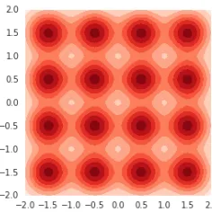
Santurkaret aldemonstrate boundary distortion using data sampled from a 75-dimensional unimodal Gaussian with spherical covariate matrix. Mode collapse is not a problem in this setting because the data distribution is unimodal. Nevertheless, they show that vanilla GANs fail to learn most of the spectrum of the covariate matrix.
Figure 10 reproduces their result. Panel A shows the ground truth: all 75 eigenvalues are equal to 1.0. Panel B shows the spectrum of the covariance matrix of the data generated by a GAN trained with RMSProp. The GAN concentrates on a single eigenvalue and essentially ignores the remaining 74 eigenvalues. This is similar to, but more extreme than, the empirical results obtained in Santurkar et al. (2018). We emphasize that the problem is not mode collapse, since the data is unimodal (although, it’s worth noting that most of the mass of a high-dimensional Gaussian lies on the “shell”).
GRADIENT DESCENT
4000 6000 8000
2000 Iteration:
SGA without ALIGNMENT
SGA with ALIGNMENT
CONSENSUS OPTIMIZATION
CONSENSUS OPTIMIZATION with ALIGNMENT
lear
ning r
at
e 9e
-5
lear
ning r
at
e 9e
-5
lear
ning r
at
e 9e
-5
lear
ning r
at
e 1e
-4
lear
ning r
at
e 9.25e
-5
Eigen
value
Eigenvalue number Eigenvalue number Eigenvalue number Eigenvalue number
Ground truth B RMSProp SGA
A C
Figure 10: Panel A: The ground truth is a 75 dimensional spherical Gaussian whose covariance matrix has all eigenvalues equal to 1.0. Panel B: A vanilla GAN trained with RMSProp approximately learns the first eigenvalue, but essentially ignores all the rest. Panel C: Applying SGA results in the GAN approximately learning all 75 eigenvalues, although the range varies from 0.6 to 1.5.
5. Discussion
Modern deep learning treats differentiable modules like plug-and-play lego blocks. For this to work, at the very least, we need to know that gradient descent will find local minima. Unfortunately, gradient descent does not necessarily find local minima when optimizing multiple interacting objectives. With the recent proliferation of algorithms that optimize more than one loss, it is becoming increasingly urgent to understand and control the dynamics of interacting losses. Although there is interesting recent work on two-player adversarial games such as GANs, there is essentially no work on finding stable fixed points in more general games played by interacting neural nets.
The generalized Helmholtz decomposition provides a powerful new perspective on game dynamics. A key feature is that the analysis is indifferent to the number of players. Instead, it is the interplay between the simultaneous gradientξ on the losses and the symmetric and antisymmetric matrices of second-order terms that guides algorithm design and governs the dynamics under gradient adjustments.
Symplectic gradient adjustment is a straightforward application of the generalized Helmholtz decomposition. It is unlikely that SGA is the best approach to finding stable fixed points. A deeper understanding of the interaction between the potential and Hamiltonian components will lead to more effective algorithms. Reinforcement learning algorithms that optimize multiple objectives are increasingly common, and second-order terms are difficult to estimate in practice. Thus, first-order methods that do not use Jacobian-vector products are of particular interest.
5.0.1. Gamification
player acting against its own self-interest by increasing its loss. We consider this acceptable insofar as it encourages convergence to a stable fixed point. The players are but a means to an end.
We have argued that stable fixed points are a more useful solution concept than local Nash equilibria for our purposes. However, neither is entirely satisfactory, and the question “What is the right solution concept for neural games?” remains open. In fact, it likely has many answers. The intrinsic curiosity module introduced by Pathak et al. (2017) plays two objectives against one another to drive agents to search for novel experiences. In this case, converging to a fixed point is precisely what is to be avoided.
It is remarkable—to give a few examples sampled from many—that curiosity, generating photorealistic images, and image-to-image translation (Zhu et al., 2017) can be formulated as games. What else can games do?
Acknowledgments
We thank Guillaume Desjardins and Csaba Szepesvari for useful comments.
Appendix A. TensorFlow Code to Compute SGA
Source code is available athttps://github.com/deepmind/symplectic-gradient-adjustment. Since computing the symplectic adjustment is quite simple, we include an explicit description here for completeness.
The code requires a list of n losses, Ls, and a list of variables for the n players, xs. The function fwd gradientswhich implements forward mode auto-differentiation is in the module tf.contrib.kfac.utils.
%compute Jacobian-vector product Jv def jac vec(ys,xs,vs) :
return fwd gradients(ys,xs,grad xs=vs,stop gradients=xs)
%compute Jacobian|-vector product J|v def jac tran vec(ys,xs,vs) :
dydxs=tf.gradients(ys,xs,grad ys=vs,stop gradients=xs) return [tf.zeros like(x) if dydx is None
else dydx for (x,dydx) in zip(xs,dydxs)]
%compute Symplectic Gradient Adjustment A|ξ
def get sym adj(Ls,xs) :
%compute game dynamics ξ
xi= [tf.gradients(`,x)[0] for (`,x) in zip(Ls,xs)] J xi=jac vec(xi,xs,xi)
At xi= [jt2−j for (j,jt) in zip(J xi,Jt xi)] return At xi
Appendix B. Helmholtz, Hamilton, Hodge, and Harmonic Games
This section explains the mathematical connections with the Helmholtz decomposition, symplectic geometry and the Hodge decomposition. The discussion is not necessary to understand the main text. It is also not self-contained. The details can be found in textbooks covering differential and symplectic geometry (Arnold, 1989; Guillemin and Sternberg, 1990; Bott and Tu, 1995).
B.1. The Helmholtz Decomposition
The classical Helmholtz decomposition states that any vector fieldξ in 3-dimensions is the sum of curl-free (gradient) and divergence-free (infinitesimal rotation) components:
ξ = ∇φ
|{z} gradient component
+ curl(B) | {z } rotational component
h
curl(•) :=∇ ×(•)i
We explain the link between curl and the antisymmetric component of the game Jacobian. Recall that gradients of functions are actually differential 1-forms, not vector fields. Differ-ential 1-forms and vector fields on a manifold are canonically isomorphic once a Riemannian metric has been chosen. In our case, we are implicitly using the Euclidean metric. The antisymmetric matrixAis the differential 2-form obtained by applying the exterior derivative
dto the 1-formξ.
In 3-dimensions, the Hodge star operator is an isormorphism from differential 2-forms to vector fields, and the curl can be reformulated as curl(•) =∗d(•). In claimingAis analogous to curl, we are simply dropping the Hodge-star operator.
Finally, recall that the Lie algebra of infinitesimal rotations in d-dimensions is given by antisymmetric matrices. When d = 3, the Lie algebra can be represented as vectors (three numbers specify a 3×3 antisymmetric matrix) with the×-product as Lie bracket. In general, the antisymmetric matrix Acaptures the infinitesimal tendency ofξ to rotate at each point in the parameter space.
B.2. Hamiltonian Mechanics
A symplectic form ω is a closed nondegenerate differential 2-form. Given a manifold with a symplectic form, a vector field ξ isHamiltonian vector field if there exists a function
H:M →Rsatisfying
ω(ξ,•) =dH(•) =h∇H,•i. (4)
The function is then referred to as the Hamiltonian function of the vector field. In our case, the antisymmetric matrix Ais a closed 2-form because A=dξ and d◦d= 0. It may however be degenerate. It is therefore a presymplectic form (Bottacin, 2005).
Setting ω=A, Equation (4) can be rewritten in our notation as
ω(ξ,•) | {z }
A|ξ
=dH(•) | {z } ∇H
justifying the terminology ‘Hamiltonian’.
B.3. The Hodge Decomposition
The exterior derivative dk: Ωk(M)→Ωk+1(M) is a linear operator that takes differential k-forms on a manifold M, Ωk(M), to differentialk+ 1-forms, Ωk+1(M). In the case k= 0, the exterior derivative is the gradient, which takes 0-forms (that is, functions) to 1-forms. Given a Riemannian metric, the adjoint of the exterior derivative δ goes in the opposite direction. Hodge’s Theorem states thatk-forms on a compact manifold decompose into a direct sum over three types:
Ωk(M) =dΩk−1(M)⊕Harmonick(M)⊕δΩk+1(M).
Setting k= 1, we recover a decomposition that closely resembles the generalized Helmholtz decomposition:
Ω1(M) | {z } 1-forms
= dΩ0(M) | {z } gradients of functions
⊕Harmk(M)⊕ δΩ2(M) | {z } antisymmetric component
The harmonic component is isomorphic to the de Rham cohomology of the manifold—which is zero when k= 1 and M =Rn.
Unfortunately, the Hodge decomposition does not straightforwardly apply to the case when M =Rn, since Rn is not compact. It is thus unclear how to relate the generalized
Helmholtz decomposition to the Hodge decomposition.
B.4. Harmonic and Potential Games
Candogan et al. (2011) derive a Hodge decomposition for games that is closely related in spirit to our generalized Helmholtz decomposition—although the details are quite different. Candogan et al. (2011) work with classical games (probability distributions on finite strategy sets). Their losses are multilinear, which is easier than our setting, but they have constrained solution sets, which is harder in many ways. Their approach is based on combinatorial Hodge theory (Jiang et al., 2011) rather than differential and symplectic geometry. Finding a best-of-both-worlds approach that encompasses both settings is an open problem.
Appendix C. Type Consistency
The next two sections carefully work through the units in classical mechanics and two-player games respectively. The third section briefly describes a use-case for type consistency.
C.1. Units in Classical Mechanics
Consider the well-known Hamiltonian
H(p, q) = 1 2
κ·q2+ 1
µ·p
whereq is position, p=µ·q˙ is momentum,µis mass, κ is surface tension andH measures energy. The units (denoted by τ) are
τ(q) =m τ(p) = kgs·m
τ(κ) = kgs2 τ(µ) =kg
where m is meters, kg is kilograms and s is seconds. Energy is measured in joules, and indeed it is easy to check thatτ(H) = kgs·m2 2.
Note that the units for differentation by x are τ(∂x∂ ) = τ(1x). For example, differentiating by time has units 1s. Hamilton’s equations state that ˙q= ∂H∂p = 1µ·p and ˙p=−∂H
∂q =−κ·q
where
τ( ˙q) = ms τ( ˙p) = kgs·2m
τ∂q∂= m1 τ∂p∂= kgs·m The resulting flow describing the dynamics of the system is
ξ= ˙q· ∂ ∂q + ˙p·
∂ ∂p =
1
µp· ∂
∂q −κq· ∂ ∂p
with unitsτ(ξ) = 1s. Hamilton’s equations can be reformulated more abstractly via symplectic geometry. Introduce the symplectic form
ω=dq∧dp with units τ(ω) = kg·m 2
s .
Observe that contracting the flow with the Hamiltonian obtains
ιξω =ω(ξ,•) =dH =
∂H ∂q ·dq+
∂H ∂p ·dp
with units τ(dH) =τ(H) = kgs·m2 2.
C.1.1. Losses in Classical Mechanics
Although there is no notion of “loss” in classical mechanics, it is useful (for the next section) to keep pushing the formal analogy. Define the “losses”
`1(q, p) = 1
µ·qp and `2(q, p) =−κ·qp (5)
with unitsτ(`1) = ms2 andτ(`2) = kg2s·3m2. The Hamiltonian dynamics can then be recovered
game-theoretically by differentiating`1 and `2 with respect toq and p respectively. It is easy to check that
ξ= ∂H
∂p ∂ ∂q −
∂H ∂q
∂ ∂p =
∂`1
∂q ∂ ∂q +
∂`2


![Figure 5: Comparison of SGA with optimistic mirror descent. The plots sweep over learningrates in range [0.01, 1.75], with λ = 1 throughout for SGA](https://thumb-us.123doks.com/thumbv2/123dok_us/9772290.1962415/22.612.116.489.95.219/figure-comparison-optimistic-mirror-descent-plots-sweep-learningrates.webp)