Symmetry Reductions of UT+U3UX +αUXXX X+βUY Y=0

International Journal of Mathematics Trends and Technology (IJMTT) – Volume 65 Issue 6 - June 2019

Symmetry Reductions of

U

_T

+ U

3

U

_X

+ αU

_XXX

_X

+ βU

_{Y Y}

= 0

1

J. K. Subashini , 2B. Mayil Vaganan 1

Department of Mathematics, K.L.N. College of Engineering, Pottapalayam-630612, India,

2

Department of Applied Mathematics and Statistics, Madurai Kamaraj University, Madurai-625021, Tamilnadu, India,

Abstract. A (2+1)-dimensional generalized KdV equation (ut+u3ux+αuxxx)x+βuyy =0, α, β∈ R+ is subjected to Lie’s classical method. Classification of its symmetry algebra into one- and two-dimensional subalgebras is carried out in order to facilitate its systematic reduction to (1+1) dimensional PDE and then to ODEs. A solution containing two arbitrary functions of time t is also determined.

Key words. A (2+1)-dimensional generalized KdV equation; Symmetry algebra.

1. introduction

The KdV equation

(1.1) 𝑢𝑡+ 𝑢𝑢𝑥+ 𝛿𝑢𝑥𝑥𝑥 = 0,

is integrable in the sense that it possesses solitons, B¨acklund transformations, Lax pair, infinite number of conservation laws and Painlev´e property. Whitham [7] has given a representation of a periodic wave as a sum of solitons for (1.1). Miura [4] established a relation between (1.1) and the modified KdV equation ut+au2ux+uxxx =0.

Liu and Yang [3] studied bifurcation problems for a generalized KdV equation (1.2) 𝑢𝑡+ 𝑎𝑢𝑛𝑢𝑥+ 𝑢𝑥𝑥𝑥 = 0, 𝑛 ≥ 1, 𝑎 ∈ 𝑅.

A generalized version of (1.2) in the form

(1.3) 𝑢𝑡+ 𝑢𝑛𝑢𝑥+ 𝛼(𝑡)𝑢 + 𝛽 𝑡 𝑢𝑥𝑥𝑥 = 0,

has recently been studied for its symmetry group and similarity solution by Senthilkumaran, Pandiaraja and Mayil Vaganan [6].

In this paper we introduce yet another (2 + 1)-dimensional variable coefficient KdV equation

(1.4) 𝑢𝑡+ 𝑢3𝑢𝑥+ 𝛼𝑢𝑥𝑥𝑥 𝑥 + 𝛽𝑢𝑦𝑦 = 0, 𝛼, 𝛽 ∈ 𝑅+.

Our intention is to show that equation (1.4) admits a five-dimensional Lie algebra, and classify it into the one- and two-dimensional sub algebras in order to reduce (1.4) to (1+1)-dimensional partial differential equations (PDEs) and then to ordinary differential equations (ODEs). It is shown that (1.4) reduces to a once differentiated generalized KdV equation, a linear equation 𝑊𝑟𝑟(𝑟, 𝑠) = 0. We shall establish that the symmetry

generators form a closed Lie algebra and this allowed us to use the recent method due to Ahmad, Bokhari, Kara and Zaman [1] to sucessively reduce (1.4) to (1+1)-dimensional PDEs and ODEs with the help of two-dimensional Abelian and solvable non-Abelian sub algebras.

ISSN: 2231-5373

http://www.ijmttjournal.org

Page 62

PDEs. In section 4 we show that the generators form a closed Lie algebra and use this fact to reduce (1.4) successively to (1+1)-dimensional PDEs and ODEs. Section 5 summarises the results of the present work.

2. The symmetry group and Lie algebra of (1.4)

If (1.4) is invariant under classical Lie group of infinitesimal transformations (Olver [5], Blumen and Kumei [2])

(2.1) 𝑥𝑖∗ = 𝑥𝑖+ 𝜖𝜉𝑖 𝑥, 𝑦, 𝑡, 𝑢 + 𝑂 𝜖2 , 𝑖 = 1,2,3,4,

where 𝜉1 = 𝜉, 𝜉2 = 𝜂, 𝜉3 = 𝜏, 𝜉4 = 𝜙, then the fourth prolongation pr(4)V of the

corresponding vector field

(2.2) 𝑉 = 𝜏 𝑥, 𝑦, 𝑡; 𝑢 𝜕𝑡+ 𝜉 𝑥, 𝑦, 𝑡; 𝑢 𝜕𝑥+ 𝜂 𝑥, 𝑦, 𝑡; 𝑢 𝜕𝑦 + 𝜙 𝑥, 𝑦, 𝑡; 𝑢 𝜕𝑢.

satisfies

(2.3) 𝑝𝑟4_{𝑉 Ω(𝑥, 𝑦, 𝑡; )|Ω(𝑥, 𝑦, 𝑡; 𝑢) = 0.}

The determining equations are obtained from (2.3) and solved for the infinitesimals 𝜉, 𝜂, 𝜏, 𝜙

(2.4) 𝜉 = 𝑐1+𝑐5₃𝑥− 𝑐2𝑦

2𝛽 𝜂 = 𝑐3+ 𝑐2𝑡 + 2𝑐₅𝑦

3 , 𝜏 = 𝑐4+ 𝑐5𝑡, ∅ = −2𝑐₅𝑢

9 .

Now we write down the five symmetry generators corresponding to each of the constants 𝑐𝑖, i =1,2,...,5 involved in the infinitesimals, viz.,

(2.5) 𝑉1= 𝜕𝑥, 𝑉2=−𝑦_2𝛽𝜕𝑥+ 𝑡𝜕𝑦, 𝑉3= 𝜕𝑦, 𝑉4 = 𝜕𝑡,

𝑉5=𝑥₃𝜕𝑥+2𝑦₃ 𝜕𝑦+ 𝑡𝜕𝑡−2𝑢₉ 𝜕𝑢.

These symmetry generators form a closed Lie algebra as is seen from the following commutator Table:

Table 1

3. Reductions of (1.4) by one-dimensional sub algebras

As there are five generators, we consider the reductions of (1.4) under each generator separately.

Case 1. Sub algebra 𝐿𝑠,1 = {𝑉1}

The characteristic equation associated the generator V1 is (3.1) 𝑑𝑥₁ =𝑑𝑦₀ =𝑑𝑡₀ =𝑑𝑢₀.

and the similarity transformation is

(3.2) 𝑠 = 𝑦, 𝑟 = 𝑡, 𝑢 = 𝑊 𝑟, 𝑠 . Using (3.2) in (1.4), the latter changes to a linear PDE

(3.3) 𝑊𝑠𝑠 = 0,

whose general solution

(3.4) 𝑊(𝑟, 𝑠) = 𝐴(𝑟)𝑠 + 𝐵(𝑟),

[Vi,Vj] V1 V2 V3 V4 V5

V1 0 0 0 0 V1/3

V2 0 0 V1/2β −V3 −V2/3

V3 0 −V1/2β 0 0 2V3/3

V4 0 V3 0 0 V4

yields a solution of (1.4) involving two arbitrary functions A(t) and B(t). Case 2. Sub algebra Ls,2 ={V2}

The characteristic equation and its solutions are (3.5) 𝑑𝑥_𝑦 =_−2𝛽𝑡𝑑𝑦 =𝑑𝑡₀ =𝑑𝑢₀,

(3.6) 𝑠 = 2𝛽𝑡𝑥 +𝑦₂2, 𝑟 = 𝑡, 𝑢 = 𝑊(𝑟, 𝑠). In view of (3.6), (1.4) transforms into

(3.7) 2𝑠𝑊𝑠+ 4𝛽𝑟2𝑊3𝑊𝑠+ 2𝑟𝑊𝑟 + 𝑊 + 16𝛼𝛽3𝑟4𝑊𝑠𝑠𝑠 𝑠 = 0.

Case 3. Sub algebra Ls,3 ={V3}

The characteristic equation associated with V3 is (3.8) 𝑑𝑥₀ =𝑑𝑦₁ =𝑑𝑡₀ =𝑑𝑢₀. Integrating (3.8) we get

(3.9) 𝑠 = 𝑥, 𝑟 = 𝑡, 𝑢 = 𝑊(𝑟, 𝑠).

Equations (1.4) and (3.9) together lead to

(3.10) 𝑊_𝑟 + 𝑊3_𝑊

𝑠+ 𝛼𝑊𝑠𝑠𝑠 𝑠 = 0.

The above equation is once differentiated KdV equation with variable coefficient. Case 4. Sub algebra 𝐿𝑠,4 = {𝑉4}

The characteristic equation associated with V4 is (3.11) 𝑑𝑥₀ =𝑑𝑦₀ =𝑑𝑡₁ =𝑑𝑢₀. Integration of (3.11) gives rise to

(3.12) 𝑠 = 𝑦, 𝑟 = 𝑥, 𝑢 = 𝑊(𝑟, 𝑠). Inserting the ansatz (3.12) into (1.4), we find that

(3.13) 𝑊3_𝑊

𝑟 + 𝛼𝑊𝑟𝑟𝑟 𝑟 + 𝛽𝑊𝑠𝑠 = 0.

Case 5. Sub algebra Ls,5 ={V5}

The solution of the characteristic equation associated with V5, namely, (3.14) 𝑑𝑥_𝑥 =𝑑𝑦_2𝑦=𝑑𝑡_3𝑡= −3𝑑𝑢_2𝑢,

is

(3.15) 𝑟 = 𝑥𝑡−13, 𝑠 = 𝑦𝑡− 2

3, 𝑢 = 𝑡− 2

9𝑊 𝑟, 𝑠 . Substituting from (3.15) into (1.4) the latter reduces to

(3.16) 9𝑊3_𝑊

𝑟 − 3𝑟𝑊𝑟 − 2𝑊 − 6𝑠𝑊𝑠+ 9𝛼𝑊𝑟𝑟𝑟 𝑟 + 9𝛽𝑊𝑠𝑠 = 0.

4. Reductions of (1.4) by two-dimensional sub algebras

As reductions can be facilitated using two types of two-dimensional sub algebras, namely, Abelian sub algebras and solvable non-Abelian sub algebras, we consider them separately.

(4.1) Two-dimensional Abelian sub algebras

Case 1. Sub algebra 𝐿𝐴,1 = {𝑉1, 𝑉2}

From Table 1 we find that the generators V1 and V2 commute, that is, [V1,V2] = 0. We can initiate the reduction procedure by taking V1 or V2. If we begin with V2, then (1.4) is reduced to the PDE (3.7) . We now write below 𝑉2∗ which is V2, but, expressed in terms of

ISSN: 2231-5373

http://www.ijmttjournal.org

Page 64

(4.1) 𝑉2∗= 2𝛽𝑟𝜕𝑠.

The associated characteristic equation is 𝑑𝑟₀ =_2𝛽𝑟𝑑𝑠 =𝑑𝑊₀ , whose solution is 𝜌 = 𝑟 and 𝑊 = 𝐻(𝜌). Consequently, (3.3) is replaced by an ODE

(4.2) 2𝜌𝐻′ = 𝐹(𝜌).

Case 2. Sub algebra 𝐿𝐴,2 = {𝑉1, 𝑉3}

It follows from Table 1 that [V1,V3]=0. We shall begin with V3 to transform (1.4) to (3.10). Then V1 changes to 𝑉1∗= 𝜕𝑟. Integration of the characteristic equations associated

with 𝑉1∗ gives W =H(ρ), ρ=r which reduces (3.3) to H′ =G(r).

Case 3. Sub algebra LA,3 ={V1,V4}

Since [V1,V4]=0, we begin with V1 and arrive at the PDE (3.3). We express V4 in terms of the similarity variables defined in (3.6) as 𝑉4∗= 𝜕𝑟. As a result (3.7) reduces to

H′′ =0.

Case 4. Sub algebra LA,4 ={V3,V4}

We begin with V3. In this case (1.4) is reduced to the PDE (3.10). We express V4 in terms of the similarity variables defined (3.12) as

(4.3) 𝑉4∗= 𝜕𝑟.

The characteristic equation for 𝑉4∗ is

(4.4) 𝑑𝑟₁ =𝑑𝑠₀ =𝑑𝑤₀.

Integrating (4.4) we obtain the transformation 𝑊 = 𝐻(𝜌), 𝜌 = 𝑟which replaces (3.10) by

(4.5) 𝐻3_{𝐻′ + 𝛼𝐻′′′ = 𝐺(𝜌),}

where G(ρ) is an arbitrary function.

4.2. A two-dimensional solvable Non-Abelian sub algebra

The sub algebra 𝐿𝑛𝐴 ,1 = {𝑉4, 𝑉5} has the property [V4,V5]=V4. With V4 we transform

(1.4) to (3.13). We express V5 in terms of the similarity variables defined (3.9) as

(4.6) 𝑉5∗=

1

3𝑟𝜕𝑟+

2

3𝑠𝜕𝑠−

2

9𝑊𝜕𝑤.

The characteristic equation for 𝑉5∗ is

(4.7) 𝑑𝑟𝑟

3 = 𝑑𝑠𝑠

3 =𝑑𝑊₋𝑤

9 .

Integration of (4.7) leads to new variables and 𝑊 = 𝑠− 1

3 𝐻(𝜌)_, 𝜌 = 𝑟𝑠− 1

2_{, where H(}ρ₎ satisfies the ODE

(4.8) (36𝐻3_{𝐻′ + 36𝛼𝐻′′′ + 16𝛽𝜌𝐻 + 9𝛽𝜌}2_{𝐻′)′ + 5𝛽𝜌𝐻′ = 0.}

5. A (2 + 1)-dimensional VCKdV equation with damping

In this chapter we consider the following (2 + 1)-dimensional VCKdV equations with damping

(5.1) _𝜆𝑢𝑚_{+ 𝑢}

𝑡+ 𝑢3𝑢𝑥+ 𝛼𝑢𝑥𝑥𝑥 𝑥+ 𝛽𝑢𝑦𝑦 = 0, 𝛼, 𝛽, 𝜆 ∈ 𝑅

+_,

(5.2) 𝑡𝜆_{𝑢 + 𝑢}

𝑡+ 𝑢3𝑢𝑥+ 𝛼𝑢𝑥𝑥𝑥 _𝑥+ 𝛽𝑢𝑦𝑦 = 0, 𝛼, 𝛽, 𝜆 ∈ 𝑅+,

(5.3) 𝑡𝜆_𝑢𝑚_{+ 𝑢}

𝑡+ 𝑢3𝑢𝑥+ 𝛼𝑢𝑥𝑥𝑥 _𝑥+ 𝛽𝑢𝑦𝑦 = 0,𝛼, 𝛽, 𝜆 ∈ 𝑅+.

For (5.1), the infinitesimals 𝜉, 𝜂, 𝜏, 𝜙and the four generators corresponding to each of the constants 𝑐𝑖, 𝑖 = 1, 2 ,3 & 4 are

(5.4) 𝜉 = 𝑐3+ 𝑐4𝑦 𝜂 = 𝑐1= 2𝑐4𝑡𝛽, 𝜏 = 𝑐2, ∅ = 0,

(5.5) 𝑉1 = 𝜕𝑦, 𝑉2= 𝜕𝑡, 𝑉3= 𝜕𝑥, 𝑉4= 𝑦𝜕𝑥− 2𝑡𝛽𝜕𝑦.

These symmetry generators form a closed Lie algebra as is seen from the following commutator Table:

Table 2

For both the equations (5.2) - (5.3), the form of the infinitesimals 𝜉, 𝜂, 𝜏, 𝜙are the same: (5.6) 𝜉 = 𝑐2 + 𝑐3𝑦 𝜂 = 𝑐1− 2𝑐3𝑡𝛽, 𝜏 = 0, ∅ = 0 .

Now we write down the three symmetry generators corresponding to each of the constants 𝑐𝑖, 𝑖 = 1,2,3 involved in the infinitesimals, viz.,

(5.7) 𝑉1 = 𝜕𝑦 , 𝑉2 = 𝜕𝑥, 𝑉3 = 𝑦𝜕𝑥− 2𝑡𝛽𝜕𝑦.

These symmetry generators form a closed Lie algebra as is seen from the following commutator Table:

Table 3

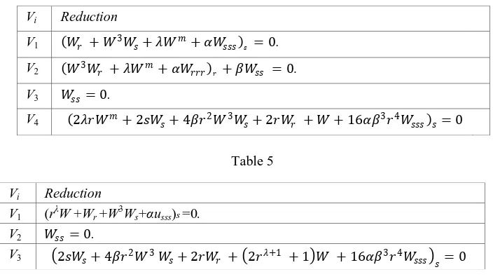
The reductions of one-dimensional sub algebras of equations (5.1) and (5.2, 5.3) are given in Table 4 ,Table 5 and Table 6.

Table 4

Table 5

[Vi,Vj] V1 V2 V3 V4

V1 0 0 0 V3

V2 0 0 0 −2βV1

V3 0 0 0 0

V4 V3 2βV1 0 0

[Vi,Vj] V1 V2 V3

V1 0 0 V2

V2 0 0 0

V3 V2 0 0

Vi Reduction

V1 𝑊𝑟 + 𝑊3𝑊𝑠+ 𝜆𝑊𝑚+ 𝛼𝑊𝑠𝑠𝑠 𝑠 = 0.

V2 𝑊3𝑊𝑟 + 𝜆𝑊𝑚+ 𝛼𝑊𝑟𝑟𝑟 𝑟 + 𝛽𝑊𝑠𝑠 = 0.

V3 𝑊𝑠𝑠= 0.

V4 2𝜆𝑟𝑊𝑚+ 2𝑠𝑊_𝑠+ 4𝛽𝑟2𝑊3𝑊_𝑠+ 2𝑟𝑊_𝑟 + 𝑊 + 16𝛼𝛽3𝑟4𝑊_{𝑠𝑠𝑠 𝑠}= 0

Vi Reduction

V1 (rλW +Wr +W3Ws+αusss)s =0. V2 𝑊𝑠𝑠= 0.

ISSN: 2231-5373

http://www.ijmttjournal.org

Page 66

Table 6

The reductions of two-dimensional sub algebras of equations (5.1) and (5.2,5.3) are given in Table 7 and Table 8.

Table 7 Algebra Reduction

[V1,V2]=0 (H3H′+λHm+αH′′′)′ =0. [V2,V3]=0 H′′ =0.

[V3,V4]=0 H′ =L(ρ). Table 8 Algebra Reduction [V1,V2]=0 H′ =G1(ρ) [V2,V3] H′ =G2(ρ)

6. Conclusions

• In this paper a (2+1)-dimensional KdV equation with variable coefficient 𝑢_𝑡+ 𝑢3_𝑢

𝑥+ 𝛼𝑢𝑥𝑥𝑥 𝑥+ 𝛽𝑢𝑦𝑦 = 0, 𝛼, 𝛽 ∈ 𝑅+is subjected to Lie’s classical

method

• Equation (1.4) admits a five-dimensional symmetry group.

• It is established that the symmetry generators form a closed Lie algebra.

• Classification of symmetry algebra of (1.4) into one- and two-dimensional subalgebras is carried out.

• Systematic reduction to (1+1)-dimensional PDE and then to ODEs are

performed using one-dimensional and two-dimensional Abelian and solvable nonAbelian subalgebras.

• A solution of (1.4) containg two arbitrary functions of t is determined by reduction to a linear partial differential equation.

References

[1] Ahmad, A., Ashfaque H. Bokhari., Kara, A.H., Zaman, F.D Symmetry classifications and reductions of some classes of (2+1)-nonlinear heat equation, J. Math. Anal. Appl., 339: 175-181 (2008).

[2] Bluman, G. W. and Kumei, S., Symmetries and Differential Equations, Springer-Verlag, New York, 1989. Liu Z. and Yang C.,The application of bifurcation method to a higher-order KdV equation, J. Math. Anal. Appl., 275: 1-12 (2002).

[3] Miura, R.M., Korteweg-de Vries equations and generalizations. A remarkable explicit nonlinear transformation, I.Math. Phys. 9: 1202-1204 (1968).

[4] Olver, P. J., Applications of Lie Groups to differential equations, Graduate Texts in Mathematics, 107, Springer-Verlag, New York, 1986.

[5] Senthilkumaran, M., Pandiaraja, D. and Mayil Vaganan, B. New Exact explicit Solutions of the Generalized KdV Equations 2008 Appl. Math. comp. 202 693-699

[6] Whitham, G. B., Linear and Nonlinear Waves, Wiley, New York, 1974. Vi Reduction

V1 𝑟𝜆𝑊𝑚_{+ 𝑊}

𝑟 + 𝑊3𝑊𝑠+ 𝛼𝑢𝑠𝑠𝑠 _𝑠 = 0.

V2 𝑊𝑠𝑠= 0.

V3 2𝑠𝑊𝑠+ 4𝛽𝑟2𝑊 3_𝑊

𝑠+ 2𝑟𝑊𝑟+ 2𝑟𝜆+1𝑊

𝑚_{+ 𝑊 + 16𝛼𝛽}3_𝑟4𝑊