Scalable Approximations for Generalized Linear Problems
Murat A. Erdogdu [email protected]
Department of Computer Science Department of Statistical Sciences University of Toronto
Toronto, ON M5S 3G3, Canada
Mohsen Bayati [email protected]
Graduate School of Business Stanford University
Stanford, CA 94305, USA
Lee H. Dicker [email protected]
Department of Statistics and Biostatistics Rutgers University
Piscataway, NJ 08854, USA
Editor:Qiang Liu
Abstract
In stochastic optimization, the population risk is generally approximated by the empirical risk which is in turn minimized by an iterative algorithm. However, in the large-scale setting, empirical risk minimization may be computationally restrictive. In this paper, we design an efficient algorithm to approximate the population risk minimizer in generalized linear problems such as binary classification with surrogate losses and generalized linear regression models. We focus on large-scale problems where the iterative minimization of the empirical risk is computationally intractable, i.e., the number of observations n is much larger than the dimension of the parameter p (n p 1). We show that under random sub-Gaussian design, the true minimizer of the population risk is approximately proportional to the corresponding ordinary least squares (OLS) estimator. Using this relation, we design an algorithm that achieves the same accuracy as the empirical risk minimizer through iterations that attain up to a quadratic convergence rate, and that are computationally cheaper than any batch optimization algorithm by at least a factor ofO(p). We provide theoretical guarantees for our algorithm, and analyze the convergence behavior in terms of data dimensions. Finally, we demonstrate the performance of our algorithm on well-known classification and regression problems, through extensive numerical studies on large-scale datasets, and show that it achieves the highest performance compared to several other widely used optimization algorithms.
Keywords: Generalized Linear Problems, Stochastic optimization, Subsampling, Dimen-sion reduction in optimization.
1. Introduction
We consider the following stochastic optimization problem
minimize
β∈Rp R(β) :=E
Ψ (hx, βi)−yhx, βi
, (1)
c
where Ψ : R → R is a non-linear function, y ∈ Y ⊂ R denotes the response variable,
x ∈ X ⊂ Rp denotes the predictor (or covariate), and the expectation is over the joint
distribution of (y, x). The above minimization is called a generalized linear problem in its canonical representation, and it is commonly encountered in statistical learning. Celebrated examples include binary classification with smooth surrogate losses (Buja et al., 2005; Reid and Williamson, 2010), and generalized linear models (GLMs) such as Poisson regression, logistic regression, ordinary least squares, multinomial regression with many applications involving graphical models (Nelder and Baker, 1972; McCullagh and Nelder, 1989; Wain-wright and Jordan, 2008; Koller and Friedman, 2009). These methods play a crucial role in numerous machine learning and statistics problems, and they provide a miscellaneous framework for many regression and classification tasks.
The exact minimization of the stochastic optimization problem (1) requires the knowl-edge of the underlying distribution of the variables (y, x). In practice, however, the joint distribution of the pair is not available; therefore, after observingnindependent data points (yi, xi), the standard approach is to minimize the following surrogate of (1), often referred to as empirical risk approximation
minimize
β∈Rp Rb(β) :=
1
n n
X
i=1
Ψ (hxi, βi)−yihxi, βi. (2)
In the case of GLMs, the empirical risk minimization given in (2) is equivalent to the maximum likelihood estimation (MLE), whereas in the case of binary classification, it is generally referred to as surrogate loss minimization. Due to the non-linear structure of the optimization task given in (2), minimizing the empirical risk requires iterative methods. The first-order approximation of the non-linear risk yields the gradient descent algorithm, which attains a (local) linear convergence rate under certain conditions withO(np) per-iteration cost. Although its convergence rate is slow compared to that of the second-order methods, its modest per-iteration cost makes it practical for large-scale problems. Regardless of the problem formulation, the most commonly used optimization method for computing the MLE is the Newton-Raphson method, which may be viewed as a reweighted least squares algorithm (McCullagh and Nelder, 1989; Buja et al., 2005). This method uses a second-order approximation to benefit from the curvature of the log-likelihood and achieves locally quadratic convergence. A drawback of this approach is its excessive per-iteration cost of O(np2). To remedy this, Hessian-free Krylov sub-space based methods such as conjugate gradient can be used, but the resulting direction is imprecise (Hestenes and Stiefel, 1952; Paige and Saunders, 1975; Martens, 2010). In the regime n p, another popular optimization technique is the class of Quasi-Newton methods (Bishop, 1995; Nesterov, 2004), which can attain a per-iteration cost of O(np), and the convergence rate is locally super-linear; a well-known member of this class of methods is the BFGS algorithm (Broyden, 1970; Fletcher, 1970; Goldfarb, 1970; Shanno, 1970).
certain random predictor (design) models,
βpop∝βols. (3)
For logistic regression with Gaussian design (which is equivalent to Fisher’s discriminant analysis), (3) was noted by Fisher in the 1930s (Fisher, 1936); a more general formulation for models with Gaussian design is given in Brillinger (1982). The relationship (3) suggests that if the constant of proportionality is known, then βpop can be estimated by computing the OLS estimator, which may be substantially simpler than minimizing the empirical risk. In fact, in some applications like binary classification, it may not be necessary to find the constant of proportionality in (3). Our work in this paper builds on this idea.
Our contributions can be summarized as follows.
1. We show thatβpopis approximately proportional toβols in the random design setting, regardless of the covariate (predictor) distribution. That is, we prove
β
pop−c
Ψ×βols
∞.c
kβpopk∞ √
p ,
for some cΨ ∈R which depends on the non-linearity Ψ. We note that above rate is
the relative decay, and it is obtained under the assumption that E[hx, βpopi2] . c2.
Our generalization uses zero-bias transformations (Goldstein and Reinert, 1997). We also show that the relation (3) still holds under certain types of regularization.
2. We design a computationally efficient estimator for βpop by first estimating the OLS coefficients, and then estimating the proportionality constant cΨ via line search. We refer to the resulting estimator as the Scaled Least Squares (SLS) estimator and denote it by ˆβsls. After estimating the OLS coefficients, the second step of our algorithm in-volves finding a root of a real valued function; this can be accomplished using iterative methods with up to a quadratic convergence rate and only O(n) per-iteration cost. This is computationally cheaper than the classical batch methods such as gradient descent by at least a factor of O(p).
3. For random design with sub-Gaussian predictors and bounded Ψ(2), we show that
ˆ
βsls−βpop
∞.
kβpopk∞ √
p +
r
p n.
This bound characterizes the performance of the proposed estimator in terms of data dimensions, and justifies the use of the algorithm in the large-scale setting where
n p 1. We also provide theoretical guarantees when subsampling is utilized in the algorithm for further efficiency.
5. We propose a scalable optimization method for converting one generalized linear prob-lem to another by exploiting the proportionality relation (3). The proposed algorithm requires onlyO(n) computations per each iteration, with no additional one-time cost. We further discuss the canonicalization of the square loss, which may be of indepen-dent interest for non-convex optimization.
6. We empirically study the statistical and computational performance of ˆβsls, and com-pare it to that of the empirical risk minimizer (using several well-known implementa-tions), on a variety of large-scale datasets.
The rest of the paper is organized as follows: Section 1.1 surveys the related work and Section 2 introduces the required background and the notation. In Section 3, we provide the intuition behind the relationship (3), which are based on exact calculations for the Gaussian design setting. In Section 4, we propose our algorithm and discuss its computational properties. Theoretical results are given in Section 5. In Section 6, we propose an algorithm to convert one GLM type to another. We discuss how a binary classification problem can be cast as a generalized linear problem in Section 7, and in Section 7.1 we propose a method to canonicalize the square loss. Section 8 provides a thorough comparison between the proposed algorithm and other existing methods. Finally, we conclude with a brief discussion in Section 9.
1.1. Related work
As mentioned in Section 1, the relationship (3) is well-known in several forms in statistics literature. Brillinger (1982) derived (3) for models with Gaussian predictors using Stein’s lemma. Li and Duan (1989) studied model misspecification problems in statistics and derived (3) when the predictor distribution has linear conditional means (this is a slight generalization of Gaussian predictors). The relation (3) has led to various techniques for dimension reduction (Li, 1991; Li and Dong, 2009), and more recently, it has been studied by Plan and Vershynin (2016); Thrampoulidis et al. (2015) in the context of compressed sensing. It has been shown that the standard lasso estimator may be very effective when used in models where the relationship between the expected response and the signal is nonlinear, and the predictors (i.e. the design or sensing matrix) are Gaussian. A common theme for all of this previous work is that it focuses solely on settings where (3) holds exactly and the predictors (covariates) are Gaussian (or, in the case of Li and Duan (1989), very nearly Gaussian).
The proportionality relation is solely based on Stein’s lemma and its variants. There are recent studies using Stein’s lemma in various machine learning and optimization tasks such as second-order optimization (Erdogdu, 2015, 2016, 2017), Bayesian inference (Liu and Wang, 2016), measuring sample quality and model evaluation tasks (Gorham and Mackey, 2015; Liu et al., 2016).
2. Preliminaries and Notation
We assume a random design setting, where the observed data consists ofnrandom iid pairs (y1, x1), (y2, x2),. . ., (yn, xn);yi ∈ Y ⊂Ris the response variable andxi = (xi1,· · ·, xip)T ∈
X ⊂ Rp is the vector of predictors or covariates. We focus on problems where the
mini-mization (1) is desirable, but we allow model misspecification, and do not need to assume that (yi, xi) are actually drawn from a particular parametric model. In other words, the joint distribution of (yi, xi) can be arbitrary.
βpop= argmin
β∈Rp E
Ψ(hxi, βi)−yihxi, βi
. (4)
While we make no assumptions on Ψ beyond smoothness, note that when the optimiza-tion problem is GLM, and Ψ is the cumulant generating funcoptimiza-tion for yi | xi, then the
problem reduces to the standard GLM with canonical link and regression parametersβpop
(McCullagh and Nelder, 1989). Examples of GLMs in this form include logistic regression with Ψ(w) = log{1 +ew}, Poisson regression with Ψ(w) =ew, and linear regression (least
squares) with Ψ(w) =w2/2.
Our objective is to find a computationally efficient estimator for βpop. The alternative estimator forβpopproposed in this paper is related to the OLS coefficient vector, which is de-fined byβols:=E[xixTi ]−1E[xiyi]; the corresponding OLS estimator is ˆβols := (XTX)−1XTy,
whereX= (x1, . . . , xn)T is the n×pdesign matrix andy = (y1, . . . , yn)T ∈Rn.
Additionally, throughout the text we let [m] ={1,2, ..., m}, for positive integersm, and we denote the size of a set S by |S|. The m-th derivative of a function g : R → R is
denoted by g(m). For a vectoru∈
Rp and an×p matrixU, we let kukq and kUkq denote
the `q-vector and -operator norms, respectively. If S ⊆ [n], let US denote the |S| × p
matrix obtained from U by extracting the rows that are indexed by S. For a symmetric matrixM∈Rp×p,λ
max(M) andλmin(M) denote the maximum and minimum eigenvalues,
respectively, andρq(M) forq ∈ {1,2,∞}denotes the condition number ofMwith respect to
`q-norm. We denote byNp the p-variate normal distribution, and all expectations are over
all randomness inside the brackets. Finally, we use a . b and a≤ O(b) interchangeably, whichever is convenient (whereO(·) refers to the big O notation).
3. From OLS to the True Minimizer: Gaussian Case
To motivate our methodology, we assume in this section that the covariates are multivariate normal, as in Brillinger (1982). These distributional assumptions will be relaxed to a certain extent in Section 5.
Proposition 1 Assume that the covariates are multivariate normal with mean 0 and
co-variance matrix Σ, i.e. xi ∼Np(0,Σ). Then βpop can be written as
βpop=cΨ×βols, (5)
where cΨ∈R is the fixed point of the mapping
z→E h
Ψ(2)(hxi, βolsiz) i−1
Proof [of Proposition 1] The stationary point of the minimization problem in (4) satisfies the following normal equations,
E[yixi] =E h
xiΨ(1)(hxi, βi)
i
for i= 1,2, ..., p. (7)
Now, denote byφ(x|Σ) the multivariate normal density with mean 0 and covariance matrix
Σ. We recall the well-known property of Gaussian density dφ(x|Σ)/dx=−Σ−1xφ(x|Σ). Using this and the integration by parts on the right hand side of the above equation, we obtain for i= 1,2, ..., p
E h
xiΨ(1)(hxi, βi) i
= Z
xΨ(1)(hx, βi)φ(x|Σ) dx, (8) =Σβ EΨ(2)(hxi, βi)
| {z }
∈ R
,
which is basically the Stein’s lemma. Combining this with the normal equations (7) and multiplying both side withΣ−1, we obtain the desired result.
Proposition 1 and its proof provide the main intuition behind our proposed method. Observe that in our derivation, we only worked with the right hand side of the normal equations (7) which does not depend on the response variableyi. Therefore, the equivalence
will hold regardless of the joint distribution of (yi, xi). This is the main difference from the proof of Brillinger (1982) whereyi is assumed to follow a single index model. In Section 5,
where we extend the method to non-Gaussian predictors, the identity (8) is generalized via the zero-bias transformations from Goldstein and Reinert (1997).
3.1. Regularization
A version of Proposition 1 incorporating regularization — an important tool for datasets wherepis large relative tonor the predictors are highly collinear — is also possible, as out-lined briefly in this section. We focus on`2-regularization (ridge regression) in this section; some connections with lasso (`1-regularization) are discussed in Section 5 and Corollary 6.
For λ≥0, define the `2-regularized empirical risk minimizer, βλpop= argmin
β∈Rp E
[Ψ(hxi, βi)−yihxi, βi] + λ 2 kβk
2
2 (9)
and the corresponding `2-regularized OLS coefficients βλols = ExixTi
+λI−1
E[xiyi] (so βpop=β0pop andβols=β0ols). The same argument as above implies that
βpopλ =cΨ×βγols, where γ =λcΨ. (10)
Algorithm 1 SLS: Scaled Least Squares Estimator
Input: Data (yi, xi)ni=1
Step 1. Compute the least squares estimator: βˆols and yˆ=Xβˆols.
For a sub-sampling based OLS estimator, letS ⊂[n] be a random subset and take ˆβols= |Sn|(XTSXS)−1XTy.
Step 2. Solve the following equation for c∈R: 1 = nc Pn
i=1Ψ(2)(cyˆi).
Use Newton’s root-finding method: Initialize c;
Repeat until convergence:
c←c− c
1 n
Pn
i=1Ψ(2)(cyˆi)−1 1
n
Pn
i=1
Ψ(2)(cyiˆ) +cyiˆΨ(3)(cyiˆ) . Output: ˆβsls=c×βˆols.
4. SLS: Scaled Least Squares Estimator
Motivated by the results in the previous section, we design a computationally efficient algorithm that approximates the stochastic optimization problem (1) that is as simple as solving the least squares problem; it is described in Algorithm 1. The algorithm has two basic steps. First, we estimate the OLS coefficients, and then in the second step we estimate the proportionality constant via a simple root-finding algorithm.
There are numerous fast optimization methods to solve the least squares problem, and even a superficial review of these could go beyond the page limits of this paper. We empha-size that this step (finding the OLS estimator) does not have to be iterative and it is the main computational cost of the proposed algorithm. We suggest using a sub-sampling based esti-mator forβols, where we only use a subset of the observations to estimate the covariance ma-trix. LetS⊂[n] be a random sub-sample and denote byXS the sub-matrix formed by the rows ofXinS. Then the sub-sampled OLS estimator is given as ˆβols = |S1|XTSXS−1 1
nX Ty.
Properties of sub-sampling and sketching based estimators have been well-studied (Ver-shynin, 2010; Dhillon et al., 2013; Erdogdu and Montanari, 2015; Pilanci and Wainwright, 2015; Roosta-Khorasani and Mahoney, 2016a,b). For sub-Gaussian covariates, it suffices to use a sub-sample size of O(plog(p)) (Vershynin, 2010). Hence, this step requires a single time computational cost of O |S|p2+p3+np
≈ O pmax{p2log(p), n}
. For other ap-proaches, we refer reader to Rokhlin and Tygert (2008); Drineas et al. (2011); Dhillon et al. (2013); Erdogdu and Montanari (2015) and the references therein.
0 20 40 60
4 5 6
log10(n)
Time
(
s
e
c
)
Method SLS MLE
SLS vs MLE : Computation
0.0 0.3 0.6 0.9 1.2
4 5 6
log10(n)
|
β
^−
β
|2
Method SLS MLE
SLS vs MLE : Accuracy
1e−04 1e−03 1e−02 1e−01 1e+00
4 5 6
log10(n)
lo
g10
(|
β
^ −
β
|2
) MethodSLS
MLE
SLS vs MLE : Log−Accuracy
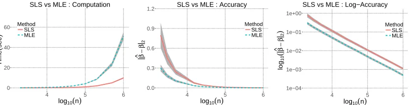
Figure 1: Logistic regression with iid standard Gaussian design. The left plot shows the computa-tional cost (time) for finding the MLE and SLS asngrows andp= 200. The middle and the right plots depict the accuracy of the estimators in standard and log scales, respectively. In the regime where the MLE is expensive to compute, the SLS is found much more rapidly and has the same accuracy. R’s built-in functions are used to find the MLE.
Correct initialization of the scaling constantcdepends on the optimization problem. For example, in the case of GLM problems, assuming that the GLM is a good approximation to the true conditional distribution, by the law of total variance and basic properties of GLMs, we have
Var (yi) =E[Var (yi |xi)] + Var (E[yi|xi])≈c−Ψ1+ Var Ψ(1)(hxi, βi)
. (11)
It follows that the initialization c = 2/Var (yi) is reasonable as long as we have c−Ψ1 ≈
E[Var (yi|xi)] not much smaller than Var Ψ(1)(hxi, βi). Our experiments show that SLS
is very robust to initialization.
In Figure 1, we compare the performance of our SLS estimator to that of the MLE in a GLM optimization problem, when both are used to analyze synthetic data generated from a logistic regression model under general Gaussian design with randomly generated covariance matrix. The left plot shows the computational cost of obtaining both estimators as n increases for fixed p = 200. The middle and the right plots show the accuracy of the estimators where the latter is in log-scale. In the regime n p 1 — where the MLE is hard to compute — the MLE and the SLS achieve the same accuracy, yet SLS has significantly smaller computation time. We refer the reader to Section 5 for theoretical results characterizing the finite sample behavior of the SLS.
5. Theoretical Results
In this section, we use the zero-bias transformations (Goldstein and Reinert, 1997) to gen-eralize the equivalence relation given in the previous section to the settings where the covariates are non-Gaussian.
Definition 2 Let z be a random variable with mean 0 and varianceσ2. Then, there exists a random variablez∗ that satisfiesE[zf(z)] =σ2E[f(1)(z∗)], for all differentiable functions
f. The distribution of z∗ is said to be the z-zero-bias distribution.
transformation is itself (i.e. the normal distribution is a fixed point of the operation mapping the distribution ofz to that ofz∗ – which is basically Stein’s lemma).
To provide some intuition behind the usefulness of the zero-bias transformation, we refer back to the proof of Proposition 1. For simplicity, assume that the covariate vectorxi has
iid entries with mean 0, and variance 1. Then the zero-bias transformation applied to the
j-th normal equation in (7) yields
E[yixij] =E h
xijΨ(1) xijβj+ Σk6=jxikβk
i
| {z }
j-th normal equation
=βjE h
Ψ(2) x∗ijβj+ Σk6=jxikβik
i
| {z }
Zero-bias transformation
. (12)
The distribution of x∗ij is the xij-zero-bias distribution and is entirely determined by the distribution of xij; general properties of x∗ij can be found, for example, in Chen et al. (2010). If β is well spread, it turns out that taken together, with j = 1, . . . , p, the far right-hand side in (12) behaves similar to the right side of (8), with Σ = I; that is, the behavior is similar to the Gaussian case, where the proportionality relationship given in Proposition 1 holds. This argument leads to an approximate proportionality relationship for problems with non-Gaussian predictors, which, when carried out rigorously, yields the following result.
Theorem 3 Suppose that the whitened covariates wi = Σ−1/2
xi are independent random
vectors with mean 0, covarianceI, and sub-Gaussian normκx. Furthermore,wi’s have
con-stant first and second conditional moments, i.e.,∀j∈[p]andβ˜=Σ1/2βpop,
E[wij
Σk6=jβ˜kwik] andE[w2ij
Σk6=jβkwik˜ ]are deterministic, and the function Ψ(2) is Lipschitz continuous with
constant k. Then, for cΨ= 1/EΨ(2)(hxi, βpopi)
, we have
1
cΨ
×βpop−βols
∞
≤ηkΣ1/2βpopk∞kβpopk∞, where η = 8kκ3xρ∞. (13)
Theorem 3 is proved in Section 10 of the Appendix. It implies that the population parame-ters βols and βpop are approximately equivalent up to a scaling factor, with arelative error bound of O(kΣ1/2βpopk
∞). For the above analysis to provide a decreasing bound in the
dimension p, one needs a tractability assumption on either one of the terms in the error bound. The most common way to achieve this is to introduce a structure on the inner prod-uct between x and βpop, e.g.
E[hx, βpopi2]1/2 =O √p suffices to get a decay in (13). We
emphasize that it is common practice to standardize the response and the features before training any model; therefore this preliminary procedure can provide the required order and consequently the desired decay inp.
Below, we discuss two commonly encountered settings in the literature as two corollaries.
Corollary 4 Let the assumptions of Theorem 3 hold. If we further assume that the
covari-ates xi are supported on a ball of radius r, and Σ1/2 is diagonally dominant, we have
1
cΨ
×βpop−βols
∞
≤ηkβ
popk2 ∞
√
p , where η= 16krκ
3 x
√
ρ2ρ∞. (14)
matrix appropriately, and then using the proposed estimator. This assumption is common in many fields, yet can appear in different forms. For example in the machine learning litera-ture, the standard convention (the same setting in Corollary 4) is to assume thatkxik2≤r,
and that kβpopk2 = O √p
(Kalai and Sastry, 2009; Shalev-Shwartz et al., 2009; Kakade et al., 2011), or the inner product is supported on an interval |hx, βpopi| ≤b almost surely (Alquier and Biau, 2013), where the latter is a more strict assumption. In the compressed sensing and other areas in statistics, a similar assumption is imposed on the covariance matrixExxT= ˜Σ/pwhich provides us withE[kxk22] =O(1) (Donoho et al., 2009; Bayati
and Montanari, 2012; Bayati et al., 2013; Su and Candes, 2016).
On the other hand, the standard convention in the dimension reduction techniques is to assume that the covariates have norm of order √p, i.e. E[kxk2] = O
√
p, and the coefficients have norm of order 1, i.e. kβk2 = τ = O(1) (Duan and Li, 1991; Hall and Li, 1993; Hristache et al., 2001). This setting again yields that the inner product between those two vectors are tractable and provides us with a decay in the latter term, i.e. kβpopk∞=O 1/√p. In this setting, Theorem 3 yields the following corollary.
Corollary 5 Let the assumptions of Theorem 3 hold. If we further assume that βpop is r-well-spread in the sense that forkβpopk2=τ, we haveτ /kβpopk∞=r√pfor somer ≤1,
1
cΨ ×β
pop−βols
∞
≤ηkβ
popk
∞
√
p , where η= 8kκ
3
xρ∞(τ /r)kΣ1/2k∞. (15)
In the above bound, the decay is in fact 1/p, but we chose to state the relative decay. We emphasize that both settings in Corollaries 4 and 5 are equivalent and both assumptions lead a tractable inner producthx, βpopi. The constants κx,ρk are invariant to the scalings considered in both settings.
The assumption that βpop is well-spread can be relaxed with minor modifications. For example, if we have a sparse coefficient vector, where supp(βpop) = {j; βjpop 6= 0} is the support set of βpop, then Corollary 5 holds with p replaced by the size of the support set.
The assumptions on the conditional moments are the relaxed versions of assumptions that are commonly encountered in dimension reduction techniques. For example, sliced inverse regression methods assume that the first conditional moment Exhx, βi
is linear in x for all β (Li and Duan, 1989; Li, 1991), which is satisfied by elliptically distributed random vectors. An important case that is not covered by these methods is the independent coordinate case, i.e., when the whitened covariates have independent, but not necessarily identical entries. This is made possible by introducing additional approximation error (i.e. suboptimality due to non-Gaussian design). We refer reader to Li and Dong (2009), for a good review of dimension reduction techniques and their corresponding assumptions. We also highlight that our moment assumptions can be relaxed further, at the expense of introducing some additional complexity into the results.
An interesting consequence of Theorem 3 and the corollaries following the theorem is that whenever an entry ofβpop is zero, the corresponding entry ofβols has to be small, and conversely. For λ≥0, define the lasso coefficients
βλlasso = argmin
β∈Rp
1 2E
Corollary 6 Let supp(β) denote the support of β, i.e., the set {i∈ [p] : βi 6= 0}. Given
kc1
Ψβ
pop−βolsk
∞≤δ, and for any λ≥δ, if E[xi] = 0 and ExixTi
=I, we have
supp(βlasso)⊂supp(βpop).
Further, if λand βpop also satisfy that ∀j ∈supp(βpop), |βjpop|> cΨ(λ+δ), then we have
supp(βlasso) = supp(βpop).
We note that δ above can be obtained using Theorem 3 or its corollaries. So far in this section, we have only discussed properties of the population parameters, such as βpop and
βols. In the remainder of this section, we turn our attention to the results on the estimators that are the main focus of this paper; these results ultimately build on our earlier results, i.e. Theorem 3. We will be considering the setting in Corollary 5 in the rest of this section, i.e.,kxk2 =O √p
andkβpopk
2 =O(1). Results presented below can be easily generalized
to the setting in Corollary 4 as well.
In order to precisely describe the performance of ˆβsls, we first need bounds on the OLS estimator. The OLS estimator has been studied extensively in the literature; however, for our purposes, we find it convenient to derive a new bound on its accuracy. While we have not seen this exact bound elsewhere, it is very similar to Theorem 5 of Dhillon et al. (2013).
Proposition 7 Assume that E[xi] = 0, ExixTi
= Σ, and that Σ−1/2xi and yi are
sub-Gaussian with norms κ and γ, respectively. For λmin denoting the smallest eigenvalue of
Σ, and|S|> ηp,
ˆ
βols−βols
2
≤ηλmin−1/2
r p
|S|, (17)
with probability at least 1−3e−p, where η depends only on γ and κ.
Proposition 7 is proved in Section 10. Our main result on the performance of ˆβsls is given next.
Theorem 8 Let the assumptions of Theorem 3, Corollary 5, and Proposition 7 hold.
Fur-ther assume that Ψ(2)
≤b and for some ¯c and the function f(z) =zE
Ψ(2)(hx, βolsiz)
satisfiesf(¯c)>1 +, and the derivative off in the interval [0,¯c]does not change sign, i.e.,
its absolute value is lower bounded by υ > 0. Then, for n and |S| sufficiently large, with
probability at least 1−4e−p, we have
ˆ
βsls−βpop
∞≤η1
kβpopk∞ √
p +η2
r p
|S|, (18)
where the constants η1 and η2 are defined by
η1=ηk¯cρ∞(τ /r)kΣ1/2k∞ (19) η2=η¯c
λ−min1/2+kυ−1maxn(kΣ1/2βolsk2+ 1)kΣk2+b/k,¯co, (20)
Note that the convergence rate of the upper bound in (18) depends on the sum of the two terms, both of which are functions of the data dimensionsn and p. The first term on the right in (18) comes from Theorem 3 and Corollary 5, which bounds the discrepancy betweencΨ×βols andβpop. This term is small when pis large, and it does not depend on
the number of observations n. If n and p grow together, then p has to grow at a smaller rate to achieve convergence. We note that the actual decay of this term is O(1/p) (since
kβpopk∞=O 1/√p
), but we state the relative decay which isO 1/√p .
The second term in the upper bound (18) comes from estimating βols and cΨ. This term is increasing in p, which reflects the fact that estimating βpop is more challenging when p is large. As expected, this term is decreasing in n and |S|, i.e. larger sample size yields better estimates. When the full OLS solution is used (|S| = n), the second term becomes O(pp/n), which suggests that the sample size should be at least of order p for good performance. We note that in the case of Gaussian covariates,√n-consistency follows since we don not have a bias term.
In certain loss functions, the uniform boundedness assumption on Ψ(2)may be too strict. However, this assumption can be removed by making an additional assumption that the covariates have bounded support. This yields the same decay rateOpp/n
in the second term. However, if one needs to preserve the sub-Gaussian assumption on the covariates, then the above analysis – when carried out without the uniform bound assumption on Ψ(2) – yields the following result. We note that we still require the uniform Lipschitz assumption but one can always utilize the local Lipschitz properties of the function Ψ(2).
Theorem 9 Let the assumptions of Theorem 3, Corollary 5, and Proposition 7 hold with
E[kΣ−1/2xk2] = ˜µ
√
p. Further assume that supβ:kβ−Σ1/2βolsk 2≤1kΨ
(2)(hxi, βi)k
ψ2 ≤ κg and
for some ¯c and the function f(z) = zEΨ(2)(hx, βolsiz) satisfies f(¯c) > 1 +, and the
derivative of f in the interval [0,¯c] does not change sign, i.e., its absolute value is lower
bounded by υ >0. Then, for n and|S|sufficiently large, with probability at least 1−5e−p, we have
ˆ
βsls−βpop
∞≤η1
kβpopk∞ √
p +η2
r p
min{n/log(n),|S|}, (21)
where the constants η1 and η2 are defined by
η1=ηk¯cρ∞(τ /r)kΣ1/2k∞ (22) η2=η¯c
λ1/2min+υ−1kβolsk∞max{(κg+k/µ˜), k¯cκx}
, (23)
and η >0 is a constant depending on κx and γ.
We observe that this time when the full OLS solution is used (|S|=n), the second term becomesO(pplog(n)/n), which is worse than the rate given in Theorem 8 by a logarithmic factor. In this setting, we require that n/log(n) should be at least of order p for good performance. Also, note that there is a theoretical threshold for the sub-sampling size|S|, namely O(n/log(n)), beyond which further sub-sampling provides no improvement.
5.1. Convergence in `2-norm
In the sequel, we assume that the full OLS solution is used (|S|=n). Using Proposition 7 and Lemma 16, we can show that the `2-distance between the estimator ˆβsls and the pop-ulation parametercΨβols converges to 0 with rate
√
nwhenp is fixed. It is straightforward to see that under Gaussian design, this leads to consistency in `2-norm with convergence
rate √n. However, the quantity cΨβols is in general different from βpop under general sub-Gaussian design; thus, in such cases consistency cannot be achieved in the classical setting wherep is fixed (see i.e. Claim 1 in Chen and Banerjee (2017)). In such a scenario, Theo-rem 3 can be used to obtain an upper bound on the suboptimality resulting from general sub-Gaussian design.
In order to talk about consistency when n, p → ∞ under `2-norm, a normalization by
one of the growing dimensions is required, see e.g. Bayati and Montanari (2012); Bayati et al. (2013). Hence, in this regime, we focus on the quantity √1
pkβˆ
sls−βpopk
2 under the
assumptions of Corollary 4 with Σ = I. Since we have √n-convergence of our estimator to the population parametercΨβols, consistency reduces to showing that the suboptimality term √1
p
cΨβols−βpop
2 converges to 0. This term can be controlled with additional sparsity-type structural assumptions on the problem. Below, we discuss two scenarios that may lead to such a setting.
Sparsity. Assume thatβpophassnon-zero terms, i.e.,kβpopk0=s. Following the same proof technique of Theorem 3, we can show that
1
√
p
cΨβ
ols−βpop
2 ≤C
rs
pkβ
popk
∞, (24)
for some constant C > 0. As long as the non-sparsity level satisfies s = O(p), we can attain consistency in `2-norm. The rate of convergence will be determined by the growing rates of n, p(n) and s(n). For example, to attain √n-convergence, one needs s = O(1) and p=O(n), but milder growth conditions can still lead to consistency at the expense of slower convergence.
Normality. Similarly, one can assume that a subset of features with size s follow a non-Gaussian distribution, and the remaining p−sfeatures are normally distributed. The same argument above can also provides consistency in`2-norm – again in this case and the convergence rate will be determined by the ratio ps/p.
5.2. Verifying the key assumptions
The assumption on f(z) = zEΨ(2)(hx, βolsi, z) appears in both theorems and depends
both on the function Ψ and the underlying covariate distribution. Therefore, in order to verify this assumption rigorously, one needs to know the distribution of the covariates which is not always available. However, a straightforward way to verify this assumption is to use the sample mean estimate ˆf(z) = zn1Pn
i=1Ψ(2)(hxi,βˆolsiz) using the dataset at hand to
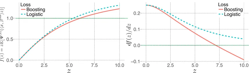
estimate f(z). In Figure 2, we use this technique to verify that our assumptions are valid for two commonly used loss functions, namely, boosting and logistic regression when the covariates are normally distributedx ∼N(0,1pI) and kβolsk2 =
√
0.0 0.5 1.0
0.0 2.5 5.0 7.5 10.0
Loss Boosting Logistic
−0.1 0.0 0.1 0.2
0.0 2.5 5.0 7.5 10.0
Loss Boosting Logistic
Figure 2: We demonstrate how to validate our assumption onf(z) =zEΨ(2)(hx, βolsiz)
on two commonly used loss functions. Left plot shows f(z), whereas right plots shows its derivative. In these plots, covariates are generated fromx∼N(0,I/p), andkβolsk
2 =
√
p/4.
The assumption on f(z) can be verified by a more rigorous treatment. For simplicity, we again consider the compressed sensing setting where we assume x ∼N(0,1pI), and this time we let kβpopk2 = cΨ
βols
2 ≈
√
p. In order to obtain a scaling constant cΨ ≤ 20,
assume that we have βols
2 =
√
p/20.
Boosting loss: In this case, we have Ψ(z) =z/2 +p1 +z2/4 which yields
Ψ(2)(z) = 1 4(1 +z
2/4)−3/2 and Ψ(4)(z) = 3
64
5z2(1 +z2/4)−2−4
(1 +z2/4)5/2 . (25)
We notice that both of these functions are even, i.e., Ψ(2)(z) = Ψ(2)(−z), and Ψ(4)(z) = Ψ(4)(−z). We use the local convexity for z≥0 aroundz= 2, and obtain Ψ(2)(z)≥a−bz
where a = Ψ(2)(2)−2Ψ(3)(2) and b = −Ψ(3)(2). For W ∼ N(0,1) and φ denoting the standard normal density, we write
f(z) =zE h
Ψ(2)(hx, βolsiz) i
=zE h
Ψ(2)(W z/20) i
, (26)
=2z
Z ∞
0
Ψ(2)(wz/20)φ(w)dw≥2z
Z 20a/bz
0
(a−bwz/20)φ(w)dw,
= 2z
aΦ(20a/bz)−a
2−
bz
20√2π(1−e
−200a2/b2z2)
.
Using the above bound, we observe that for ¯c= 6 and δ=.23, we havef(¯c)>1 +δ. Next, we verify the derivative condition on f, that is, f(1) does not change sign in the interval [0,¯c]. By the Stein’s lemma, we write
f(1)(z) =E h
Ψ(2)(W z/20)i+ (z/20)2E h
Ψ(4)(W z/20)i. (27)
Using the previous inequalities together with the above expression, we have
f(1)(z)≥E h
Ψ(2)(W z/20)i− 9
100 Ψ
(4)
(28)
≥2
aΦ(20a/bz)−a
2 −
bz
20√2π(1−e
−200a2/b2z2)
− 27
which verifies the derivative assumption onf(z).
Logistic regression: In this case, we have Ψ(z) = log(1 +ez) which yields
Ψ(2)(z) = e
z
(1 +ez)2 and Ψ
(4)(z) = ez(1−4ez+e2z)
(1 +ez)4 . (29)
As before, both Ψ(2) and Ψ(4) are even functions. Again, appealing to the local convexity properties, for z ≥ 0 around z = 2.5, we obtain Ψ(2)(z) ≥ a−bz where a = Ψ(2)(2.5)−
2.5Ψ(3)(2.5) and b=−Ψ(3)(2.5). Using (26), we obtain
f(z)≥2z
aΦ(20a/bz)−a
2 −
bz
20√2π(1−e
−200a2/b2z2
)
. (30)
Using the above bound, we see that for ¯c= 6, andδ =.22 we havef(¯c)>1 +δ. For the derivative bound, we again use (27), and obtain that for z∈[0,¯c],
f(1)(z)≥EhΨ(2)(W z/20)i− 9
100 Ψ
(4)
≥E
h
Ψ(2)(W z/20)i− 9
800 ≥0.19, (31) which verifies the assumption.
6. Converting One GLM to Another
In this section, we assume that one has already obtained a set of coefficients by minimizing a certain GLM loss, but wants to minimize another GLM loss using the same dataset. It is often the case that a practitioner would like to change the loss function (or equivalently the model) based on its performance. However, when the dataset is large, training a new model from scratch is extremely time consuming. In the following, we will use the proportionality relation to transition between different loss functions.
Assume that a practitioner fitted a GLM using the loss function (or cumulant generating function) Ψ1, but they would like to train a new model based on the second loss function
Ψ2. Instead of minimizing the new loss based on Ψ2, one can exploit the proportionality
relation and obtain the coefficients for the new GLM problem. Denote by βpop1 and βpop2
the GLM coefficients corresponding to the loss functions Ψ1 and Ψ2, respectively. Using
the results in the previous sections, we have
1
cΨ1
β1pop= 1
cΨ2
β2pop=βols,
for the normal case, that is, both coefficients are proportional to the OLS coefficients which does not depend on the loss function. Therefore, these coefficients β1pop and β2pop are also proportional to each other and we can write
β2pop= cΨ2
cΨ1
β1pop:=ρ β1pop, (32) where the proportionality constant between two different GLM types turns out to be the ratio betweencΨ1 and cΨ2, i.e. ρ=cΨ2/cΨ1. Using the definition ofcΨ2, we write
1 =cΨ2 E
h
Ψ(2)2 (hx, β2popi) i
,
=cΨ1ρ E
h
Algorithm 2 Conversion from one GLM to another
Input: Data (yi, xi)ni=1, and ˆβ1glm
Step 1. Compute yˆ=Xβˆ1glm, and κ= n1Pn
i=1Ψ (2) 1 (ˆyi). Step 2. Solve the following equation for ρ∈R: κ= nρPn
i=1Ψ (2) 2 (ˆyiρ)
Use Newton’s root-finding method: Initialize ρ= 1;
Repeat until convergence:
ρ←ρ− ρ
1 n
Pn
i=1Ψ (2)
2 (ρyiˆ)−κ 1
n
Pn
i=1
n
Ψ(2)2 (ρyˆi) +ρyˆiΨ(3)2 (ρyˆi)
o.
Output: ˆβglm2 =ρ×βˆ1glm.
Dividing the both sides bycΨ1 and using the equalityc
−1 Ψ1 =E
h
Ψ(2)1 (hx, β1popi)i, we obtain
E h
Ψ(2)1 (hx, β1popi)i=ρ E h
Ψ(2)2 (hx, β1popiρ)i.
The above equation only involves β1pop as the coefficients (which is assumed to be already known/obtained by the practitioner). Therefore, if we solve it for the ratio ρ, we can estimate β2pop by simply using the proportionality relation given in (32).
The procedure described above is summarized as Algorithm 2. We emphasize that this procedure does not require the computation of the OLS estimator which was the main cost of SLS, and it only requires a per-iteration cost of O(n). In other words, conversion from one GLM type to another is easier compared to obtaining the GLM coefficients from scratch.
7. Binary Classification with Proper Scoring Rules
In this section, we assume that for i∈[n], the response is binary yi ∈ {0,1}. The binary
classification problem can be described by the following minimization of an empirical risk
minimize
β∈Rp 1
n n
X
i=1
`(yi;q(hxi, βi)), (33)
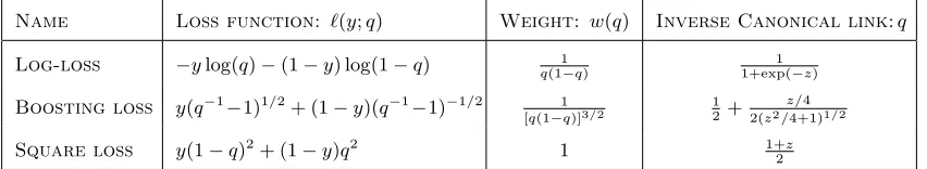
where ` and q are referred to as the loss and the link functions, respectively. There are various loss functions that are used in practice. Examples include log-loss, boosting loss, square loss etc (See Table 1). As before, we constrain our analysis on the canonical links. The concept of canonical links for binary classification is introduced by Buja et al. (2005), and it is quite similar to the generalized linear problems.
For any given loss function, we define the partial losses`k(·) =`(y=k;·) fork∈ {0,1}.
Since we have a binary response variable, we can write any loss in the following format
`(y;q) =y`1(q) + (1−y)`0(q),
Table 1: Common loss functions and their inverse canonical links
Name Loss function: `(y;q) Weight: w(q) Inverse Canonical link:q
Log-loss −ylog(q)−(1−y) log(1−q) q(1−1q) 1+exp(−1 z)
Boosting loss y(q−1−1)1/2+ (1−y)(q−1−1)−1/2 [q(1−1q)]3/2
1 2 +
z/4 2(z2/4+1)1/2
Square loss y(1−q)2+ (1−y)q2 1 1+2z
The above formulation is of the form of a generalized linear problem. Before moving forward, we recall the concept of proper scoring in binary classification, which is sometimes referred to as Fisher consistency.
Definition 10 (Proper scoring rules) Assume that y ∼ Bernoulli(η). If the expected
loss E[`(y, q)] is minimized by q = η for all η ∈ (0,1), we call the loss function a proper
scoring rule.
The following theorem by Schervish (1989) provides a methodology for constructing a loss function for the proper scoring rules.
Theorem 11 (Schervish (1989)) Let w(dt) be a positive measure on (0,1) that is finite
on interval(,1−) ∀ >0. Then the following defines a proper scoring rule
`1(q) = Z 1
q
(1−t)w(dt), and`0(q) = Z q
0
tw(dt).
The measure w(dt) uniquely defines the loss function (generally referred to as the weight function, since all losses can be written as weighted average of cost weighted misclassification error (Buja et al., 2005; Reid and Williamson, 2010)). Examples of weight functions is given in Table 1. The above theorem has many interesting interpretations; one that is most useful to us is that `(1)0 (q) =qw(q).
The notion of canonical links for proper scoring rules are introduced by Buja et al. (2005), which corresponds to the notion of matching loss (Helmbold et al., 1999; Reid and Williamson, 2010). The derivation of canonical links stems from the Hessian of the above minimization, which remedies two potential problems: non-convexity and asymptotic variance inflation. It turns out that by setting w(q)q(1) as constant, one can remedy both problems (Buja et al., 2005). We will skip the derivation and, without loss of generality, assume that the canonical link-loss pair satisfies w(q)q(1) = 1. Note that any loss function has a natural canonical link. The following Theorem summarizes this concept.
Theorem 12 (Buja et al. (2005)) For proper scoring rules with w > 0, there exists a canonical link function which is unique up to addition and multiplication by constants. Conversely, any link function is canonical for a unique proper scoring rule.
The canonical link for a given loss function can be explicitly derived from the equation
link for proper scoring rules, we write the normal equations dβdE[`(y, q(hx, βi))] = 0 as
E h
xq(1)(hx, βi)`(1)0 (q(hx, βi)) i
=E
h
yxq(1)(hx, βi)
`(1)0 (q(hx, βi))−`(1)1 (q(hx, βi)) i
,
=⇒ Ehxq(1)(hx, βi)q(hx, βi)w(q(hx, βi))i=E h
yxq(1)(hx, βi)w(q(hx, βi))i,
=⇒ E[xq(hx, βi)] =E[yx],
=⇒ ΣβE
h
q(1)(hx, βi)i=E[yx].
The last equation provides us with the analog of the proportionality relation we observed in generalized linear problems. In this case, we observe that the proportionality constant becomes 1/Eq(1)(hx, βi). Therefore, our algorithm can be used to obtain a fast training
procedure for the binary classification problems under canonical links as well.
7.1. Canonicalization of the Square Loss
Consider a minimization problem of the following form
minimize
β
1
n n
X
i=1
[yi−f(hxi, βi)]2. (34)
The above problem is commonly encountered in many machine learning tasks – specifically, in the context of neural networks, the functionf is called the activation function. Here, we consider a toy example to demonstrate how our methodology can be useful in a minimization problem of the above form.
We first use Taylor series expansion around a point θ (which should be close tohx, βi), in order to approximate the function f(z) with a linear function around f(θ). We write
min
β E
(y−f(hx, βi))2≈min
β E
f(hx, βi)2−2yhx, βif0(θ). (35) The above approximation yields
Ψ(z) = f(z)
2
2f0(θ), (36)
and the proportionality relation given in previous sections would hold for the approximation, which will be accurate when the activation function is smooth around the user-specified point θ. This method can be used to derive proportionality relations for GLMs with non-canonical links (conditional on the link being nice), and also may be of interest in non-convex optimization, e.g., reliable initialization.
8. Experiments
8.1. Numerical Analysis of Convergence
0.00 0.01 0.02 0.03 0.04 0.05
25 50 75 100
p
|
β
pop
−
cΨ
β
ols|
∞
|
β
pop
|∞
Convergence of Population Parameters
0 25 50 75
4 5 6
log10(n)
Time
(
s
e
c
)
Method SLS MLE
SLS vs MLE : Computation
0.001 0.010 0.100 1.000
4 5 6
log10(n)
|
β
^ −
β
|2
Method SLS MLE
SLS vs MLE : Log−Accuracy
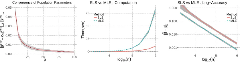
Figure 3: Logistic regression with iid Bernoulli±1 design. The left plot shows the relative error between the population parameters. The middle plot shows the computational cost (time) for finding the MLE and SLS as n grows andp = 200. The right plot depict the accuracy of the estimators in log scale. In the regime where the MLE is expensive to compute, the SLS is found much more rapidly and has the same accuracy. R’s built-in functions are used to find the MLE.
parameters with respect to the dimension. In this experiment, we estimate the relative error
βpop−cΨβols
∞/kβ
popk
∞ using a Monte-Carlo simulation. The dimension takes values
fromp∈ {5,10,15, ...,100}, and for each fixedp, we choose the sample sizen(p) =Kpwhere
K = 10,000. βpop = (1,1, ...,1)/√p is fixed throughout this experiment. Covariates are generated from a Bernoulli distribution P(xij =±1) = 0.5, and the response is generated
from the logistic model. We estimateβols using coordinatewise average of the ordinary least squares estimator over the whole dataset. The scaling constant is estimated by the inverse of n1 Pn
i=1Ψ(2)(hxi, βpopi). We repeat this experiment 100 times for eachp, and the results
are reported in left plot in Figure 3. We observe that the relative error decreases with increasing dimension.
The second experiment demonstrates the effect of sample size. In this experiment, we fix p = 200, and the sample size varies n ∈ 103 × {2,3,5,15,25,50,100,200,500,1000}. Covariates are again generated from Bernoulli distribution P(xij =±1) = 0.5, and the
response is generated from the logistic model. Maximum likelihood estimator is obtained through R’s built-in function glm. We report the computation time of these estimators as well as their estimation error in the middle and the right plots in Figure 3, respectively. We observe that MLE performs consistently better in terms of test error, yet it is significantly expensive to compute when ngets larger. In the large-scale regime, the difference between the achieved test errors becomes negligible as seen in the right plot. This is the regime that SLS provides significant advantage. We also emphasize that MLE and SLS has the same convergence rate as can be observed in the right plot.
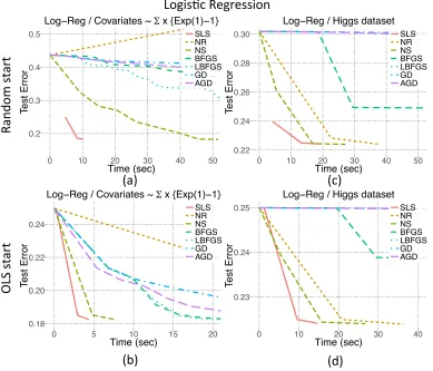
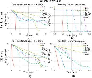
8.2. Comparisons With Other Optimization Methods
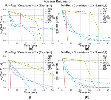
This section contains the results of a variety of numerical studies, which show that the Scaled Least Squares estimator reaches its minimum achievable test error substantially faster than commonly used batch algorithms for finding the MLE. Both logistic and Poisson regression models (two types of GLMs) are utilized in our analyses, which are based on several synthetic and real datasets.
Ran
do
m
s
tar
t
O
LS
s
tar
t
Logis0c Regression
(a)
(b)
(c)
(d)
0.20.3 0.4 0.5
0 10 20 30 40 50
Time (sec)
Test Error
SLS NR NS BFGS LBFGS GD AGD
Log−Reg / Covariates ~ Σ x {Exp(1)−1}
0.22 0.24 0.26 0.28 0.30
0 10 20 30 40 50
Time (sec)
Test Error
SLS NR NS BFGS LBFGS GD AGD Log−Reg / Higgs dataset
0.23 0.24 0.25
0 10 20 30 40
Time (sec)
Test Error
SLS NR NS BFGS LBFGS GD AGD Log−Reg / Higgs dataset
0.18 0.20 0.22 0.24
0 5 10 15 20
Time (sec)
Test Error
SLS NR NS BFGS LBFGS GD AGD Log−Reg / Covariates ~ Σ x {Exp(1)−1}
Figure 4: We compared the performance of SLS to that of MLE for the logistic regres-sion problem on several datasets. MLE optimization is solved by various optimization algorithms. SLS is represented with red straight line. The details are provided in Table 2.
1. Newton-Raphson (NR) achieves locally quadratic convergence by scaling the gra-dient by the inverse of the Hessian evaluated at the current iterate. Computing the Hessian has a per-iteration cost ofO np2, which makes it impractical for large-scale datasets.
2. Newton-Stein (NS)is a recently proposed second-order batch algorithm specifically designed for GLMs (Erdogdu, 2015, 2016). The algorithm uses Stein’s lemma and sub-sampling to efficiently estimate the Hessian with a cost of O(np) per-iteration, achieving near quadratic rates.
Ran
do
m
s
tar
t
O
LS
s
tar
t
Poisson Regression
(e)
(g)
(f)
(h)
0.5 1.0 1.5 2.0
0 10 20 30 40
Time (sec)
log(T
est Error)
SLS NR NS BFGS LBFGS GD AGD Poi−Reg / Covariates ~ Σ x Ber(±1) 0.5
1.0 1.5 2.0 2.5
0 10 20 30 40
Time (sec)
log(T
est Error)
SLS NR NS BFGS LBFGS GD AGD Poi−Reg / Covariates ~ Σ x Ber(±1)
0 5 10 15
0.0 2.5 5.0 7.5 10.0
Time (sec)
log(T
est Error)
SLS NR NS BFGS LBFGS GD AGD Poi−Reg / Covertype dataset 0.5
1.0 1.5 2.0
0.0 2.5 5.0 7.5 10.0
Time (sec)
log(T
est Error)
SLS NR NS BFGS LBFGS GD AGD Poi−Reg / Covertype dataset
Figure 5: We compared the performance of SLS to that of MLE for the Poisson regres-sion problem on several datasets. MLE optimization is solved by various optimization algorithms. SLS is represented with red straight line. Details are given in Table 2.
4. Limited memory BFGS (LBFGS)is a variant of BFGS, which uses only the recent iterates and gradients to approximate the Hessian, providing significant improvement in terms of memory usage. LBFGS has many variants; we use the formulation given in Bishop (1995).
5. Gradient descent (GD) takes a step in the opposite direction of the gradient, evaluated at the current iterate. Its performance strongly depends on the condition number of the design matrix. Under certain assumptions, the convergence is linear withO(np) per-iteration cost.
6. Accelerated gradient descent (AGD) is a modified version of gradient descent with an additional “momentum” term (Nesterov, 1983). Its per iteration cost isO(np) and its performance strongly depends on the smoothness of the objective function.
Table 2: Details of the experiments shown in Figures 4 and 5 with simulated and real datasets HIGGS (Baldi et al., 2014), and Covertype (Blackard and Dean, 1999)
Model Logistic regression Poisson regression
Dataset Σ×{Exp(1)-1} Higgs Σ×Ber(±1) Covertype Size n= 6.0×10⁵,p= 300 n= 1.1×10⁷,p= 29 n= 6.0×10⁵,p= 300 n= 5.8×10⁵,p= 53
Initial Rnd Ols Rnd Ols Rnd Ols Rnd Ols
Plot (a) (b) (c) (d) (e) (f) (g) (h)
Method↓ Time in seconds / number of iterations (to reach min test error)
Sls 8.34/4 2.94/3 13.18/3 9.57/3 5.42/5 3.96/5 2.71/6 1.66/20
Nr 301.06/6 82.57/3 37.77/3 36.37/3 170.28/5 130.1/4 16.7/8 32.48/18
Ns 51.69/8 7.8/3 27.11/4 26.69/4 32.71/5 36.82/4 21.17/10 282.1/216
Bfgs 148.43/31 24.79/8 660.92/68 701.9/68 67.24/29 72.42/26 5.12/7 22.74/59
Lbfgs 125.33/39 24.61/8 6368.1/651 6946.1/670 224.6/106 357.1/88 10.01/14 10.05/17
Gd 669/138 134.91/25 100871/10101 141736/13808 1711/513 1364/374 14.35/25 33.58/87
Agd 218.1/61 35.97/12 2405.5/251 2879.69/277 103.3/51 102.74/40 11.28/15 11.95/25
Recall that the proposed Algorithm 1 is composed of two steps; the first finds an estimate of the OLS coefficients. This up-front computation is not needed for any of the MLE algorithms described above. On the other hand, each of the MLE algorithms requires some initial value for β, but no such initialization is needed to find the OLS estimator in Algorithm 1. This raises the question of how the MLE algorithms should be initialized, in order to compare them fairly with the proposed method. We consider two scenarios in our experiments: first, we use the OLS estimator computed for Algorithm 1 to initialize the MLE algorithms; second, we use a random initial value.
On each dataset, the main criterion for assessing the performance of the estimators is how rapidly the minimum test error is achieved. The test error is measured as the mean squared error of the estimated mean using the current parameters at each iteration on a test dataset, which is a randomly selected (and set-aside) 10% portion of the entire dataset. As noted previously, the MLE is more accurate for smalln (see Figure 1). However, in the regime considered here (np1), the MLE and the SLS perform very similarly in terms of their error rates; for instance, on the Higgs dataset, the SLS and MLE have test error rates of 22.40% and 22.38%, respectively. For each dataset, the minimum achievable test error is set to be the maximum of the final test errors, where the maximum is taken over all of the estimation methods. Let Σ(1) and Σ(2) be two randomly generated covariance matrices. The datasets we analyzed were: (i) a synthetic dataset generated from a logistic regression model with iid{exponential(1)−1}predictors scaled byΣ(1); (ii) the Higgs dataset (logistic regression) Baldi et al. (2014); (iii) a synthetic dataset generated from a Poisson regression model with iid binary(±1) predictors scaled by Σ(2); (iv) the Covertype dataset (Poisson regression) Blackard and Dean (1999).
9. Discussion
In this paper, we showed that the true minimizer of a generalized linear problem and the OLS estimator are approximately proportional under the general random design setting. Using this relation, we proposed a computationally efficient algorithm for large-scale problems that achieves the same accuracy as the empirical risk minimizer by first estimating the OLS coefficients and then estimating the proportionality constant through iterations that can attain quadratic or cubic convergence rate, with onlyO(n) per-iteration cost.
We briefly mentioned that the proportionality between the coefficients holds even when there is regularization in Section 3.1. Further pursuing this idea may be interesting for large-scale problems where regularization is crucial. Another interesting line of research is to find similar proportionality relations between the parameters in other large-scale opti-mization problems such as support vector machines. Such relations may reduce the problem complexity significantly.
10. Proof of Main Results
In this section, we provide the details and the proofs of our technical results. For conve-nience, we briefly state the following definitions.
Definition 13 (Sub-Gaussian) For a given constant κ, a random variable x∈R is said
to be sub-Gaussian if it satisfies supm≥1m
−1/2
E[|x|m]1/m ≤κ. Smallest such κ is the
sub-Gaussian norm of x and it is denoted by kxkψ2. Similarly, a random vector y ∈ Rp is a
sub-Gaussian vector if there exists a constant κ0 such that supv∈Sp−1khy, vikψ2 ≤κ0.
Definition 14 (Sub-exponential) For a given constant κ, a random variable x ∈ R is
called sub-exponential if it satisfies supm≥1m−1E[|x|m] 1/m ≤
κ. Smallest such κ is the
sub-exponential norm of x and it is denoted by kxkψ1. Similarly, a random vector y ∈Rp
is a sub-exponential vector if there exists a constantκ0 such that supv∈Sp−1khy, vikψ1 ≤κ0. The proof of Theorem 3 is given next.
Proof [of Theorem 3] For simplicity, we denote the whitened covariate by w = Σ−1/2x. Since w is sub-Gaussian with norm κ, itsj-th entry wj has bounded third moment. That
is,
κ= sup
kuk2=1
khu, wikψ
2 ≥ kwjkψ2 = sup
m≥1
m−1/2E[|wj|m]1/m≥
1
√
3E
|wj|3
1/3
, (37)
where in the first step, we usedu=ej, thej-th standard basis vector. Hence, we obtain a bound on the third moment, i.e,
max
j E
|wj|3
≤33/2κ3. (38)
Using the normal equations, we write
E[yx] =E h
xΨ(1)(hx, βi) i
=Σ1/2E h
wΨ(1)(hw,Σ1/2βi) i
, (39)
=Σ1/2E h
where we defined ˜β=Σ1/2β. By multiplying both sides withΣ−1, we obtain
βols =Σ−1/2E h
wΨ(1)(hw,β˜i)i. (40) Now we define the partial sumsW−i=Pj6=iβjwj˜ =hβ, w˜ i −βi˜wi. We will focus on the i-th entry of the above expectation given in (40). Denoting the zero biased transformation of wi conditioned on W−i bywi∗, we have
E h
wiΨ(1)(hw,β˜i)
i =E
h E
h
wiΨ(1)
˜
βiwi+W−i
W−i
ii
, (41)
= ˜βiE h
Ψ(2)( ˜βiw∗i +W−i)
i
,
= ˜βiE h
Ψ(2)( ˜βi(w∗i −wi) +hw,β˜i)
i
,
where in the second step, we used the assumption on conditional moments. Let D be a diagonal matrix with diagonal entries Dii = E
h
Ψ(2)( ˜βi(w∗i −wi) +hw,β˜i)
i
. Using (40)
together with (41), we obtain the equality
βols =Σ−1/2Dβ˜=Σ−1/2DΣ1/2β. (42) Now, using the Lipschitz continuity assumption of the variance function, we have
E
h
Ψ(2)( ˜βi(w∗i −wi) +hw,β˜i) i
−E
h
Ψ(2)(hw,β˜i) i
≤k|
˜
βi|E[|w∗i −wi|]. (43)
In the following, we will use the properties of zero-biased transformations. Consider the quantity
r= supE
|wi∗−wi|
W−i
E|wi|3W−i
(44)
wherew∗i haswi-zero biased distribution (conditioned onW−i) and the supremum is taken
with respect to all random variables with mean 0, standard deviation 1 and finite third moment, and w∗i is achieving the minimal `1 coupling to wi conditioned on W−i. It is
shown in Goldstein (2007) that the above bound holds for r = 1.5 for the unconditional zero-bias transformations. Here, we take a similar approach to show that the same bound holds for the conditional case as well. By using the triangle inequality, we have
E|wi∗−wi|
W−i
≤E
|w∗i| W−i
+E|wi|
W−i
(45)
≤1
2E
|wi|3
W−i
+E|wi|3
W−i
1/3
.
SinceE|wi|2W−i
is constant, it is equal toE|wi|2= 1. This yields that the second term
in the last line is upper bounded by E|wi|3
W−i
. Consequently, by taking expectations over both hand sides we obtain that
E[|w∗i −wi|]≤1.5E
|wi|3
Then the right hand side of (43) can be upper bounded by
k|β˜i|E[|w∗i −wi|]≤rkmax i
n
|β˜i|E|wi|3
o
≤8kκ3kΣ1/2βk∞, (47)
where in the second step we used the bound on the third moment given in (38). The last inequality provides us with the following result,
max i
Dii−
1 cΨ
≤8kκ3kΣ1/2βk∞. (48)
Finally, combining this with (40) and (42), we obtain
βols− 1
cΨ β ∞ =
Σ−1/2DΣ1/2β− 1
cΨ β ∞ (49) =
Σ−1/2
D− 1
cΨ I
Σ1/2β
∞ , ≤max i
Dii− 1
cΨ Σ 1/2 ∞ Σ −1/2
∞kβk∞,
≤8kκ3ρ∞kΣ1/2k∞kβpopk2∞,
which completes the proof.
Proof [of Corollary 4] Due to diagonal dominance property, we have
kΣ1/2k∞= max i p X j=1 Σ 1/2 ij
≤2 maxi Σ
1/2
ii ≤2kΣk 1/2
2 . (50)
Since we have kxk2 ≤r, we write
r2 ≥Ehkxk22i= Tr (Σ)≥pkΣk2/ρ2. (51)
Combining this with the previous inequality we obtain
kΣ1/2k∞≤2r
p
ρ2/p. (52)
Finally, the result follows from using the last bound in Theorem 3.
Proof[of Corollary 5] The result directly follows from using ther-well-spreadness assump-tion in Theorem 3.
Proof [of Proposition 7] For convenience, we denote the whitened covariates by wi = Σ−1/2xi. We haveE[wi] = 0,EwiwiT
=I, and kwikψ
2 ≤κ. Also denote the sub-sampled covariance matrix withΣb = |S1|
P
i∈SxixTi , and its whitened version asΣe = |S1| P
i∈SwiwiT.
Further, define ˆζ = n1Pn
i=1wiyi and ζ =E[wy]. Then, we have
ˆ
βols =Σb
−1
For now, we work on the event that Σb is invertible. We will see that this event holds with very high probability. We write
Σ
1/2( ˆβols−βols) 2=
Σ
1/2
b
Σ−1Σ1/2ζˆ−Σ−1/2ζ
2, (53)
= Σe
−1n ˆ
ζ−ζ+I−Σ−1/2ΣΣb −1/2
ζo
2,
≤
Σe
−1
2
n ˆ
ζ−ζ
2+
I−Σe
2kζk2
o
,
where we used the triangle inequality and the properties of the operator norm. For the first term on the right hand side of (53), we write
Σe
−1 2 =
1
λmin(Σe)
≤ 1
1−δ,
where we assumed that such a δ > 0 exists. In fact, when δ < 0.5, we obtain a bound of 2 on the right hand side, which also justifies the invertibility assumption of Σb. By Corollary 5.50 of Vershynin (2010) and the following remark, we have with probability at least 1−2 exp{−p},
Σe −I
2
≤c
r p
|S|,
wherec is a constant depending only onκ. When|S|>4c2p, we obtain
λmin(Σe)−1
≤
Σe −I
2≤0.5,
where the first inequality follows from the Lipschitz property of the eigenvalues.
Next, we bound the difference between ˆζ and its expectation ζ. We write the bounds on the sub-exponential norm
kwykψ
1 = sup
kvk2=1
sup
m≥1
m−1E[|hv, wiy|m]1/m, (54)
≤ sup
kvk2=1
sup
m≥1
m−1E|hv, wi|2m1/2mE|y|2m1/2m,
≤ sup
kvk2=1
sup
m≥1
m−1/2E|hv, wi|2m1/2msup
m≥1
m−1/2E|y|2m1/2m, ≤2kwkψ
2kykψ2 = 2γκ.
Hence, we have maxikwiyi−E[wiyi]kψ1 ≤4γκ. Further, let ej denote the j-th standard basis, and notice that each entry ofwis also sub-Gaussian with norm upper bounded byκ, i.e.,
κ=kwkψ
2 = sup
kuk2=1
khu, wikψ
Also, we can write
2γκ≥ kwykψ
1 = sup
kuk2=1
sup
m≥1
m−1E[|hu, wiy|m]1/m, (55)
≥ sup
kuk2=1
E[|hu, wiy|],
≥ sup
kuk2=1
E[hu, wiy] = sup
kuk2=1
hu, ζi=kζk2,
where in the last step, we used the fact that dual norm of `2 norm is itself.
Next, we apply Lemma 17 to ˆζ−ζ, and obtain with probability at least 1−exp{−p}
ˆ
ζ−ζ
2 ≤cγκ
r
p n,
whenever n > c2pfor an absolute constant c.
Combining the above results in (53), we obtain with probability at least 1−3 exp{−p}
Σ
1/2( ˆβols−βols)
2 ≤2
c1γκ
r
p
n+c2γκ
r p
|S|
≤η
r p
|S| (56)
whereη depends only on κ and γ, and |S|> ηp. Finally, we write
ˆ
βols−βols
2≤λ −1/2 min
Σ
1/2( ˆβols−βols)
2,
≤ηλ−min1/2
r p
|S|,
with probability at least 1−3 exp{−p}, whenever |S|> ηp.
The following lemma – combined with the Proposition 7 – provides the necessary tools to prove Theorem 9.
Lemma 15 For a given function Ψ(2) that is Lipschitz continuous with constant k, we
define the function f : R×Rp → R as f(c, β) = c EΨ(2)(hx, βic), and its empirical
counterpart as
ˆ
f(c, β) =c 1 n
n
X
i=1
Ψ(2)(hxi, βic).
For the ball centered around βols with radius δ,
Bδ( ˜βols) = n
β :β−β˜ols
2 ≤δ
o
, with β˜ols = Σ1/2βols, assume that supβ∈Bδ( ˜βols)
Ψ(2)(hx, βi)
ψ2 ≤κg, and
Σ−1/2xi
ψ2 ≤κx. Further, for some