Mathematical modelling and simulation of the human circulation with emphasis on the venous system: application to the CCSVI condition

(1)

Mathematical modelling and simulation of the human

circulation with emphasis on the venous system:

application to the CCSVI condition

Lucas Omar M¨

uller

(2)

(3)

Doctoral thesis inEnvironmental Engineering, XXVI cycle

Department of Civil, Environmental and Mechanical Engineering, University of Trento Academic year 2014/2015

Supervisor: Prof. Eleuterio Francisco Toro

(4)

(5)

Abstract

Recent advances in medical science regarding the role of the venous system in the devel-opment of neurological conditions has renewed the attention of researchers in this district of the cardiovascular system. The main goal of this thesis is to perform a theoretical study of Chronic CerebroSpinal Venous Insufficiency (CCSVI), a venous pathology that has been as-sociated to Multiple Sclerosis. CCSVI is a condition in which main cerebral venous drainage pathways are obstructed. Its impact in cerebral hemodynamics and its connection to Multiple Sclerosis is subject of current debate in the medical community. In order to perform a credible study of the haemodynamical aspects of CCSVI, a sufficiently accurate mathematical model of the problem under investigation must be used. The venous system has not received the same attention as the arterial counterpart by the medical community. As a consequence, the mathematical modeling and numerical simulation of the venous system lies far behind that of the arterial system. The venous system is a low-pressure system, formed by very thin-walled vessels, if compared to arteries, that are likely to collapse under the action of gravitational or external forces. These properties set special requirements on the mathematical models and numerical schemes to be used. In this thesis we present a closed-loop multi-scale mathematical model of the cardiovascular system, where medium to large arteries and veins are represented as one-dimensional (1D) vessels, whereas the heart, the pulmonary circulation, capillary beds and intracranial pressure are modeled as lumped parameter models. A characteristic feature of our closed-loop model is the detailed description of head and neck veins. Due to the large inter-subject variability of the venous system, we perform a patient-specific characterization of major veins of the head and neck using MRI data collected in collaboration with the Magnetic Resonance Research Facility of the Wayne State University, Detroit (USA). Computational re-sults are carefully validated using published data for the arterial system and most regions of the venous system. For head and neck veins validation is carried out through a detailed comparison of simulation results against patient-specific Phase-Contrast MRI flow quantification data. Re-garding the development of novel numerical schemes, we construct high-order accurate, robust and efficient numerical schemes for 1D blood flow in elastic and viscoelastic vessels, as well as a solver for vessel networks. The solver is validated in the context of an in vitro network of vessels for which experimental and numerical results are available. After validation of both, the mathematical model and the numerical methodology, we use our theoretical tool to study the influence of different CCSVI patterns on cerebral hemodynamics. CCSVI patterns are defined by the medical literature as combinations of venous obstructions at different locations. Here we used two strategies. First, we take a venous configuration corresponding to a healthy control and explore the effect of different CCSVI patterns by modifying this network. Then, we char-acterize our venous network with the geometry of a real CCSVI patient and compare results with the ones obtained for the healthy control. The presented model provides a powerful tool to study still unresolved aspects of cerebral blood flow physiology, as well as several venous pathologies. Furthermore, it constitutes an ideal platform for improving currently used algo-rithms and for integrating fundamental physiological processes, such as detailed hemodynamics, regulatory mechanisms and transport of substances.

(6)

(7)

Acknowledgments

My first thought goes to my wife Wenddi. Her support and encouragement have been fundamental during this long-term project. I am proud and honored for having the opportunity to build our family together. I would also like to express my profound gratitude to my family. Without the many sacrifices made by my parents I could have never completed this long journey. I was extremely fortunate to have met Prof. Eleuterio F. Toro during my undergraduate studies. I am grateful for his guidance during these years and for the many opportunities that he has offered me. I hope to have fully absorbed his dedication to science and will always be grateful for this opportunity.

I would like to thank Prof. Carlos Par´es and his group at the University of M´alaga. My stay at their institute and the work carried out together was an essential initiation to the numerical solution of non-conservative hyperbolic systems. A thought goes also to Prof. Michael Dumbser. He was always available when I had doubts regarding the numerical methodology adopted in this thesis.

I am pleased to acknowledge Gino I. Montecinos for the time spent together during this PhD project. He has become a precious friend and his support as applied mathematician has been fundamental at many stages of my work. A thought goes also to Alfonso Caiazzo, his help in making the code developed during the completion of this thesis more readable and modular was fundamental.

An essential aspect of my PhD research project was the opportunity offered to me by Prof. E. M. Haacke (MR Research Facility, Wayne State University, Detroit, USA) to visit his research facility during two months in order to gather the MRI data used in this work. During my stay in Detroit I learned a lot about the anatomy of the venous system and became familiar with MRI imaging techniques. In this context I would also like to mention the support received from David Utriainen.

I would like to thank Prof. Zamboni and his team, for the many instructive visits to Ferrara and Bologna and their visits to Trento. These meetings were fundamental for two reasons: understanding the physiology of the venous system and finding motivation for the development of our work.

A special thank goes to Prof. Carmelo Anile, from the Institute of Neurosurgery of the Catholic University in Rome, for useful discussions on cerebral venous hemodynamics and his contribution to the extension of our mathematical model.

A thought goes to the International Society of Neurovascular Disease. At the beginning of this research project we took part to an annual meeting as spectators and with the time we were given the opportunity to actively participate. This fact shows that this society is truly interested in the insights that mathematics can give to their research.

I would also like to warmly thank Dr. Jordy Alastruey (King’s College and St Thomas’ Hospital, London, UK) for very helpful discussions that contributed to the development of my solver for blood flow in networks of vessels and for sharing with me his numerical results and experimental measurements. This information was essential for the validation of my work.

I conclude this section expressing my gratitude to the PhD School in Environmental Engi-neering at the Department of Civil, Environmental and Mechanical EngiEngi-neering of the Univer-sity of Trento, for the financial support of this PhD research project in terms of scholarships and allowances for participating to relevant conferences and schools.

(8)

(9)

Scientific production

Papers published or submitted during this PhD research project:

• L. O. Müller, G. I. Montecinos, and E. F. Toro. Some issues in modelling venous haemo-dynamics. In P. Garc´ıa-Navarro M. E. Vázquez-Cendón, A. Hidalgo and L. Cea, editors, Numerical Methods for Hyperbolic Equations: Theory and Applications. An international conference to honour Professor E. F. Toro, pages 347–354. Taylor & Francis Group, Boca Raton London New York Leiden, 2013.

• L. O. M¨uller, C. Par´es, and E. F. Toro. Well-balanced high-order numerical schemes for one-dimensional blood flow in vessels with varying mechanical properties. Journal of Computational Physics, 242:53 – 85, 2013.

• L. O. M¨uller and E. F. Toro. Well-balanced high-order solver for blood flow in net-works of vessels with variable properties. International Journal for Numerical Methods in Biomedical Engineering, 29:1388–1411, 2013.

• L. O. M¨uller and E. F. Toro. A global multiscale mathematical model for the human circulation with emphasis on the venous system. International Journal for Numerical Methods in Biomedical Engineering, pages n/a–n/a, 2014. In Press.

• G. Montecinos, L. M¨uller, and E. F. Toro. Hyperbolic reformulation of a 1D viscoelastic blood flow model and ADER finite volume schemes. Journal of Computational Physics, 2014. In Press.

• A. Caiazzo, G. Montecinos, L. O. M¨uller, E. M. Haacke, and E. F. Toro. Computational haemodynamics in stenotic internal jugular veins. Journal of Mathematical Biology. Sub-mitted for publication to the Journal of Mathematical Biology in May 2013.

• L. O. M¨uller and E. F. Toro. An enhanced closed-loop model for the study of cerebral venous blood flow. Submitted for publication to the Journal of Biomechanics in March 2014.

• L. O. M¨uller, E. F. Toro, and E. M. Haacke. A theoretical study of the CCSVI condition. Submitted for publiction to the Journal of the Royal Society Interface in March 2014.

(12)

(13)

List of Figures

2.1 Wave speed (2.11). Parameters: A0= 0.001m2,m= 10,n=−1.5,ρ= 1050_mkg3,

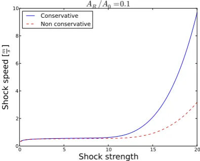
K= 5P a. . . 12 2.2 Elastic jump speeds obtained using the conservative and non-conservative

for-mulations. Parameters: A0= 0.001m2,m= 10,n=−1.5,ρ= 1050_mkg3,K= 5P a 12

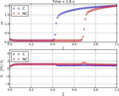
2.3 Giraffe jugular vein collapse test. Solution at output time t= 1.6s, during the transient phase. C: conservative formulation; NC: non-conservative formulation. . 13 2.4 Giraffe jugular vein collapse test. Solution at output timet= 40.0s,

correspond-ing to the steady solution. C: conservative formulation; NC: non-conservative formulation. . . 13 3.1 Graph of the functiong(A) (3.25) and four horizontal lines corresponding to four

different values of Γ such that (1) Γ > 1₂ρ_Aq¯

0

2

, (2) 0<Γ < 1₂ρ_Aq¯

0

2

, (3) Γ<0, (4) Γ = 1₂ρ_Aq¯

0

2

. . . 23 3.2 Case Γ> 1₂ρ_Aq¯

0

2

. (a) Graph of K =f. (b) Integral curve (continuous line) and critical states (dashed lines). This line separates the subcritical region (to the left) from the supercritical region (to the right). . . 24 3.3 Case 0< Γ< 1₂ρ_Aq¯

0

2

. (a) Graph of K =f. (b) Integral curve (continuous line) and critical states (dashed lines). . . 24 3.4 Case Γ<0. (a) Graph ofK=f. (b) Integral curve (continuous line) and critical

states (dashed lines). . . 25 3.5 Case Γ = 1₂ρ_Aq¯

0

2

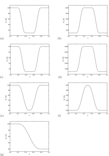
. (a) Graph of K =f. (b) Integral curve (continuous line) and critical states (dashed lines). . . 25 3.6 Case ¯q= 0. (a) Γ>0.(b) Γ>0. . . 26 3.7 Case ¯q= 0, Γ = 0. . . 26 3.8 K(x) for the presented steady state tests. (a) steady subcritical solution in Ω+_;

(b) steady subcritical solution in Ω−; (c) steady supercritical solution in Ω+_{; (d)}

steady supercritical solution in Ω−; (e) steady transcritical solution in Ω+_{; (f)}

steady transcritical solution in Ω−; (g) steady transcritical solution in Ω . . . 45 3.9 Steady tests for subcritical solutions (SUB-1 and SUB-2) and supercritical

so-lutions (SUP-1 and SUP-2) with smooth variation ofK. First and third-order results are shown in the left and right columns respectively. Quantities shown are non-dimensional cross-subsectional area (left vertical axis) and error with respect to the exact solution (right vertical axis). . . 46 3.10 Steady tests for transcritical solution in Ω− (TRA-1), in Ω+ _{(TRA-2) and in Ω}

(TRA-3) with smooth variation ofK. First and third-order results are shown in the left and right columns respectively. Quantities shown are non-dimensional cross-subsectional area (left vertical axis) and error with respect to the exact solution (right vertical axis). . . 47

(14)

3.11 Wave propagation test at t = 0.01s. Non-dimensional cross-subsectional area

α and velocity u for the first-order well-balanced scheme (a), the third-order well-balanced ADER scheme (b) and the third-order ADER scheme with non well-balanced WENO reconstruction (c). . . 48 3.12 Wave propagation test at t = 0.01s. Non-dimensional cross-subsectional area

α and velocity u for the first-order non well-balanced scheme (a) and the non well-balanced third-order ADER scheme (b). . . 49 3.13 Wave propagation test at t= 0.043s. Non-dimensional cross-subsectional area

α and velocity u for the first-order well-balanced scheme (a), the third-order well-balanced ADER scheme (b) and the third-order ADER scheme with non well-balanced WENO reconstruction (c). . . 50 3.14 Wave propagation test at t= 0.043s. Non-dimensional cross-subsectional area

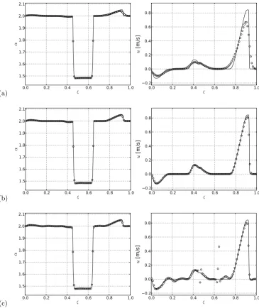
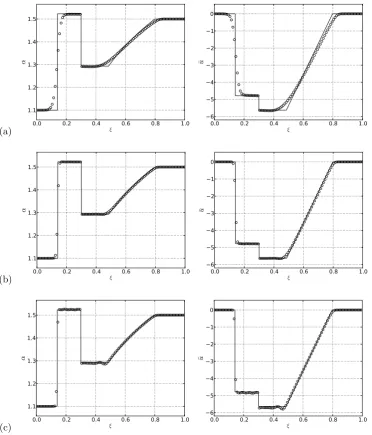
α and velocity u for the first-order non well-balanced scheme (a) and the non well-balanced third-order ADER scheme (b). . . 51 3.15 Riemann problem 1. Exact and numerical solutions for non-dimensional

cross-subsectional area and non-dimensional velocity. Results for the first-order well-balanced scheme (a), third-order well-well-balanced ADER scheme (b) and third-order ADER scheme with conventional WENO reconstruction (c). . . 52 3.16 Riemann problem 2. Exact and numerical solutions for non-dimensional

cross-subsectional area and non-dimensional velocity. Results for the first-order well-balanced scheme (a), third-order well-well-balanced ADER scheme (b) and third-order ADER scheme with conventional WENO reconstruction (c). . . 53 3.17 Riemann problem 3. Exact and numerical solutions for non-dimensional

cross-subsectional area and non-dimensional velocity. Results for the first-order well-balanced scheme (a), third-order well-well-balanced ADER scheme (b) and third-order ADER scheme with conventional WENO reconstruction (c). . . 54 3.18 Detail of region around the contact discontinuity for Riemann problem 2. Red

cir-cles represent the solutions obtained with the proposed third-order well-balanced ADER scheme, whereas black crosses show the solution obtained with a thrid-order numerical scheme that performs a conventional WENO reconstruction and uses a straight segment as integration path for computing fluctuations, instead of using the path specified in subsection 3.1.4. . . 55 3.19 Integration pathΨ(s) (3.117), on the (A, K) phase-plane, and integral curveγLD

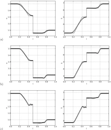
associated with the LD field for the case of fluid at rest. . . 63 3.20 Results for RP1 obtained using the first-order DOT solver with well-balanced

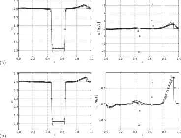
fluctuation (3.120) (top) and the first-order DOT solver with non well-balanced fluctuation (3.111) (bottom). Shown results are for non-dimensional cross-sectional area (left) and velocity (right) versus non-dimensional length. Note different ranges for velocity plots. . . 66 3.21 Exact solution and numerical results for RP2 regarding an (idealized) systolic

pressure and peak flow arriving to a portion of the thoracic aorta with discontinu-ous mechanical properties and external compression. Results obtained using the order DOT solver with well-balanced fluctuation (3.120) (top) and the first-order DOT solver with non well-balanced fluctuation (3.111) (bottom). Shown results are for non-dimensional cross-sectional area (left) and velocity (right) versus non-dimensional length. . . 67 3.22 Exact solution and numerical results for RP3, regarding an (idealized) Valsava

maneuver effect on an internal jugular vein with incompetent valve and dis-continuous mechanical properties. Results obtained using the first-order DOT solver with well-balanced fluctuation (3.120) (top) and the first-order DOT solver with non well-balanced fluctuation (3.111) (bottom). We show results for non-dimensional cross-sectional area (left) and velocity (right) versus non-non-dimensional length. . . 68 3.23 States across the stationary contact discontinuity, integral curveγLD(continuous

(15)

3.24 Error versus CPU time for second and fifth-order implementations of the ADER scheme. . . 72 3.25 Results for Riemann problems 1 to 3 using the third-order ADER scheme with

well-balanced fluctuation (3.120). Shown results are for non-dimensional cross-sectional area (left) and velocity (right) versus non-dimensional length. . . 73 3.26 Computed velocities at midpoint location versus time for all 37 vessels of the in

vitromodel fordead man test. Left frame shows results obtained using a WENO reconstruction in terms of pressure p and volumetric flow rate q; right frame shows results obtained using a WENO reconstruction for cross-sectional areaA

andq. . . 74 3.27 Performance of non well-balanced scheme for an unsteady problem. . . 75 3.28 Comparison of our numerical results in third-order mode against experimental

measurements and numerical results of [2]. . . 76 3.29 Comparison of numerical results obtained with the first-order scheme on refined

grids and with the higher order implementations on the original grid. Higher order schemes deliver a more accurate solution with less computational time, see table 3.10. . . 77 4.1 Arterial network composed of 85 arteries, taken from [101] (left). Detail of head

and neck arteries (right). Numbers refer to table 4.3, where geometrical and mechanical parameters for each vessel are reported. . . 81 4.2 Schematic representation of venous network (left). Detail of head and neck veins

(right). Numbers refer to table 4.8, where geometrical and mechanical parame-ters for each vessel are reported. . . 82 4.3 Lumped parameter model for heart and pulmonary circulation. RA, LA: right

and left atrium; RV, LV: right and left ventricles. T riV, P ulV, M itV, AorV: tricuspid, pulmonary, mitral and aortic valves. Pc and Pit are pericardium and

intra-thoracic pressures, respectively. In the present work both pressures are put equal to zero. . . 83 4.4 Lumped parameter network for a simple artery-vein connection. Arteries are

connected to veins via arterioles, capillaries and venules. For each compartment we specify complianceC, inductanceLand resistanceR. . . 83 4.5 Pressure vs non-dimensional cross-sectional area for tube law (4.16) withKA=

50000P a and P0 = 0mmHg (dotted line), for tube law (4.18) with KV =

0.011P a and P0 = 0mmHg (dashed line) and for tube law (4.18) with KV =

91.3P a and P0 = 5mmHg (continuous line). The top and middle rectangles

represent physiological pressure ranges for arteries and veins, respectively. . . 86 4.6 Single compartment used for lumped parameter models. The electric circuit

analog comprises a capacitor with capacitance C, a resistor with resistance R

and an inductor with inductanceL. . . 87 4.7 Error versus CPU time for second and fifth-order implementations of the ADER

scheme. . . 90 4.8 Exact solution and numerical results for the Riemann problem described in

sec-tion 4.1.3 regarding the effect of an (idealized) Valsava maneuver on an internal jugular vein with incompetent valve and discontinuous mechanical properties. Results for first and third order versions of the numerical schemes used in this work. Results shown for non-dimensional cross-sectional area (α=A/Aref) (left)

and velocity (right) versus non-dimensional length (ξ=x/L). . . 91 4.9 Lumped models A to C. The figure shows the indexes of feeding arteries, to the

left, and collecting veins, to the right. Parameters for resistances, inductors and capacitors are found in table 4.7. . . 97 4.10 Lumped models D to F. The figure shows the indexes of feeding arteries, to the

left, and collecting veins, to the right. Parameters for resistances, inductors and capacitors are found in table 4.7. . . 98 4.11 Lumped model G. The figure shows the indexes of feeding arteries, to the left,

(16)

4.12 MIP-TOF for a healthy patient (top) and patient-specific segmented geometry

and centerline extraction for head and neck veins (bottom). . . 100

4.13 Planes at which PC-MRI flow measures were acquired for neck veins at C2-C3, C5-C6 and C7-T1 levels (left) and for dural sinuses (right). The three acquisition planes along the neck allow to evaluate how flow rate increases as tributary veins merge the internal jugular veins, whereas the acquisition plane for dural sinues allows the evaluation of flow for the Superior Sagittal Sinus, the Straight Sinus and both Transverse Sinuses. . . 103

4.14 Computed pressures (top) and volumes (bottom) for the four cardiac chambers. RA: Right Atrium; RV: Right Ventricle; LA: Left Atrium; LV: Left Ventricle. . . 104

4.15 Blood flow distribution along the aorta and major leg arteries: computational resultsvsliterature data (average and standard deviation). Asc. Ao.: Ascending Aorta; Kidneys: sum of both Renal Arteries; Tho. Ao.: Thoracic Aorta; Abd. Ao.: Abdominal Aorta; Ext. Il. A.: External Iliac Artery; Fem. A.: Femoral Artery. Vessel numbers refer to table 4.3 and figure 4.1. References: a_Murgo_et al. [120]; bWolfet al. [176]; cZitnik et al. [186]; dChenget al. [51]; eItzchaket al. [86];fLewiset al. [100]. . . 105

4.16 Blood flow in head and neck arteries: computational results vs literature data (average and standard deviation). Brain: sum of average flow rate in both inter-nal carotid and vertebral arteries; ICA: Interinter-nal Carotid Artery; MCA: Middle Cerebral Artery; BA: Basilar Artery; VA: Vertebral Artery. Vessel numbers refer to table 4.3 and figure 4.1. References: a_{Stoquart-ElSankari}_{et al.} _[152];b_Stock et al. [151];c_Boorder_{et al.} _[33]. _{. . . 106}

4.17 Computed pressure and flow rate along the aorta. . . 107

4.18 Computed pressure and flow rate in the aorta and major leg arteries. . . 108

4.19 Computed pressure and flow rate in head and neck arteries. . . 109

4.20 Computed pressure values for arterioles, capillaries and venules for selected ele-ments of lumped compartele-ments E (top left), F (top right) and G (bottom row). p1 stands for arterioles, p2 for capillaries and pV enule for venules. Numbers correspond to the vessels that are connected to lumped compartment elements. . 110

4.21 Blood flow in selected systemic veins: computational results vs literature data (average and standard deviation). SVC: Superior Vena Cava; IVC: Inferior Vena Cava; AzG V.: Azygos Vein; SCV: Subclavian Vein. Vessel numbers refer to figure 4.2 and table 4.8. References: a _Be’eri _{et al.} _[24]; b _Cheng _{et al.} _[51]; c Nabeshimaet al. [123];d _{Fortune & Feustel [74]. . . 110}

4.22 Blood flow in head and neck veins: computational resultsvs MRI flow quantifi-cation data. SSS: Superior sagittal Sinus; StS: Straight Sinus; TS: Transverse Sinus; IJV: Internal Jugular Vein. Vessel numbers refer to figure 4.2 and table 4.8.111 4.23 Computed pressure and flow rate in selected systemic veins. . . 112

4.24 Computed pressure and flow rate in dural sinuses. PC-MRI flow quantification data is shown with symbols and dashed lines. . . 113

4.25 Computed pressure and flow rate in internal jugular veins. PC-MRI flow quan-tification data is shown with symbols and dashed lines. . . 114

4.26 Computed pressure and flow rate in internal jugular veins (cont. from figure 4.25). PC-MRI flow quantification data is shown with symbols and dashed lines. 115 4.27 Blood flow in neck veins for a venous network modified according to in table 4.11: computational results vs MRI flow quantification data. IJV: Internal Jugular Vein. Vessel numbers refer to figure 4.2 and table 4.11. . . 116

4.28 Computed pressure and flow rate in internal jugular veins for a venous network modified according to in table 4.11 . PC-MRI flow quantification data is shown with symbols and dashed lines. . . 117

(17)

4.30 Schematic representation of the closed-loop model presented in [117]. Major ar-teries and veins are described with a one-dimensional model, whereas heart, pul-monary circulation, arterioles, capillaries and venules are represented as lumped parameter models . . . 121 4.31 Head and neck veins. Numbers refer to those used in Table 4.12, where

geomet-rical and mechanical parameters for each vessel are reported. . . 121 4.32 Lumped-parameter compartmentGresulting from incorporating cortical veins.

Numbers on the left refer to feeding arteries, see [117]. Numbers on the right refer to veins draining into sagittal sinuses and are those in Table 4.12. . . 122 4.33 Blood flow in head and neck veins: computational resultsvs MRI flow

quantifi-cation data. SSS: Superior sagittal Sinus; StS: Straight Sinus; TS: Transverse Sinus; IJV: Internal Jugular Vein. Vessel numbers refer to figure 4.31 and table 4.12. . . 128 4.34 Computed pressure and flow rate in dural sinuses. PC-MRI flow quantification

data is shown with symbols and dashed lines. . . 129 4.35 Computed pressure and flow rate in internal jugular veins. PC-MRI flow

quan-tification data is shown with symbols and dashed lines. . . 130 4.36 Effect of a Starling resistor element and intracranial pressure on computed

pres-sure. CV: cerebral vein (No. 158); ICP: intracranial pressure; SSS: superior sagittal sinus (No. 165). . . 131 4.37 Effect of a Starling resistor element and intracranial pressure on computed

ve-locity in cerebral venous vessels. CV: cerebral vein (No. 158); BVR: basal vein of Rosenthal (No. 247); SSS: superior sagittal sinus (No. 165); STS: straight sinus (No. 104). . . 132 4.38 Effect of a Starling resistor element and intracranial pressure on computed

veloc-ity in dural sinuses. TS-R: right transverse sinus (No. 101); TS-L: left transverse sinus (No. 102); SSS: superior sagittal sinus (No. 103); STS: straight sinus (No. 104). . . 132 4.39 Cerebral blood volumes over a cardiac cycle for arteries (A), veins (V), arterioles

and distal arteries (Al), capillaries (Cp) and venules (Vn). Values between square brackets represent the average fraction occupied by the respective compartment with respect to total cerebral blood volume. . . 133 4.40 Volume variation in time minus average volume over the cardiac cycle for different

intracranial vascular compartments. . . 133 4.41 Pressure and flow rate for the left internal jugular vein (nr. 225) for the reference

model output and for three cases with differentSwave values. Swave = 0.002 for

caseEa,RA+,Swave= 0.006 for caseEb,RV−andSwave= 0.010 for caseP0,vein+.135

5.1 Schematic representation of the closed-loop model presented in [117]. Major arteries and veins are described with a one-dimensional model, whereas heart, pulmonary circulation, arterioles, capillaries and venules are treated as lumped parameter models . . . 141 5.2 Head and neck veins. Numbers refer to those used in table VIII of [117], where

geometrical and mechanical parameters for each vessel are reported. . . 142 5.3 CCSVI cases A, and B. Red points indicate the vessels at which stenoses were

placed. . . 143 5.4 Computed pressure and flow rate in internal jugular veins for the three model

configurations, the standard venous network and CCSVI cases A and B. . . 144 5.5 Computed pressure and flow rate in external jugular veins for the three model

configurations, the standard venous network and CCSVI cases A and B. . . 144 5.6 Computed pressure and flow rate in dural sinuses for the three model

configura-tions, the standard venous network and CCSVI cases A and B. . . 145 5.7 Intracranial pressure for a healthy control and two CCSVI cases. . . 145 5.8 Computed pressure and flow rate in a cortical veins and in the basal vein of

(18)

5.9 Maximum-Intensity-Projection of Time-Of-Flight Magnetic Resonance Venora-phy for a Multiple Sclerosis patient with severe stenosis in the left internal jugular vein, draining into the anterior jugular vein via the common facial vein (light blue arrow). Image was kindly provided by Prof. E. M. Haacke. . . 146 5.10 Head and neck veins for a MS patient. Numbers refer to those used in table 5.1,

where geometrical and mechanical parameters for each vessel are reported. . . 147 5.11 Blood flow in head and neck veins for the Multiple Sclerosis patient presented

in section 5.3.2: computational results vs MRI flow quantification data. SSS: Superior sagittal Sinus; StS: Straight Sinus; TS: Transverse Sinus; IJV: Internal Jugular Vein. Vessel numbers refer to figure 5.10 and table 5.1. . . 149 5.12 Computed pressure and flow rate in dural sinuses for the Multiple Sclerosis

pa-tient presented in section 5.3.2. PC-MRI flow quantification data is shown with symbols and dashed lines. . . 150 5.13 Computed pressure and flow rate in internal jugular veins for the Multiple

Sclero-sis patient presented in section 5.3.2. PC-MRI flow quantification data is shown with symbols and dashed lines. . . 151 5.14 Computed pressure and flow rate in external jugular veins for a healthy control

and for the Multiple Sclerosis patient presented in section 5.3.2. . . 152 5.15 Computed pressure and flow rate in internal jugular veins for a healthy control

and for the Multiple Sclerosis patient presented in section 5.3.2. . . 152 5.16 Computed pressure and flow rate in dural sinuses for a healthy control and for

the Multiple Sclerosis patient presented in section 5.3.2. . . 153 5.17 Intracranial pressure for a healthy control and for the Multiple Sclerosis patient

presented in section 5.3.2. . . 153 5.18 Computed pressure and flow rate in a cortical veins and in the basal vein of

(19)

List of Tables

3.1 Empirical convergence rates for the ADER scheme applied to blood flow in veins

with variable mechanical properties. . . 40

3.2 Parameters for subcritical and supercritical steady solution tests. . . 41

3.3 Parameters for transcritical steady solution tests. . . 41

3.4 Performance of different numerical schemes for the wave propagation test. . . 42

3.5 Parameters for Riemann problems. . . 43

3.6 CPU times for Riemann problems 1 to 3. WB-O1: well-balanced first-order scheme; ADER-WB-WBR-3: third-order balanced ADER scheme with well-balanced WENO reconstruction; ADER-WB-NWBR-3: third-order well-well-balanced ADER scheme with conventional WENO reconstruction. . . 43

3.7 Parameters used for RPs 1 to 3: domain lengthL; reference stiffnessKref; tube law exponentional coefficients m and n; reference cross-sectional area A0,ref; relative location of the initial discontinuityxg/L; output timetend. . . 64

3.8 State variables for RPs 1 to 3. αrepresents the non-dimensional cross-sectional area with respect to the reference area A0,T = α0,TA0,ref, with T = L, R. External pressure values are given in mmHg. α∗ is a value obtained from solving (3.84) forA∗, imposingp∗= 80.0mmHg. . . 64

3.9 Convergence results for the ADER scheme. N is the number of cells. Errors are computed for variableA. CPU times are reported for all tests. . . 71

3.10 Computational cost for runs presented in this section. nDOF is number of degrees of freedom of the space-time polynomialQh=Qh(ξ, τ) = ˆQlθl, computed during the local predictor step and later used to solve the GRP. . . 74

4.1 Convergence results for the ADER scheme. N is the number of cells. Errors are computed for variableA. CPU times are reported for all tests. . . 90

4.2 Location codes indicated in tables 4.3 and 4.8. . . 93

4.3 Physiological data for arteries, taken from [101] and references therein. L: length; r0: inlet radius; r1: outlet radius;c0: wave speed for A =A0; Loc: location in the body according to table 4.2;Ref: bibliographic source. . . 95

4.4 Parameters for heart chambers and cardiac valves, modified from [101] and refer-ences therein. RA: right atrium;RV: right ventricle;LA: left atrium;LV: left ventricle; T riV: tricuspid valve;P ulV: pulmonary valve; M itV: mitral valve; AorV: aortic valve. . . 96

4.5 Parameters for pulmonary circulation, modified from [101] and [154]. E0: base-line elastance; Φ: volume constant;R: resistance;L: inductance;S: viscoelasticity. 96 4.6 Parameters for simple artery-vein connections, modified from [101] and refer-ences therein. The first two columns show the indexes of the linked artery and the linked vein, according to tables 4.3 and 4.8. The third column shows the resistance of distal arteries Rda[mmHg s ml−1], while the remaining columns report resistance R[mmHg s ml−1], inductance L[mmHg s2ml−1] and capaci-tanceC[ml mmHg−1] for arterioles, capillaries and venules respectively. . . 96

4.7 Parameters for complex artery-vein connections, shown in figures 4.9 to 4.11, derived from [102]. Parameter units are the same as the ones used in table 4.6. . 99

(20)

4.8 Geometrical and mechanical parameters for the venous system. L: length; r0:

inlet radius; r1: outlet radius; c0: wave speed for A = A0; Loc location in

the body according to table 4.2; Ref : bibliographic source or MRI imaging segmented geometry. . . 101 4.9 Location of valves in the venous network shown in figure 4.2. Valves allow flow

from left to right vessel. . . 102 4.10 Inital pressure values for all compartments. . . 104 4.11 Geometrical and mechanical parameters for modified head and neck veins of

alternative venous network. L: length; r0: inlet radius; r1: outlet radius; c0:

wave speed forA=A0; Loclocation in the body according to table 4.2; Ref :

MRI imaging derived segmented geometry. . . 116 4.12 Geometrical and mechanical parameters for veins added or changed to the venous

network presented in [117]. L: length;r0: inlet radius;r1: outlet radius;c0: wave

speed for A =A0; T ype: vessel type (1: dural sinus, 2: cerebral vein); Ref :

bibliographic source or MRI imaging segmented geometry. . . 123 4.13 Parameters for artery-vein connection shown in figure 4.32, derived from [102].

Rda is the resistance for distal arteries, in mmHg s ml−1, Ris the resistance in

mmHg s ml−1_, _L _{the inductance in} _{mmHg s}2_ml−1 _and _C _{the capacitance in} ml mmHg−1_{, for arterioles, capillaries and venules respectively. Venule}

capac-itance is divided into the superior sagittal sinus (SSS) and the inferior sagittal sinus (ISS). Vessel numbers refer to figure 4.31 for veins and to the network presented in [117] for arteries. . . 124 4.14 Location of Starling resistor elements in the venous network shown in figure 4.31. 126 4.15 Inital pressure values for all compartments of the closed-loop model. . . 127 4.16 Mean sensitivity Smean for pressure and flow rate in the ascending aorta and

several veins. Numbers refer to tables 4.3 and 4.8. . . 136 4.17 Wave sensitivity Swave for pressure and flow rate in the ascending aorta and

several veins. Numbers refer to tables 4.3 and 4.8. . . 137 5.1 Geometrical and mechanical parameters for veins added or changed to the

ve-nous network presented in [117] in order to model the Multiple Sclerosis patient presented in section 5.3.2. L: length;r0: inlet radius;r1: outlet radius;c0: wave

speed for A = A0; T ype vessel type (1: dural sinus, 2: cerebral vein); Ref :

(21)

Chapter 1

Introduction

1.1

Motivation and goals: CCSVI

Recently, Zamboni and coworkers described a disease called Chronic Cerebro-Spinal Venous Insufficiency (CCSVI) [183, 181]. CCSVI regards malformations or obstructions in veins that are responsible for the cerebral venous return. Due to the many alternative pathways that blood has available for leaving the brain [175], CCSVI patients do not show the dramatic symptoms observed when flow in cerebral arteries is altered. Nevertheless, CCSVI seems to have a strong association to Multiple Sclerosis (MS), as shown in [183, 144, 79]. MS has been always regarded as an autoimmune disease and its association to CCSVI has created considerable debate in the medical community. Results of studies on the association of both pathologies are controversial [60, 134], even though a meta-analysis study that takes into account results of a large number of papers dealing with this topic speaks in favor of an association between both diseases [96]. Moreover, there is evidence of altered vasculature at the level of small-sized brain veins [188] and low brain perfusion [184] in CCSVI patients.

Perhaps the most relevant aspect of CCSVI is that, in most cases, it can be easily treated by performing a balloon angioplasty in order to eliminate obstructions and blockages. This kind of treatment was performed in MS patients with, in many cases, tremendous benefits [182]. Currently, many large scale studies are trying to confirm/reject these results.

Most of the controversy regarding CCSVI is related to the way it is diagnosed. In order to obtain a CCSVI diagnosis, a patient has to fulfill two out of five criteria [181]. These criteria are assessed with Eco-Color Doppler Ultrasound (US) and here lies the weakest point of the procedure. In fact, US measurement of venous blood flow and morphology requires experienced professionals. Normally, US machines are tuned to image arteries and not veins. Moreover, the inter-subject variability of venous morphology and the collapsability of veins add complexity to the performance of a correct diagnosis. Unfortunately, procedures based on subject-independent techniques, such as Magnetic Resonance Imaging, can not be considered since the diagnosis of CCSVI takes into account measurements for the subject in both, supine and upright positions. Our goal is that of constructing a mathematical model of the cardiovascular system that will allow to perform a theoretical assessment of the hemodynamical aspects of CCSVI. Such a model aims at providing an objective understanding on the fluid dynamics of CCSVI. This motivating example sets two requirements on our model. First, the description of head and neck veins should be sufficiently detailed, including the numerous collateral pathways of cerebral venous return [138]. Second, the model should include the main systemic veins in order to take into account some specific characteristics of the disease under study. We have therefore chosen to construct a closed-loop model of the entire cardiovascular system with emphasis on the venous district. The reader must note that previous work on the modelling of the venous system is rare and this fact constituted an additional challenge. In fact, we first had to develop proper numerical schemes to model blood flow in veins. Only then an accurate enough model of the venous system could be put in place. In order to achieve this goal, collaboration with medical imaging experts was of fundamental importance, since they provided the correct background on venous anatomy, as well as a large dataset of medical imaging of head and neck veins.

(22)

In the next section we review the main fields of research that are relevant to this work.

1.2

Mathematical modelling and numerical methods

Cardiovascular modelling

Cardiovascular mathematics is a challenging and considerably active branch of applied and computational mathematics. The complexity of the computational domain, the deformable nature of vessels and the different scales involved force the adoption of a multi-scale approach. In the vast literature regarding this topic one finds three-dimensional models that combine the modelling of the fluid and the vessel walls, one-dimensional models in which quantities are averaged across the vessel cross-sectional area, and lumped parameter models in which a further averaging is operated so that one ends up with a zero-dimensional model of the spatial domain. For a comprehensive review on the state of the art see [73]. In this context, one-dimensional models play a major role. They are normally used to model the entire domain of interest, in combination with lumped parameter models for a portion of the domain [2]. In some cases, regions of particular interest are treated with three-dimensional models [32], which are then coupled to one-dimensional models that describe the majority of the domain. The relevance of one-dimensional models for describing general flow patterns, such as pressure wave propagation and average velocities, was pointed out in the work of Grinberget al. [77]; they also pointed out the need for high-order numerical schemes, valued by their contribution to efficiency of models to be used in large scale simulations.

The number of publications on one-dimensional models for the arterial system is considerably large. Most probably the first one-dimensional model of the cardiovascular system is the one proposed by Schaaf & Abbrecht [137]. The model comprised main arteries and was solved using the method of characteristics. Successively, Avolio [18] presented a more complete one-dimensional model, comprising 128 arterial segments. This model has been widely used as a basis for more complex models [29, 31]. The most successful one-dimensional model is certainly the one proposed by Stergiopulos et al. [149], which has been the basis for many theoretical and practical studies [142, 133, 50, 103]. Another interesting example on the development of one-dimensional models is the work by Matthyset al. [109], see also [2], where anin vitromodel of the arterial system is constructed in order to validate numerical outputs of one-dimensional models. This model constitutes a relevant benchmark for any code for blood flow in networks of vessels, since geometrical and mechanical properties of vessels are carefully characterized. Moreover, flow rate and pressure was measured at several points of the network, allowing for a comprehensive validation of numerical results.

The above mentioned publications regard seminal works and relevant examples. Neverthe-less, the number of papers dealing with the development of one-dimensional models and their application to study physiological and pathological conditions is extremely high, see [168] for a review. As we will see in the next paragraph, the situation changes drastically if we consider the available literature on one-dimensional models of the venous system.

Venous system modelling

(23)

Unfortunately, not much progress has been done since those early days in the field of ve-nous haemodynamics modelling. Most of the available work concerns the description of flow in collapsible tubes [140, 91, 69] and related numerical applications to rather simple problems [132, 35, 36]. Recently, some interesting works that combine research on mechanical properties of veins and the numerical resolution of related one-dimensional models have been published [20, 75, 108]. Some work on modelling of venous networks with one-dimensional approaches is available in the literature. Zagzoule and MarcVergnes [180] presented a model for cerebral circulation with major arteries, intracranial veins and the jugular veins. Cirovic et al. [52] modelled cerebral blood flow using the network proposed in [180] and including high gravita-tional acceleration, observing jugular vein collapse. Shenget al. [141] presented an open-loop model with a one-dimensional description of arteries, veins and capillaries. Following the work of Shenget al., Alirezaye-Davatgar [6] proposed a similar model; no emphasis on results for the venous system is given. Vassilevski et al. [170] proposed a closed-loop model of the cardiovas-cular system with a one-dimensional description of veins; no details on the construction of the venous network, such as network topology, vessel dimensions and mechanical parameters, are provided. Finally, Hoet al. [84] reported the construction of a patient-specific one-dimensional model of the cerebral venous system, imposing artificial boundary conditions at the level of the superior vena cava and terminal veins.

Closed-loop models of the CVS

Closed-loop models of the cardiovascular system with a one-dimensional description of major vessels are rare. Two prominent examples are the closed-loop models proposed by Lianget al. [102] and by Blanco et al. [30]. In both cases the arterial system is modelled using a one-dimensional approach, while the heart, the pulmonary circulation, capillaries and veins are treated as lumped parameter compartments.

Numerical methods for blood flow in vessels with varying properties

The subject of one-dimensional models for blood flow in the presence of discontinuous vessel properties has been addressed in the past. Examples include ˇCani`c [40] and the more recent work of Toro and Siviglia [160]. In [160] the authors put forward a simple mathematical model for one-dimensional blood flow in vessels with variable, even discontinuous, mechanical properties. This model has very recently been extended [161] to include other relevant parameters, such as reference cross-sectional area and external pressure. In both [160] and [161] Toro and Siviglia propose a new mathematical formulation of the problem, carry out a thorough analysis of the equations and provide the solution of the resulting Riemann problem in the case of discontinuous variation of mechanical and geometrical properties. In both of these works the authors draw attention to the challenging problem of designing suitable numerical methods to solve the hyperbolic equations accurately.

The refined numerical treatment of source terms in hyperbolic balance laws was first ad-dressed by Roe [135]. In analogy to the choice of numerical fluxes, Roe proposed the use of upwinding as a way of devising better numerical schemes for source terms. Effective schemes along these lines were later proposed by various authors, see [26], [97] and [171], for example. The numerical treatment of geometric-type source terms has by now been thoroughly studied in the community concerned with the numerical solution of the shallow water equations, where such source terms arise from variable bottom topography [27, 39, 44]. In some of these devel-opments, the concept ofwell-balancedschemes has been adopted, reflecting the fact that in the absence of time derivatives the schemes must respect the correct balance between the advective term (the flux) and the source term. These schemes are able to correctly reproduce steady solutions in the presence of source terms. As a way of designing useful schemes for hyperbolic balance laws, the framework of path-conservative numerical schemes, as suggested in [129], is gaining increasing popularity.

(24)

1.3

Contributions of the thesis

The work presented in this thesis can be divided into three main parts: development of efficient and high-order accurate numerical schemes for one-dimensional blood flow in vessels with varying properties, construction of a closed-loop model of the CVS with emphasis in the venous system and assessment of hemodynamical aspects of CCSVI. We briefly discuss the work performed in each one of these fields.

Development of numerical schemes for one-dimensional blood flow in vessels with varying properties

In M¨uller et al. [114] we used the simplified mathematical model proposed in [160] as a starting point to construct a well-balanced, high-order path-conservative numerical scheme for computing one-dimensional blood flow in both, arteries and veins (collapsible vessels). The proposed numerical scheme preserves, exactly, steady solutions in any flow regime, that is sub-, super- and trans-critical. This work can be found in section 3.1 of this thesis.

In a successive contribution we designed an efficient one-dimensional solver for both arteries and veins, using a reformulation of the classical one-dimensional blood flow model proposed by Toro and Siviglia [161]. We adopted the framework of path-conservative finite volume-type schemes and extended the Dumbser-Osher-Toro Riemann solver [67] for constructing well-balanced fluctuations for a first-order non-oscillatory scheme. Then we extended the resulting first-order scheme to higher order of accuracy in both space and time by adopting the ADER methodology [159], with the approach proposed in [64] for solving the associated generalised Riemann problem. The full methodology was then extended to deal with realistic networks of vessels, adopting standard techniques for the treatment of boundary conditions and vessel junctions. We validated our numerical scheme through two classes of problems. The first class consists of problems for which exact solutions exist, smooth and discontinuous. Then we validated both the model and the numerical scheme against results from anin vitro model [109] involving a network of compliant vessels, for which both experimental measurements and state-of-the-art numerical solutions have been published. This contribution can be found in section 3.2 of this thesis.

During the course of this PhD research project, the thesis’ author contributed to the devel-opment of a novel solver for one-dimensional blood flow in viscoelastic vessels. This work was published in [110] and is not included in this thesis.

Construction of a closed-loop model of the CVS with emphasis on the venous system

We developed a closed-loop model of the CVS which enriches currently available closed-loop models, adding a one-dimensional description of the venous district. This model will constitute the basis on which the above discussed challenges of the venous system will be approached and, hopefully, resolved. A distinctive aspect of this work, is the performance of a patient-specific characterization of major veins of the head and neck. This approach is motivated by the great inter-subject variability of the venous system [138, 175]. In order to achieve this goal, we represent major head and neck veins of our venous network using Magnetic Resonance Imaging derived geometrical information [167]. Moreover, we are able to compare our computational results with MRI-derived time-resolved flow quantification data [70], again, in a patient-specific manner. This is possible because MRI imaging of venous structures and flow quantification are made within the same MRI session. The results of this work are reported in section 4.1 of this thesis.

(25)

Assessment of hemodynamical aspects of CCSVI

(26)

(27)

Chapter 2

Mathematical model

2.1

Blood flow in arteries and veins: the one-dimensional

model

One-dimensional blood flow models result from averaging the incompressible Navier-Stokes equations over the vessel cross-section under some assumptions, including axial symmetry. Also, the structural mechanics of the vessel wall is simplified; relevant assumptions are radial displace-ment and elastic material properties. For a full derivation of the model see, for example, [73]. Even under such strong simplifications of reality, these models preserve the essential physical features of wave propagation in compliant vessels. The resulting one-dimensional equations for blood flow in elastic vessels are given by the following first-order, non-linear hyperbolic system

    

∂tA+∂xq= 0,

∂tq+∂x

ˆ

αq 2

A

+A

ρ∂xp=−f ,

(2.1)

wherexis the axial coordinate along the longitudinal axis of the vessel;tis time;A(x, t) is the cross-sectional area of the vessel;q(x, t) is the flow rate;p(x, t) is the average internal pressure over a cross-section;f(x, t) is the friction force per unit length of the tube;ρis the fluid density and ˆαis a coefficient that depends on the assumed velocity profile. Throughout this work we will take ˆα= 1, which corresponds to a blunt velocity profile.

To close the system we adopt a tube law, whereby the internal pressurep(x, t) is related to the cross-sectional areaA(x, t) and other parameters, namely

p(x, t) =pe(x, t) +ψ(x, t). (2.2)

Herepe(x, t) is the external pressure, prescribed, andψ(x, t) is the transmural pressure, assumed

of the form

ψ(x, t) =ψ(A(x, t), K(x), A0(x)) =K(x)φ(A(x, t), A0(x)). (2.3) K(x) =K(E(x), h0(x)) is a positive function that contains the combined variation inxofE(x),

the Young modulus, and ofh0(x), the wall thickness; see [35] for details. The function φ(A, x)

is assumed of the form

φ(A(x, t), A0(x)) =

_A₍_{x, t}₎

A0(x)

m

−

_A₍_{x, t}₎

A0(x)

n

, (2.4)

whereA0(x) is the vessel cross-sectional area for a reference configuration, for which the

trans-mural pressure is zero. The parameters m and n are obtained from higher-order models or simply computed from experimental measurements. We remark that there are mathemati-cal constraints for the choice of m and n to satisfy hyperbolicity of the equations and for the genuinely non-linear character of the characteristic fields associated with the pressure re-lated eigenvalues; full details are given in [161]. Throughout this work we assume m >0 and

(28)

arteries m= 0.5,n= 0. Relations (2.3)-(2.4) arise from a mechanical model of the vessel wall displacement under the simplifying assumption of static equilibrium [72].

The spatial variation of the vessel propertiesK,A0 and of the external pressurepe give

∂xp=∂xpe+KφA∂xA+KφA0∂xA0+φ∂xK , (2.5)

where

φA=

∂φ

∂A, φA0 =

∂φ ∂A0

.

Substituting (2.5) into (2.1) gives

    

∂tA+∂xq= 0,

∂tq+∂x

ˆ

αq 2

A

+A

ρKφA∂xA=− A

ρ(∂xpe+KφA0∂xA0+φ∂xK)−f .

(2.6)

The right-hand-side of the momentum balance equation includes geometric-type source terms, which, as stated in chapter 1, must be treated carefully.

2.2

The Toro-Siviglia model for blood flow in elastic

ves-sels with variable geometrical and mechanical

prop-erties

In this work we adopt the reformulation of (2.6), proposed in [161], namely

∂tQ+A(Q)∂xQ=S(Q), (2.7)

where Qis given by

Q=

A, q, K, A0, pe T

, (2.8)

and the coefficient matrixA(Q) is

A(Q) =

     

0 1 0 0 0

c2₋_u2 ₂_u A

ρφ K

A ρφA0

A ρ

0 0 0 0 0

     

. (2.9)

Hereu=q/Ais the cross-sectional averaged velocity of the fluid,S(Q) is a source term vector

S(Q) = [0,−f,0,0,0]T (2.10) andc is the wave speed

c=

s

A

ρKφA. (2.11)

System (2.7) is constructed from (2.6) by regarding the variable parameters K(x),A0(x) and pe(x, t) to be new unknowns, satisfying

∂tK= 0, ∂tA0= 0, ∂tpe=F(x, t), (2.12)

where F(x, t) is a prescribed function for the external pressure. For a thorough mathematical analysis of system (2.7) see [161]. Here we recall some of the main features of the system, needed for the construction of numerical schemes presented in chapter 3. The eigenvalues of (2.9) are

(29)

The right eigenvectors of A(Q) corresponding to eigenvalues (2.13) are

R1=γ1

      1

u−c

0 0 0      

, R2=γ2

      A ρ φ u2₋_c2

0 1 0 0      

, R3=γ3

      A ρ

KφA0

u2₋_c2

0 0 1 0       ,

R4=γ4

      A ρ 1

u2₋_c2

0 0 0 1      

, R5=γ5

      1

u+c

0 0 0       , (2.14)

whereγi, fori= 1, ...,5, are arbitrary scaling factors.

Under a suitable assumption for coefficients m and n, system (2.7) is hyperbolic, though not strictly hyperbolic. Hyperbolicity is lost when |u|=c, leading to resonance. As noted in [161] there is a possible loss of uniqueness.

The first and fifth characteristic fields are genuinely non-linear and are associated with shocks and rarefactions, whereas the remaining fields are linearly degenerate (LD) and are associated with stationary contact discontinuities. See [161] for conditions on parameters m

and n for this to be true. The Riemann invariants associated with the genuinely non-linear fields are

Γ1=u−

Z A

A∗

c(τ)

τ dτ , Γ5=u+

Z A

A∗

c(τ)

τ dτ , (2.15)

where A∗ is the cross-sectional area at a reference state. The Riemann invariants associated with the LD fields are given by

ΓLD₁ =p+1 2ρu

2_, _ΓLD

2 =q . (2.16)

2.3

Correct choice of the mathematical formulation

The second equation of system (2.1) can be written in terms of the flow rate q or of the velocity u. The first choice regards a conserved quantity, the momentum, and is therefore called conservative formulation, whereas velocity is not a conserved quantity and therefore if the momentum equation is written in terms ofuwe speak about a non-conservative formulation. Here it is important to remark that we are referring to the choice of variables and not to the fact of writing the governing equations in conservative or conservative form. As the non-conservative formulation is often used to solve problems that include elastic jumps, we would like to assess the errors that may be introduced by this formulation. Accordingly, in this section we solve the Riemann problem exactly for both formulations and identify critical features that may arise when modelling collapsible vessels, such as veins.

2.3.1

Exact solution of the Riemann problem for the

A, q

(conserva-tive) formulation

This problem was previously solved by Brook et al. [35] and later by Toro and Siviglia [160] for an augmented system to account for variable material (even discontinuous) properties. Here we collect their results very succinctly. The homogeneous version of system (2.1), without variations of mechanical and geometrical properties, can be written in conservation-law form as

∂tQ+∂xF(Q) = 0, (2.17)

(30)

and

F(Q) =

Au Au2₊_C

. (2.19)

HereC=R_AA

0c(τ)

2_dτ_{, is a primitive of the}_{wave speed} _c_{(2.11). We are taking as the reference}

state in the integral to be the equilibrium area A0. The Jacobian of the system is

A(Q) =

0 1

c2₋_u2 ₂_u

. (2.20)

The eigenvalues of (2.20) areλ1=u−candλ2=u+c. The Riemann invariants, for later use,

are         

Γ1=u−

Z A

A0

c(τ)

τ dτ,

Γ2=u+

Z A

A0

c(τ)

τ dτ.

(2.21)

We find the exact solution QLR(x/t) of the Riemann problem for system (2.7) with initial

conditions

Q(x,0) =

(

QL ifx <0,

QRifx >0.

(2.22) We first find the constant stateQ∗between the non-linear waves in thex-tplane. See [157] for details on the solution strategy. Appropriate functions connecting Q∗ to the data states QL

(left) andQR (right) give rise to the non-linear equation

f(A) =fR(A, AR) +fL(A, AL) +uR−uL= 0, (2.23)

where fL andfR are

fK =

         Z A AK c(τ)

τ dτ ifA≤AK,

r

BK

A−AK

AAK

ifA > AK.

(2.24)

BK=

K ρ

_m

m+ 1

Am+1₋_Am+1

K Am 0 −K ρ _n

n+ 1

An+1₋_An+1

K An 0 . (2.25)

The root of the nonlinear equation (2.23) yieldsA∗. Finally, the speedu∗ is computed as (see

[157] for details)

u∗=

1

2(uL+uR) +1

2[fR(A∗, AR)−fL(A∗, AL)].

(2.26)

The velocity of propagation of the elastic jump is

SL=uL−

ML

AL

, SR=uR+

MR

AR

, (2.27)

where the mass flux is given by

MK=

r

BK

A∗AK

A∗−AK

. (2.28)

(31)

2.3.2

Exact solution of the Riemann problem for the

A, u

(non-conservative)

formulation

For smooth solutions system (2.1) can be written in terms of A and u, still expressed in (mathematical) conservation-law form (2.17). Now the vector of unknowns is

Q=

q1 q2

=

A u

(2.29) and the flux vector is

F(Q) =

_Au

1 2u

2₊p

ρ

, (2.30)

wherepis the internal pressure (2.2). The Jacobian of the system is A(Q) =

u A

c2₋_u2 _u

. (2.31)

The eigenvalues and wave speed for (2.31) are identical to those of Jacobian (2.20), but the eigenvectors of (2.31) are different. However the resulting Riemann invariants coincide.

Now the functions fL andfR in (2.23) are

fK =

          

Z A

AK c(τ)

τ dτ ifA≤AK,

s

2

ρ

p−pK

A2₋_A2

K

(A−AK) ifA > AK.

(2.32)

The speedu∗ is computed from (2.26), withfL and fR from (2.32). The expression defining

the elastic jump speed has the form of (2.27), but in this case mass fluxes are

MK =

s

2

ρ

p∗−pL

A2 ∗−A2K

A∗AK. (2.33)

2.3.3

Shock speed prediction

The elastic jump speeds for both formulations differ, as can be seen by comparing (2.28) and (2.33). Moreover, functions defining the solution of the Riemann problem also differ, since relations (2.24) and (2.32) are not equivalent. Hence, in general solutions are not equivalent, at the analytical level.

In particular, there is a parameter that strongly influences how solutions differ, namely the wave speed (2.11). The wave speed varies considerably with the ratio α= _AA

0, as shown

in figure 2.1. For elastic jumps the shock speeds in both formulations are different and they are very different as the shock strength increases and this is particularly the case for nearly collapsed states (figure 2.2). This consideration is supported by the fact that for low α we may still have large A∗

A ratios, as in the case of a nearly collapsed vessels. In other words,

(32)

0.0 0.5 1.0 1.5 2.0

α

0 1 2 3 4 5 6 7

C

el

er

it

y

[

m s]

Figure 2.1: Wave speed (2.11). Parameters: A0= 0.001m2, m= 10, n=−1.5,ρ= 1050_mkg3,

K= 5P a.

0 5 10 15 20

Shock strength 0

2 4 6 8 10

Sh

oc

k

sp

ee

d

[

m s]

A

R

/A

0=0

.

1 Conservative

Non conservative

Figure 2.2: Elastic jump speeds obtained using the conservative and non-conservative formula-tions. Parameters: A0= 0.001m2,m= 10,n=−1.5,ρ= 1050_mkg3,K= 5P a

2.3.4

Collapse of a giraffe jugular vein

Although numerical schemes have not been yet introduced to the reader, we have chosen to show at this stage numerical results that put in evidence the above made considerations on the correct choice of the model formulation. Details on the numerical methodology used to obtain these results are given in [113]. This test was proposed by Pedleyet al. [132] for the stationary case and solved later for the unsteady case by Brooket al. [36].

The test is very useful because it addresses several issues that we have identified as crucial for the development of numerical schemes for flow in collapsible tubes. The tube collapses and the transient phase involves the transition through a critical point from supercritical to subcritical regime via an elastic jump. The scheme will thus have to deal with different regimes and elastic jumps. Moreover, the solution of elastic jumps accentuates errors produced by the non-conservative formulation, since we have a strongly collapsed vessel. This condition was identified as critical in section 2.3.3.

Test parameters are: domain lenght: L = 2m; area at rest A0 = 0.0005m2; wall stiffness K = 5P a; tube law coefficients m = 10 and n = −1.5 initial conditions: A(x,0) = (0.2 + 1.8ξ)A0, (Au)(x,0) = (Au)0 = 40ml_s and boundary conditions: A(2, t) = 2A0, (Au)(0, t) =

(Au)0.

(33)

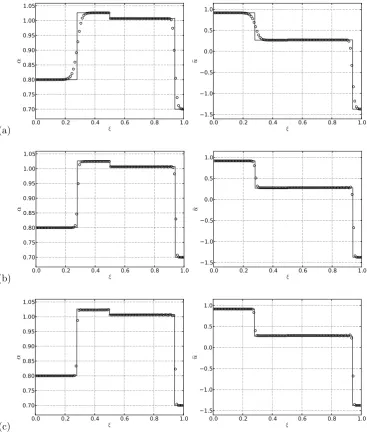
to inflate it. The emptying due to gravity generates a supercritical flow in the upstream portion of the vessel, while downstream boundary conditions impose subcritical flow. Connection of both conditions is achieved via an elastic jump. The problem was solved using a second order ADER scheme with a CFL numberCF L= 0.9 for both formulations, the conservative and the non-conservative ones. Figure 2.3 shows discrepancies between numerical solutions during the transient phase, deriving from observations made in section 2.3.3. The same discrepancies are found when the stationary solution is reached (figure 2.4).

0.0 0.2 0.4 0.6 0.8 1.0

ξ

0.0 0.5 1.0 1.5 2.0

α

Time = 1.6 s C

NC

0.0 0.2 0.4 0.6 0.8 1.0

ξ

−4 −2 0 2 4

u

[

m/s

] CNC

Figure 2.3: Giraffe jugular vein collapse test. Solution at output time t = 1.6s, during the transient phase. C: conservative formulation; NC: non-conservative formulation.

0.0 0.2 0.4 0.6 0.8 1.0

ξ

0.0 0.5 1.0 1.5 2.0

α

Time = 40.0 s C

NC

0.0 0.2 0.4 0.6 0.8 1.0

ξ

−4 −2 0 2 4

u

[

m/s

] CNC

Figure 2.4: Giraffe jugular vein collapse test. Solution at output timet= 40.0s, corresponding to the steady solution. C: conservative formulation; NC: non-conservative formulation.

In the next section we analyse a further aspect of the mathematical model which may have profound consequences in the design of a robust and accurate numerical scheme for solving system (2.1), namely the source term.

2.4

Source term stiffness

If we consider source terms, such as gravitational forces and dissipation due to viscous forces, system (2.1) can be rewritten as

(34)

where Qis given in (2.18) and the flux vectorF(Q) is (2.19). The source term is given by

S(Q) =

0

Ag−Ru

. (2.35)

The functionR is obtained from an assumed velocity profile; here we adopt the one proposed in [132]

R= 8πνA

1 2

ref

A12

, (2.36)

whereν is the kinematic viscosity andAref is a reference cross-sectional area. IfAref =Aone

recovers the friction term for tubes which when collapsing maintain a circular shape. When setting Aref =A0, R represents the friction term for a tube that assumes an elliptical shape

during collapse (as for highly compliant vessels, such as veins).

In this section we concentrate our attention on the study of the stiffness of the source term. A source term can be considered stiff if

∆t maxi{|βi|}>1, i= 1, . . . , N, (2.37)

whereβiis thei-th eigenvalue of the Jacobian of (2.35),∂S_∂(_QQ), andNis the number of unknowns

of the system.

Assuming a CFL-number CF L = 1 we can express relation (2.37) in terms of ratios be-tween the eigenvalues of the dissipative/productive process and the characteristic speeds for the advective process, namely

∆xmaxi{|βi|} maxi{|λi|}

>1. (2.38)

See [64]. Replacing (2.36) in source term (2.35) gives

S(Q) =

"

0

gq1−8πνA

1 2

0

u

A12

#

. (2.39)

Its Jacobian is

∂S(Q)

∂Q =

"

0 0

g+ 12πνA

1 2

0

u

A32

−8πνA

1 2

0 1

A32

#

. (2.40)

The eigenvalues of (2.40) are

β1= 0, β2=−8πνA

1 2

0 1

A32

=−8πν 1

α12A. (2.41)

We carry out an approximate analysis of the order of magnitude of ratio (2.38) for physiological values of the parameters involved withA:O(10−4_÷₁₀−7_),_u_:_O₍₁₀0_),_c_:_O₍₁₀0_),_ν _:_O₍₁₀−6_).

We obtain

∆x

8πν 1

α12A

u+c ≈∆x

O(101)O(10−6)

α12O(10−4_÷₁₀−7₎

O(100₎

≈O(10−1÷102)∆x

α12

.

(2.42)

The resulting ratio corresponds to a source term that may become stiff. The parameter αin (2.42) makes it evident that the collapse of a vessel may easily lead to an increase of (2.42) by one order of magnitude.

(35)

2.5

Concluding remarks

We have described a one-dimensional mathematical model for blood flow in large to medium-sized arteries and veins. Assuming constant material properties we have studied two possible formulations of the equations, a conservative and a non-conservative one. Then we have solved exactly the Riemann problem for both formulations and have assessed their suitability for various scenarios. We have in addition discussed the source terms present in both formulations and their potential stiffness, with the associated numerical complications.

(36)

(37)

Chapter 3

Numerical methods

There is an extensive literature on the numerical solution of one-dimensional blood flow models. All kinds of numerical methodologies were used to solve the underlying mathematical model: the finite-difference Lax-Wendroff scheme [41, 103]; the discontinuous Galerkin scheme [143, 2]; finite element schemes [164, 72] and finite volume schemes [58]. These references repre-sent some examples, but the available literature is extremely vast. In this chapter we describe the development of two high-order finite volume-type numerical schemes for one-dimensional blood