An edge texture features based methodology for bulk paddy variety recognition

An edge texture features based methodology for bulk paddy

variety recognition

Basavaraj S. Anami

_{, N. M. Naveen}

_{, N. G. Hanamaratti}

(1. Department of Computer Science and Engineering, K L E Institute of Technology, Hubli, 580030, India;

2. Department of Information Science and Engineering, K L E Institute of Technology, Hubli, 580030, India;

3. Department of Genetics and Plant Breeding, University of Agricultural Sciences, Dharwar, 580002, India)

Abstract: The paper presents a method for recognition of paddy varieties from their bulk grain sample edge images based on Haralick texture features extracted from grey level co-occurrence matrices. The edge images were obtained using Canny and maximum gradient edge detection methods. The average paddy variety recognition performances of the two categories of edge images were evaluated and compared. A feature set of thirteen texture features was considered and the feature set was reduced based on contribution of each feature to the paddy variety recognition accuracy. The average paddy variety recognition accuracy of 87.80% was obtained for the reduced eight texture features extracted from maximum gradient edge images. The work is useful in developing a machine vision system for agriculture produce market and developing multimedia applications in agriculture sciences.

Keywords: paddy, canny, sobel, texture features, feature extraction, ANN, pattern recognition

Citation: Anami, Basavaraj S., N. M. Naveen, and N. G. Hanamaratti. 2016. An edge texture features based methodology for bulk paddy variety recognition. Agric Eng Int: CIGR Journal, 18(1):399-410.

1 Introduction

India is an agriculture based country which decides

its economy. Agriculture sector contributes around 26%

of the gross domestic product (GDP). Paddy, jowar,

wheat, sugarcane, maize are few major crops in different

parts of India. Paddy is one of the most important

universal cereal grain crops and it is grown in all the

continents except Antarctica. India is the second largest

producer of wheat and paddy. India and China are

competing to establish the world record on rice yields.

Its cultivation is of immense importance to food security

of Asia, where more than 90% of the global rice is

produced and consumed.

Human beings recognize the paddy varieties during

quality evaluation and cultivation. The grain quality,

yield, resistance to pests and diseases, tolerance to

Received date: 2015- 09-06 Accepted date: 2015-11-04

*Corresponding author: N. M. Naveen, Asst. Professor, Department of ISE, K L E Institute of Technology, Hubli – 580030. E-mail: [email protected].

environmental stresses, farm input requirement, the

production of rice, rice flakes and puffed rice and pricing,

all these depend upon the variety. At present paddy grain

handling operation is carried out manually (also referred to

as visual inspection) by the trained personnel and is

considered as time consuming and moreover subjective.

These shortcomings of manual approach demand for the

development of a machine vision system to automatically

carry out recognition of paddy variety. This automation

would benefit the potential farmers in getting their right

price and right variety for cultivation. In order to know

the state-of-the-art in automation of such activities in the

field of agriculture, we have carried out a survey and the

gist of papers given under is divided into two broad

categories, one paddy related and the other allied.

Mousavi et al. (2014) presented an algorithm to

classify five different varieties of rice from unshelled

singleton kernel using the color and texture features. The

method used a feed-forward neural network classifier for

recognition of rice varieties and obtained 96.67% accuracy.

algorithm for classification of bulk paddy, brown and

white variety using 36 color features in RGB, HSI and

HSV color spaces. The algorithm adopted back

propagation neural network for classification and obtained

a mean classification accuracy of 96.66% with 13 color

features. Pazoki et al. (2014) proposed a methodology

for the classification of five paddy grain varieties using 24

color features, 11 morphological features and four shape

features. The features extracted from color images of

singleton grains of paddy gave classification accuracies of

99.46% and 99.73% for multi-layer perceptron (MLP) and

neuro-fuzzy classifiers respectively. Archana et al. (2014)

proposed an algorithm to classify four paddy varieties from

shape and texture features using artificial neural network.

The algorithm gave accuracies of 82.61%, 88.00%, and

87.27% for texture, shape and texture and shape features

respectively. The algorithm used singleton paddy grain

images. Mousavi et al. (2012) presented image processing

techniques to identify five different classes of unshelled

rice varieties using ensemble classifier. The forty-one

morphological features used to train ANN classifier gave

99.86% recognition accuracy. Pourreza et al. (2012)

applied machine vision techniques for the classification of

wheat varieties using one hundred and thirty one texture

features. The features included were GLCM (gray level

co-occurrence matrix), GLRM (gray level run-length

matrix), LBP (local binary patterns), LSP (local similarity

patterns) and LSN (local similarity numbers). The

deployed LDA (linear discriminate analysis) classifier gave

an average classification accuracy of 98.15%. The results

revealed that LSP, LSN and LBP features had significant

influence on classification accuracy. Guzman et al. (2008)

proposed a machine vision system based on neural

networks for automatic identification of five paddy

varieties of Philippines based on morphological features.

The method gave a classification accuracy of 70%.

Savakar (2010) illustrated an algorithm for

recognition and classification of similar looking grain

images using back propagation artificial neural network.

The method gave accuracy in the range 78%-84% for

individual color and texture features and in the range

85%-90% for combined color and texture features. Anami

et al. (2009) presented a methodology to identify the

different grain types from image samples of tray containing

multiple grains using color and textural features. A back

propagation neural network was used for identification of

bulk food grains using eighteen color and texture features.

Five different types of grains namely, alasandi, green gram,

metagi, red gram and wheat were tested and identification

accuracies observed in this work were 94% and 80% for

wheat and alasandi. Anami et al. (2005) developed a

Neural network approach for classification of single grain

kernels of different grains like wheat, maize, groundnut,

redgram, greengram and blackgram based on color, area

covered, height and width. The minimum and maximum

classification accuracies reported were 80% and 90%

respectively. Anami et al. (2009) presented different

methodologies devised for recognition and classification

of images of agricultural/horticultural produce based on

BPNN using color, texture and morphological features

with 87.5% accuracy. Huang et al. (2004) proposed an

identification method based on Bayes’ decision theory to

classify rice variety from individual grain samples using

color and shape features with 88.3% accuracy. Visen et

al. (2004) proposed combined color and texture features

based methodology to identify grain type from color

images of bulk grains using back propagation neural

network. A feature set consisting of 154 features was

reduced to 20. Classification accuracies of over 98% were

obtained for five grain types, namely barley, oats, rye,

wheat, and durum wheat for combined ten color features

and ten texture features, Paliwal et al. (2004) proposed a

robust algorithm for classifying images of bulk samples of

barley, wheat, oats, and rye using a four layer back

propagation neural network and obtained classification

accuracy of 99% using combined color and texture features.

Shearer and Holmes (1990) proposed a method for

identifying plants based on color texture characterization of

canopy sections. Color co-occurrence matrices were

saturation, and hue giving 11 texture features. The LDA

with 33 color texture features were used to identify plants.

Overall classification accuracy of 91% was obtained.

From the literature survey, it is observed that there is

some amount of research carried related to recognition and

classification of paddy grains and rice kernels. The

published work has mainly focused on classification of

paddy grains in singleton and non-touching grains. The

number of varieties is small. The morphological, color,

texture and shape features are employed in the works.

The size of the feature set adopted is large and amounts to

increased computational overhead during classification of

bulk paddy grains. Further, limited work is noticed on

variety identification from bulk samples of paddy grains.

This is the motivation for the present work, with an aim to

devise a smaller feature set, based on edge texture features

for variety recognition from bulk paddy grain sample

images.

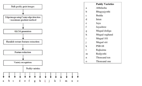
2 Proposed methods

The proposed method consists of four stages, namely,

image acquisition, edge detection, feature extraction,

feature selection and paddy variety recognition as shown

in Figure 1. The bulk sample edge images of fifteen

paddy grain varieties and Haralick texture features are

considered. A multilayer feed-forward artificial neural

network is used as recognizer of paddy varieties.

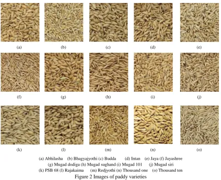
2.1 Image acquisition

In consultation with the University of Agricultural

Sciences (UAS), Dharwad, Karnataka State, India, fifteen

certified and popular paddy varieties are selected as grain

samples in the work. The paddy varieties are obtained

from Agricultural Research Station, Mugad, Dharwad.

These varieties are grown in different parts of Karnataka,

India. The varieties considered in the work include

Abhilasha, Bhagyajyothi, Budda, Intan, Jaya, Jayashree,

Mugad dodiga, Mugad sughand, Mugad 101, Mugad siri,

PSB 68, Rajkaima, Redjyothi, Thousand one and

Thousand ten. The images of paddy varieties are shown

in Figure 2.

Paddy Varieties

a Abhilasha b Bhagyajyothi

c Budda

d Intan

e Jaya

f Jayashree g Mugad dodiga h Mugad sughand i Mugad 101 j Mugad siri k PSB 68 l Rajkaima m Redjyothi n Thousand ten o Thousand one

A total 3000 images, considering 200 images from

each type of 15 paddy varieties are acquired under

standard lighting conditions using color camera PENTAX

MX-1, USA, having resolution of 14 mega pixels. In

order to provide a stable support and easy vertical

movement, the camera is mounted on a tripod stand as

shown in Figure 3. The images are taken keeping

approximately the object distance of 0.5 m. The acquired

images of size 1920 pixels  1080 pixels are resized to

400 pixels



computational overhead and storage requirements.

Figure 3 Image acquisition setup

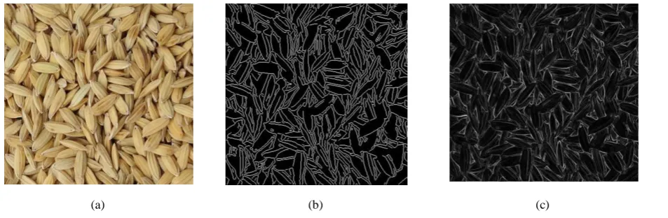
2.2 Edge detection

The edges in bulk sample ofpaddy grain images are

considered to be the most important image attributes that

exhibit different texture properties as shown in Figure 4

and provide valuable information for paddy variety

identification. This is the reason for adopting texture

analysis of edge images for paddy variety identification

from their bulk samples. Two standard edge detection

methods namely, Canny and maximum gradient method

are used to obtain edge images from RGB bulk paddy

grain image samples. The Canny edge detection method

basically finds edges where the grayscale intensity of the

image changes the most as shown in Figure 4b. These

areas are found by determining gradients of the image.

The maximum gradient method determines gradients at

each pixel in the image by applying Sobel operator and

returns edges at those points where the gradient of the

image is the maximum. The maximum gradient edge

(a) (b) (c) (d) (e)

(f) (g) (h) (i) (j)

(k) (l) (m) (n) (o)

(a) Abhilasha (b) Bhagyajyothi (c) Budda (d) Intan (e) Jaya (f) Jayashree (g) Mugad dodiga (h) Mugad sughand (i) Mugad 101 (j) Mugad siri (k) PSB 68 (l) Rajakaima (m) Redjyothi (n) Thousand one (o) Thousand ten

image is shown in Figure 4c. It is clear from Figure 4b

and Figure 4c that the maximum gradient edge detection

method is able to detect more edges than the Canny edge

detection method.

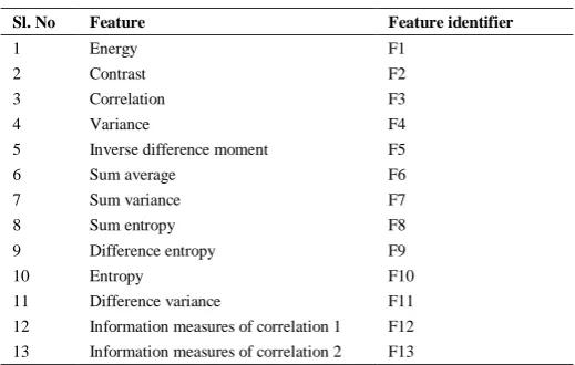
2.3 Feature extraction

From the edge images obtained using Canny and

maximum gradient edge detection methods, thirteen

Haralick texture features are extracted using gray level

co-occurrence matrix method (GLCM) and the texture

features are listed in Table 1. The GLCM Pφ, d (i, j)

represents a matrix of relative frequencies describing how

frequency pair of gray levels (i, j) appear in the window

separated by a given distance d = (dx, dy) at an angle ‘φ’.

Gray level co-occurrence matrices (GLCMs) method

counts how often pairs of gray level of pixels separated by

certain distance and oriented in a certain direction, while

scanning the image from left-to-right and top-to-bottom.

In the present work, a distance of 1 (d=1) when ‘φ’ is 0° or 90° and √2 (d= √2) when ‘φ’ is 45° or 135° has been

considered. The procedure of computing the

co-occurrence matrix is given in the Algorithm 1.

Algorithm 1: Computation of co-occurrence matrix

Pφ, d (i, j) from the image P (i, j)

Input: Color (RGB) image.

Output: Co-occurrence matrix Pφ, d(i, j) for d=1 in the

direction ‘φ’.

Start

Step 1: Convert input color image to gray level image

P (i, j)

Step 2: Assign Pφ, d (i, j) =0 for all i, j Є [0, L], where

‘L’ is the maximum gray level

Step 3: For all pixels (i1, j1) in the image, determine

(i2, j2), which is at distance ‘d’ in direction ‘φ’ of (00, 450,

900, and 1350) and compute P(i, j) | p (i1, j1), p (i2, j2)| =

Pφ, d |p (i1, j1), p (i2, j2)| + 1

Step 4: Compute Pφ, d = (p0, d + p45, d + p90, d + p135,

d)

Stop.

In order to define Haralick features, GLCM is

normalized as given in the Equation (1).

( ) ( )

∑ ∑ ( ) (1)

Where,

Px (i) = ∑ - ( ) (2)

Py (j) = ∑ ( )

-

(3)

Where, Px (i) and Py (i) are marginal probability

matrices, P(i, j) is the image attribute matrix, p(i, j, 1, 0)

represents the intensity co-occurrence matrix, Ng is total

number of intensity levels.

The Haralick features are defined as follows.

The angular moment (F1) or energy measures image

uniformity.

∑ ∑ [〖 ( )]〗

( )

(a) (b) (c)

(a) Original RGB image (b) Canny edge image (c) Maximum gradient edge image

Contrast (F2) measures intensity or gray level

variations between the pixel and its neighborhood.

∑ ∑ ( ) (5)

Where,

k=0, 1, 2……., 2 (Ng - 1)

Correlation (F3) measures intensity linear

dependence of gray level values to its neighborhood. Here,

μxandμyare the means and σx and σy are the standard

deviations of Pxand Pyrespectively.

(∑ ∑ ( )

) (6)

The sum of squares (F4) is defined by

∑ ∑ ( ) ( ) (7)

Where, is the mean gray level of the image.

Inverse difference moment (F5) is generally called

homogeneity that measures local homogeneity of the

image.

∑

∑

( )

( )

The sum average feature (F6) is defined by

∑ ( )

( )

(9)

The sum variance feature (F7) is defined by

∑ ( )( ) ( ) (10)

The sum and difference entropies (F8 and F9) are defined

by

∑ ( ) ( ) ( ) (11)

∑ ( )

( ) (12)

The entropy feature (F10) measures randomness of

intensity in the image defined by

∑ ∑ ( ) ( ) (13)

The difference variance (F11) is defined by

(14)

The information measures of correlation (F12 and F13) are

defined by

( ) ( ( )) (15)

[ ( )_{] (16)}

Where,

∑ ( ) ( ) (17)

∑ ∑ ( ) [ ( ) ( )] (18)

∑ ∑ ( ) ( ) [ ( ) ( )] (19)

The procedure used in obtaining the texture features

based on co-occurrence matrix is given in the Algorithm 2

and the Equations (4) to (16) are being used in the

algorithm to extract Haralick texture features. The features

are listed in Table 1.

Algorithm 2: GLCM texture feature extraction

Input: Color (RGB) image.

Output: Texture features.

Description: Pφ, d (i, j) means GLCM matrices in the

direction φ = 00, 450,900, and 1350 and ‘d’ is the distance.

Start

Step 1: Compute the co-occurrence matrix which is

independent of direction using

Algorithm 1

Step 2: Calculate co-occurrence texture features using

Equations (4) through (16)

Stop.

Table 1 Haralick texture features

Sl. No Feature Feature identifier

1 Energy F1

2 Contrast F2

3 Correlation F3

4 Variance F4

5 Inverse difference moment F5

6 Sum average F6

7 Sum variance F7

8 Sum entropy F8

9 Difference entropy F9

10 Entropy F10

11 Difference variance F11

12 Information measures of correlation 1 F12

13 Information measures of correlation 2 F13

2.3.1 Canny edge texture features extraction

Thirteen Haralick texture features are extracted from

the Canny edge images of all the fifteen paddy varieties

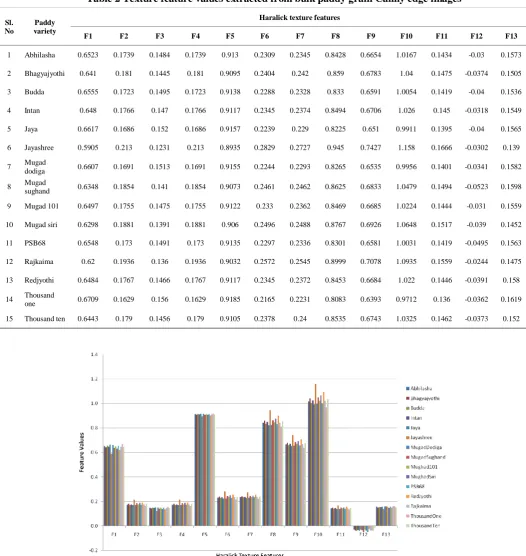
and the feature values are given in Table 2. The

graphical representation of the texture feature values with

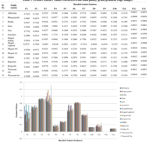
2.3.2 Gradient edge texture features extraction

Thirteen Haralick texture features are extracted from

the gradient edge images of all the fifteen paddy varieties

and the feature values are given in Table 3. The

graphical representation of the texture feature values with

respect to different paddy varieties are shown in Figure 6.

Table 2 Texture feature values extracted from bulk paddy grain Canny edge images

Sl. No

Paddy variety

Haralick texture features

F1 F2 F3 F4 F5 F6 F7 F8 F9 F10 F11 F12 F13

1 Abhilasha 0.6523 0.1739 0.1484 0.1739 0.913 0.2309 0.2345 0.8428 0.6654 1.0167 0.1434 -0.03 0.1573

2 Bhagyajyothi 0.641 0.181 0.1445 0.181 0.9095 0.2404 0.242 0.859 0.6783 1.04 0.1475 -0.0374 0.1505

3 Budda 0.6555 0.1723 0.1495 0.1723 0.9138 0.2288 0.2328 0.833 0.6591 1.0054 0.1419 -0.04 0.1536

4 Intan 0.648 0.1766 0.147 0.1766 0.9117 0.2345 0.2374 0.8494 0.6706 1.026 0.145 -0.0318 0.1549

5 Jaya 0.6617 0.1686 0.152 0.1686 0.9157 0.2239 0.229 0.8225 0.651 0.9911 0.1395 -0.04 0.1565

6 Jayashree 0.5905 0.213 0.1231 0.213 0.8935 0.2829 0.2727 0.945 0.7427 1.158 0.1666 -0.0302 0.139

7 Mugad

dodiga 0.6607 0.1691 0.1513 0.1691 0.9155 0.2244 0.2293 0.8265 0.6535 0.9956 0.1401 -0.0341 0.1582

8 Mugad

sughand 0.6348 0.1854 0.141 0.1854 0.9073 0.2461 0.2462 0.8625 0.6833 1.0479 0.1494 -0.0523 0.1598

9 Mugad 101 0.6497 0.1755 0.1475 0.1755 0.9122 0.233 0.2362 0.8469 0.6685 1.0224 0.1444 -0.031 0.1559

10 Mugad siri 0.6298 0.1881 0.1391 0.1881 0.906 0.2496 0.2488 0.8767 0.6926 1.0648 0.1517 -0.039 0.1452

11 PSB68 0.6548 0.173 0.1491 0.173 0.9135 0.2297 0.2336 0.8301 0.6581 1.0031 0.1419 -0.0495 0.1563

12 Rajkaima 0.62 0.1936 0.136 0.1936 0.9032 0.2572 0.2545 0.8999 0.7078 1.0935 0.1559 -0.0244 0.1475

13 Redjyothi 0.6484 0.1767 0.1466 0.1767 0.9117 0.2345 0.2372 0.8453 0.6684 1.022 0.1446 -0.0391 0.158

14 Thousand

one 0.6709 0.1629 0.156 0.1629 0.9185 0.2165 0.2231 0.8083 0.6393 0.9712 0.136 -0.0362 0.1619

15 Thousand ten 0.6443 0.179 0.1456 0.179 0.9105 0.2378 0.24 0.8535 0.6743 1.0325 0.1462 -0.0373 0.152

2.4 Feature selection

In order to reduce the computational overhead, the

feature set is reduced. The useful features that contribute

to the recognition process are selected by testing each

individual texture feature for paddy variety recognition

and performance feature selection is carried out. The

procedure for selecting significant features is given in

Algorithm 3.

Algorithm 3: Recognition performance based texture

feature selection.

Input: Extracted texture features along with their

respective average recognition accuracies (PARA ).

Output: Reduced feature sets with selected features.

Start

Step 1: Find out minimum and maximum average

recognition accuracies in all the texture features.

X = MINIMUM(PARA) // Minimum average

recognition accuracy in all the texture features

Y = MAXIMUM(PARA) // Maximum average

recognition accuracy in all the texture features Table 3 Texture feature values extracted from bulk paddy grain gradient edge images

Sl. No

Paddy variety

Haralick texture features

F1 F2 F3 F4 F5 F6 F7 F8 F9 F10 F11 F12 F13

1 Abhilasha _{0.7252 0.7301} 0.9193 0.9399 0.1666 0.2818 0.5718 0.8045 0.4681 0.1248 0.1516 -0.0011 0.0873

2 Bhagyajyothi _{0.4681 0.6674} 0.9112 0.9977 0.1550 0.2981 0.5955 0.8079 0.4756 0.1260 0.1761 -0.0009 0.0830

3 Budda _{0.5017 0.7162} 0.9424 0.8701 0.1733 0.2617 0.7242 0.8305 0.4566 0.1268 0.1385 -0.0011 0.0869

4 Intan _{0.5994 0.6984} 0.9206 1.0994 0.1417 0.2645 0.7659 0.8343 0.4905 0.1303 0.1940 -0.0011 0.0861

5 Jaya _{0.7742 0.6924} 0.9277 0.8460 0.1948 0.2974 0.5688 0.7967 0.4513 0.1219 0.1416 -0.0011 0.0869

6 Jayashree _{0.2884 0.6215} 0.8912 1.1774 0.1328 0.2963 0.6100 0.8182 0.5003 0.1297 0.2111 -0.0007 0.0789

7 Mugad

dodiga 0.5816 0.7149 0.9397 0.9040 0.1696 0.2609 0.7398 0.8332 0.4618 0.1275 0.1475

-0.0011 0.0872

8 Mugad

sughand 0.5572 0.7548 0.9497 0.8149 0.1853 0.2637 0.7314 0.8295 0.4476 0.1257 0.1214

-0.0013 0.0908

9 Mugad 101 _{0.5394 0.6772} 0.9231 0.9552 0.1616 0.2745 0.6194 0.8139 0.4702 0.1262 0.1551 -0.0010 0.0841

10 Mugad siri _{0.3699 0.6849} 0.9274 1.0307 0.1513 0.2685 0.7507 0.8307 0.4812 0.1291 0.1759 -0.0010 0.0855

11 PSB68 _{0.7551 0.7387} 0.9421 0.7666 0.2086 0.2876 0.5951 0.8013 0.4381 0.1211 0.1186 -0.0012 0.0892

12 Rajkaima _{0.3812 0.7022} 0.9195 0.9758 0.1658 0.2849 0.6396 0.8160 0.4711 0.1263 0.1668 -0.0009 0.0840

13 Redjyothi _{0.5461 0.6897} 0.8778 1.3231 0.1101 0.2874 0.6615 0.8223 0.5173 0.1320 0.2545 -0.0011 0.0863

14 Thousand

one 0.5567 0.6932 0.9180 0.9342 0.1777 0.3001 0.5842 0.7995 0.4657 0.1236 0.1618

-0.0011 0.0857

15 Thousand ten _{0.5200 0.6920} 0.9271 0.9356 0.1706 0.2796 0.6625 0.8194 0.4653 0.1262 0.1554 -0.0010 0.0855

Step 2: Compute recognition accuracy threshold

(RAT) value.

RAT = (X + Y)/2

Step 3: Compare the average recognition accuracies

of all the features with RAT.

Construct reduced feature set by selecting the texture

features whose average recognition accuracies are equal to

or greater than the RAT value.

Step 4: Compare, if RAT <= Y, then X = RAT and go

to Step 2 else return the reduced feature sets.

End

2.5 Recognition of paddy varieties

A multilayer feed-forward neural network is

considered for paddy variety recognition. The number of

neurons in the input layer is set to the number of

appropriate texture features selected as input and the

output layer is set to 15. Levenberg-Marquardt (LM)

back propagation algorithm is used for the training. The

termination error (TE) is set to 0.01, learning rate (η) is set

to 0.05 and momentum coefficient (µ) is set to 0.6. The

sigmoid activation functions are used in the hidden layers.

The network is trained and tested for 1000 epochs. With

these parameters, the network is trained. Once the

training is complete, the test data for each of the paddy

variety is tested. The overall recognition process is given

in Algorithm 4.

Algorithm 4: Overall recognition of paddy varieties

from bulk grain sample images using color texture

features.

Input: Bulk paddy sample images of different

varieties.

Output: Recognized paddy variety

Start

Step 1: Convert color (RGB) input images into

(Canny/Gradient) edge images.

Step 2: Compute co-occurrence matrix (GLCM) for

the edge images using Algorithm 1.

Step 3: Extract texture features of the edge images

using Algorithm 2.

Step 4: Perform feature selection using Algorithm 3

Step 5: Train artificial neural network (ANN) with

the selected texture feature set obtained in Step 4.

Step 6: Accept test image and extract the selected

texture features using Algorithm 3.

Step 7: Recognize the image containing bulk paddy

sample using ANN classifier. Repeat the steps 6 and 7 for

all the test images.

End

3 Results and discussion

The software tool MATLAB 7.11.0 is used to

implement the devised algorithms. A total of 3000 image

samples, 200 images of each varietal type are considered.

Out of these image samples 1500 images (100 images of

each paddy variety) are used for training and 1500 images

(100 images of each paddy variety) are used for testing.

The percentage of recognition accuracy as the ratio of total

number of correctly recognized test image samples to the

total number of test image samples is given by the

Equation (20). The average recognition accuracy (PARA)

is calculated as the ratio of sum of recognition accuracies

of all the paddy varieties to the total number of paddy

varieties considered and is given by the Equation (21).

(20)

Where, PA is the percentage of recognition accuracy (%);

TC is the total number of correctly recognized images; and

TT is the total number of test images.

∑

(21)

Where, PARA is Average recognition accuracy (%);i is the

variety order number; percentage of recognition

accuracy of ith variety; and TN is the total number of the

paddy varieties.

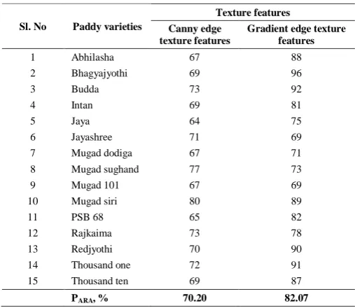
3.1 Variety recognition using canny edge texture

features

The training and testing processes are carried out

using texture features extracted from the Canny edge

texture features are considered for the paddy recognition

process and obtained average variety recognition accuracy

of 70.20% across 15 paddy varieties as given in Table 4.

Table 4 Paddy variety recognition using edge texture features

Sl. No Paddy varieties

Texture features

Canny edge texture features

Gradient edge texture features

1 Abhilasha 67 88

2 Bhagyajyothi 69 96

3 Budda 73 92

4 Intan 69 81

5 Jaya 64 75

6 Jayashree 71 69

7 Mugad dodiga 67 71

8 Mugad sughand 77 73

9 Mugad 101 67 69

10 Mugad siri 80 89

11 PSB 68 65 82

12 Rajkaima 73 78

13 Redjyothi 70 90

14 Thousand one 72 91

15 Thousand ten 69 87

PARA, % 70.20 82.07

3.2 Variety recognition using gradient edge texture

features

The training and testing processes are carried out

using texture features extracted from the gradient edge

images of bulk sample of 15 paddy varieties. Initially, 13

texture features are considered for the paddy recognition

process and obtained average variety recognition accuracy

of 82.07% across 15 paddy varieties as given in Table 4.

It is observed from the Table 4 that the gradient edge

texture features give better average recognition accuracy

over canny edge texture features. So we have adopted

gradient edge texture features for paddy variety

identification.

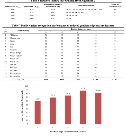
In order to improve the recognition accuracy of

gradient edge texture features, the performance based

feature selection operation is carried out using Algorithm

3. The recognition accuracies of all the individual

gradient edge texture features are evaluated as input to the

algorithm and the recognition accuracies are given in

Table 5. The reduce feature sets and their sizes obtained

using the algorithm are given in Table 6. The reduced

feature sets are trained and tested using ANN and the

obtained results are given in Table 7. From Table 7, the

highest average recognition accuracy of 87.80% is

obtained for the reduced feature set with size 11 and the

paddy variety Abhilasha gives the highest recognition

accuracy of 96% and lowest is obtained for the paddy

variety PSB 68. The recognition performances of all the

reduced gradient edge texture feature sets are graphically

shown in Figure 7.

Table 5 Paddy variety recognition performance of individual gradient edge texture feature

Sl. No

Paddy varieties

Gradient edge texture features

F1 F2 F3 F4 F5 F6 F7 F8 F9 F10 F11 F12 F13

1 Abhilasha 53 26 31 45 41 33 42 49 45 66 46 1 16

2 Bhagyajyothi 57 30 33 49 45 37 43 57 51 55 37 6 12

3 Budda 50 23 29 55 41 41 36 48 58 49 33 7 21

4 Intan 48 36 32 52 47 28 47 50 51 67 36 3 28

5 Jaya 47 41 36 53 51 31 42 54 67 77 42 11 23

6 Jayashree 45 24 24 51 43 33 37 58 62 47 36 3 19

7

Mugad

dodiga 47 28 20 51 46 36 33 56 63 56 33 21 22

8

Mugad

sughand 46 31 38 49 44 44 38 52 55 55 31 1 26

9 Mugad 101 51 33 41 38 46 35 31 57 49 49 26 5 24

10 Mugad siri 49 37 22 43 51 40 45 54 52 53 29 10 29

11 PSB 68 52 40 37 40 49 31 42 49 40 47 36 6 16

12 Rajkaima 49 28 37 47 46 30 38 54 44 45 41 2 19

13 Redjyothi 52 38 32 39 49 27 32 50 62 58 25 16 31

14 Thousand ten 51 29 35 47 47 37 35 55 39 65 35 2 26

15

Thousand

one 55 30 33 29 50 29 41 44 54 50 30 9 30

The proposed method has considered fifteen paddy

varieties, which is three times more than the reported work

and the number of features considered is less than the

features used in the reported work as depicted in Table 8. Table 6 Reduced feature sets obtained from Algorithm 3

Y

(Maximum PARA)

X

(Minimum PARA)

Recognition accuracy

threshold (RAT) Reduced feature sets

Reduced feature set size

55.93 6.87 31.40 F1, F2, F3, F4, F5, F6, F7, F8, F9, F10, F11 11

55.93 31.40 43.67 F1, F4, F5, F8, F9, F10 6

55.93 43.67 49.80 F1, F8, F9, F10 4

55.93 49.80 52.87 F9, F10 2

Table 7 Paddy variety recognition performance of reduced gradient edge texture features

Sl.

No Paddy variety

Reduce feature set sizes

2 4 6 11 13

1 Abhilasha 54 65 68 96 88

2 Bhagyajyothi 59 72 84 94 96

3 Budda 60 69 82 92 92

4 Intan 51 66 77 90 81

5 Jaya 66 77 75 89 75

6 Jayashree 59 73 69 85 69

7 Mugad dodiga 62 71 72 80 71

8 Mugad sughand 58 74 69 84 73

9 Mugad 101 63 68 72 83 69

10 Mugad siri 60 77 79 87 89

11 PSB 68 56 66 72 79 82

12 Rajkaima 61 71 68 90 78

13 Redjyothi 68 69 76 87 90

14 Thousand one 73 72 79 91 91

15 Thousand ten 62 57 77 90 87

PARA , % 60.80 69.80 74.60 87.80 82.07

Figure 7 Graphical representation of gradient edge texture features performance in paddy variety recognition

Table 8 Comparison of proposed method with the literature

Literature Number of paddy varieties Sample type Features Accuracy (%)

(Guzman et al., 2008) 5 Singleton grain 13 morphological features 70.00

(Pazoki et al., 2014) 5 Singleton grain 24 color, 11 morphological, 4 shape features 99.73

(Golpur et al., 2014) 5 Bulk grains 13 color features 96.66

4 Conclusions

The Haralick texture features are used for the

recognition of 15 paddy varieties from their bulk sample

edge images. The Canny and maximum gradient edge

detection methods are applied to obtain the edge images.

The average recognition accuracy of 87.80% is obtained

for reduced 11 texture features extracted from maximum

gradient edge images which is better than the recognition

result obtained using the texture features extracted from

Canny edge images. The proposed method has

considered number of varieties three times more and

number of features used is nearly half than the reported

work. The results are encouraging. The work finds

application in developing a machine vision system for

agriculture produce market and developing multimedia

applications in agriculture sciences.

References

Anami, B. S., and D. G. Savakar. 2009. Recognition and Classification of Food Grains, Fruits and Flowers Using Machine Vision. International Journal of Food Engineering, 5(4): 1-25. Issue 4, Article 14.

Anami, B. S., D. G. Savakar, and S. B. Vijay. 2009. Identification of multiple grain image samples from tray. International journal of food science & technology, 44(12): 2452-2458.

Chaugule, A., and S. N. Mali. 2014. Evaluation of texture and shape features for classification of four paddy varieties. Journal of Engineering, Article ID 617263.

Anami, B. S., D. G. Savakar, A. Makandar, and P. H. Unki. 2005. A neural network model for classification of bulk grain samples based on color and texture. In Proceedings of International Conference on Cognition and Recognition. Mandya, India.

Canny, J. F. 1986. A computational approach to edge detection. IEEE Trans Pattern Analysis and Machine Intelligence, 8(6): 679-698.

Guzman, J. D., and E. K. Peralta. 2008. Classification of Philippine rice grains using machine vision and artificial

neural networks. In Iaald Afita WCCA World Conference on Agricultural Information and IT, 24-27. Tokyo, Japan. Golpour, I., Parian, J.A. and Chayjan, R. A. 2014. Identification and

classification of bulk paddy,brown and white rice cultivars with colour features extraction using image analysis and neuralnetwork, Czech Journal Food Science, 32(3): 280–287. Haralick, R.M., K. Shanmugam, and I.H. Dinstein. 1973. Textural features for image classification. Systems, Man and Cybernetics, IEEE Transactions on Vol. SMC-3(6): 610-621. Huang, X. Y., J. Li, and S. Jiang. 2004. Study on identification of rice varieties using computer vision. Journal of Jiangsu University (National Science Edition), 25(2): 102–104. Mousavi Rad, S. J., Tab, F. A., & Mollazade, K. 2014. Classification

of rice varieties using optimal color and texture features and BP neural networks. In Machine Vision and Image Processing (MVIP), 7th Iranian (pp. 1-5). IEEE.

Paliwal, J., M. S. Borhan, and D. S. Jayas. 2004. Classification of cereal grains using a flatbed scanner. Canadian Biosystems Engineering, 46: 1-3.

Pazoki, A. R., F. Farokhi, and Z. Pazoki. 2014. Classification of Rice Grain Varieties using Two Artificial Neural Networks (MLP and Neuro-Fuzzy). The Journal of Animal & Plant Sciences, 24: 336-343.

Pourreza, A., Pourreza, H., Abbaspour-Fard, M.H. and Sadrnia, H., 2012. Identification of nine Iranian wheat seed varieties by textural analysis with image processing. Computers and electronics in agriculture, 83:102-108.

Savakar, D. G. 2012. Recognition and Classification Of Similar Looking Grain Images Using Artificial Neural Networks. Journal of Applied Computer Science and Mathematics, 13. Shearer, S. A., and R. G. Holmes. 1990. Plant identification using

color co-occurrence matrices. Transactions of the ASAE, 33(6): 2037-2044.

Silva, C. S., and U. Sonnadara. 2013. Classification of Rice Grains Using Neural Networks. Proceedings of Technical Sessions, 29: 9-14.

Sobel, I., and G. Feldman. 1968. A 3x3 Isotropic Gradient Operator for Image Processing. Presented at the Stanford Artificial Intelligence Project (SAIL).