Parameter evaluation for soil erosion estimation on small watersheds using
SWAT model
Fiaz Hussain
1,2*,
Ghulam Nabi
3,
Ray-Shyan Wu
1,
Bashir Hussain
4,
Tanveer Abbas
3(1. Department of Civil Engineering, National Central University, Taiwan 32001, China; 2. PMAS-Arid Agriculture University Rawalpindi 46000, Pakistan;
3. Centre of Excellence in Water Resources Engineering, University of Engineering and Technology, Lahore 54890, Pakistan; 4. Soil and Water Conservation Research Institute (SAWCRI) Chakwal, Chakwal 48800, Pakistan)
Abstract: This research was undertaken for the evaluation of soil erosion using the semi-distributed basin scale SWAT model for four subcatchments of the Dhrabi River Catchment (DRC), which is located in the Pothwar Plateau region. Two subcatchments (catchment-25 and -31) are characterized by gullies while the other two (catchment-27 and -32) are managed with terraced landuse system. The performance of the model was satisfactory with coefficient of determination (R2) = 0.67 to 0.91 and Nash-Sutcliffe efficiency (ENS) = 0.54 to 0.85 for both surface runoff and sediment yield during the calibration (2009-
2010) and validation (2011) periods. The PUSLE factor was found to be the most sensitive parameter during model calibration.
It was observed that all of the rainfall- runoff events occurred during the monsoon season (June to September). The estimated annual sediment loss ranged from 2.6 t/hm2 to 31.1 t/hm2 over the duration of the simulation period for the non-terraced
catchments, in response to annual precipitation amounts that were between 194.8 mm to 579.3 mm. In contrast, the predicted annual sediment levels for the terraced catchments ranged from 0.52 t/hm2 to 10.10 t/hm2 due to similar precipitation amounts. The terraced catchments resulted in 4 to 5 times lower sediment yield as compared to non-terraced catchments. The results suggest that there is a huge potential for terraces to reduce soil erosion in the DRC specifically and Pothwar area generally, which have proven to be an efficient approach to establishing soil and water conservation structures in this region.
Keywords: SWAT modeling, sediment yield, Modified version of Universal Soil Loss Equation (MUSLE), calibration, validation, parameter evaluation, small watersheds
DOI: 10.25165/j.ijabe.20191201.3769
Citation: Hussain F, Nabi G, Wu R-S, Hussain B, Abbas T. Parameter evaluation for soil erosion estimation on small watersheds using SWAT model. Int J Agric & Biol Eng, 2019; 12(1): 96–108.
1 Introduction
Globally, problems related tosoil and water resources are a growing concern. It has been estimated that between 549-1094 million hm2 of land are affected by wind and water erosion, respectively[1,2]. The land degradation due to soil erosion is a severe problem which threaten the soil resources and agricultural productivity[3,4]. Borrelli et al.[5] predicted that the highest rates of soil erosion in Southeast Asia, Sub-Saharan Africa and South America occur in the least developed economies. According to Food and Agriculture Organization (FAO)[6], South Asia countries are losing at least 10 billion USD per year due to agricultural production losses occurring from land degradation. Annually, the global productivity loss ranges from 13 billion to 28 billion USD for dryland (rainfed cropland) production[7]. More than 10 billion
hm2 of land worldwide are experiencing severe soil degradation
Received date: 2017-08-29 Accepted date: 2019-01-13
Biographies: Ghulam Nabi, Assistant Professor, research interest: sediment
transport modeling, Email: [email protected]; Ray-Shyan Wu, Professor, research interest: water resources systems, Email: [email protected]; Bashir
Hussain, Assistant Agriculture Engineer, research interest: soil and water
conservation, Email: [email protected]; Tanveer Abbas, Master, research interest: hydrological modeling: Email: [email protected].
*Corresponding author: Fiaz Hussain, PhD candidate, research interest:
watershed hydrology and soil erosion modeling, Department of Civil Engineering, National Central University, Taiwan 32001. Tel: +886-905-787-554, Fax 886-3-425- 2960, Email: [email protected], [email protected].
due to water erosion, based on a global survey[8]. Current water erosion rates are accelerating at a second order of magnitude on arable land which creates a major imbalance between soil formation and soil loss by a factor 10-100[9,10]. The formation of new soil is a notoriously slow, gradual and continuous process as evidenced by the formation of one-inch of new topsoil, which requires 100-1000 years[11]. However, the rate varies widely, depending on climate, time, parent material, topography and living organisms. Globally, soil is being lost from land areas 10-40 times faster than the rate of renewal and annually about 10 million hm2 of cropland is lost due to soil erosion[12].
structures, increased the loss of fertile soil and vegetation, resulted in reservoir depletion, and surface and groundwater contamination.
Annual soil loss over different landuses in the Soan River catchment of the Pothwar region ranges from 18.70 t/hm2 to
63.5 t/hm2 using Morgan approach integrated with GIS and RS and it was estimated that the rate of soil erosion mainly depends on the nature of vegetation cover, overland flow and texture of the soil[16]. It was estimated that 75% area of the Dhrabi River Catchment (DRC) is impacted by soil erosion with mean rates of 82 t/hm2 using the Revised Universal Soil Loss Equation (RUSLE)[17] and Water Erosion Prediction Project (WEPP)[18,19] models[20]. This results in a high variability of soil fertility and productivity within the area, which diminishes the storage and filtering function of the soil[20]. Soil erosion is a three step process involving detachment, transportation and deposition which causes onsite as well as offsite problems. Onsite effects are the removal of organic matter and soil nutrients which reduce agriculture production. Offsite problems are often more severe include river silting, impaired water quality of reservoirs, reduced reservoir storage, and exacerbation of floods and landslides[21]. Due to these effects the soil and water resources are under threat and the productivity of land is decreasing which ultimately leads to a reduction in agricultural production. The accelerated soil erosion is a serious agro-environmental threat to food security and agriculture sustainability worldwide[3,22,23].
Topography, landuse/land cover (LULC), soil type, soil structure and climatic conditions are major related factors that influence soil erosion. Assessment of soil erosion at the catchment scale is a difficult task and is most realistically performed using available soil erosion modeling techniques including: (1) Universal Soil Loss Equation (USLE)[24], (2) physically-based models such as WEPP, (3) and a combination of empirical and physically based methods that are used in the Soil and Water Assessment Tool (SWAT)[25]. These tools can be very much helpful in implementing the planning and management of soil and water conservation projects.
SWAT exemplifies a compromise between empirical and physical algorithms; e.g., a modified version of USLE (MUSLE)[26]
that is used to simulate water erosion. Furthermore, it is considered a more suitable tool for agricultural management practices in watersheds, compared with other models[27]. It was developed in the early 1990s to assist water resource managers in assessing the impact of management and climate on water supplies and non-point source pollution in watersheds and large river basins[28], and can be used in small agricultural watersheds to
simulate water and soil loss[29-33]. SWAT is a watershed-scale ecohydrological model that has been tested for a wide variety of watershed scales and environmental conditions worldwide[34-39], and has been applied for an extensive range of climate change, landuse change, Best Management Practice (BMP) assessments and other scenario analyses. For example, Mosbahi et al.[40] used SWAT for soil erosion risk assessment to adopt the appropriate management intervention and recommended it for prioritization of vulnerable areas in semi-arid catchments. At present, roughly 3500 SWAT-related studies that were published between 1993 and 2018 have been identified in the literature [41].
Samad et al.[42] applied SWAT model for the assessment of sediment yield in Rawal Dam catchment of Pothwar region. The effectiveness of the model was evaluated with Nash and Sutcliffe coefficient (0.79). The hydrological modeling of Simly Dam watershed located in Soan River basin Pothwar region was studied
in 2015 using GIS and SWAT. The estimated water balance results revealed that the inflow was successfully reproduced with Coefficient of Determination (R2) of 0.75 and the author recommended that SWAT can be used efficiently in semi-arid regions to support water management policies[43]. To the best of our knowledge, the application of SWAT reported here is the first time that it has been applied for DRC subcatchments. Thus the specific objectives of this study were to: (1) test SWAT for four small subcatchments that are representative of typical DRC conditions, and (2) to evaluate soil erosion related parameters used in SWAT in the context of subcatchments that have been treated with terraces versus other subcatchments that do not have terraces.
2 Study area description
This study was conducted for four DRC subcatchments which are referred to as subcatchment-25, subcatchment-27, subcatchment-31 and subcatchment-32 (Figure 1). The DRC drains an area of 196 km² between latitudes 32°42ʹ36″N to 32°55ʹ48″N and longitudes 72°35ʹ24″E to 72°48ʹ36″E in District Chakwal, Pothwar, Pakistan. Precipitation is the main source of freshwater in the DRC. The undulating and uneven topography has deep to shallow gullies, large to small terraces and low to medium hills between elevations of 465-919 masl. The slope steepness varies from 2% in areas characterized by relatively flat plain conditions to >30% along the hillsides. The dominant soil type is a sandy loam that has low (<1%) organic matter. Generally, the climate is hot in the summer season and cold during the winter. The summer season extends from April to September, with the highest temperatures occurring during June and July (30°C-35°C). The winter season spans the months of October to March, with the coldest temperatures occurring in December and January (0°C-5°C). About 65%-70% of the annual precipitation occurs during the monsoon season (July to September) while the remaining 30%-35% of the annual precipitation occurs during the winter season (December to March). The average annual precipitation is about 630 mm[15]. The major landuse classifications of this area are: Agricultural Land (22%; 43 km2), Barren Land with Shrubs and Bushes (32%; 62 km2), Fallow/Range Land with Range Grasses (33%; 65 km2), Residential Areas (4%; 9 km2), Water Bodies (3%; 7.0 km2) and Forests (6%; 11 km2). The location of the DRC in Pakistan and the locations of the four DRC subcatchments are shown in Figure 1.
Figure 1 Location of study catchments within the Dhrabi River Catchment (DRC), and the location of the DRC within the Pothwar
In the Pothwar Plateau region, the agriculture fields are not flat and the crops are grown on terraces that consist of wide and deep gullies. The field terraces are situated at different elevation levels as shown in Appendix A (Figure A1). The terrace systems typically fail due to breaching of field embankments/bunds when intense precipitation events occur (Figure A2). Locally loose stone structures have thus been installed in clusters in the upper, middle, and lower parts of terraced catchments to help mitigate this problem (Figures A3-A5).
Subcatchments-25 and -31 are characterized by eroded gullies while terraces have been installed on subcatchments-27 and -32 (Figure 2). The gullies are visible with deep and wide beds while the terraces are installed in incised gullies with an average vertical interval of about 0.5 m. Subcatchments-25 and -27 are adjacent with each other having latitude 32.8948o to 32.8917o and longitude 72.70o to 72.71o. Subcatchments-31 and -32 are also adjacent with latitude 32.9188o to 32.9159o and longitude 72.7109o to
72.7100o. The soil type is sandy loam (67%-74% sand, 14%-22% silt and 10%-14% clay) in all four subcatchments and is calcareous in nature.
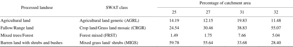
A physical topographical survey of the subcatchments was conducted using a Global Positioning System (GPS; eTrex Venture® HCx with accuracy <10 m, 95% typical). A DEM of each subcatchment was generated as a function of point source elevation data in GIS and the Inverse Distance Weighted (IDW) method[44,45] as shown in Figure 3. The IDW was used because it is popular deterministic method, and has been used at varying spatial and temporal scales because of simplicity. The landuse maps were generated using Google Earth[46] as shown in Figure 4. The landuse classifications of each subcatchment with the corresponding percentages of landuse area are given in Table 1.
a. Subcatchments-27 and -32 terraced landuse system
b. Subcatchment-25 and -31 gully landuse system
Figure 2 Subcatchments-27 and -32 terraced landuse system in incised permanent gullies and Subcatchments-25 and -31 gully
landuse system
Figure 4 Land use maps for the Dhrabi River catchment study subcatchments
Table 1 Landuse classification of the four subcatchments
Processed landuse SWAT class
Percentage of catchment area
25 27 31 32
Agricultural land Agricultural land generic (AGRL) 14.19 12.15 19.83 11.48
Fallow/Range land Crop land/Grass land mosaic (CRGR) 24.54 30.46 38.83 55.07
Mixed trees/Forest Forest mixed (FRST) 1.49 1.75 7.66 5.04
Barren land with shrubs and bushes Mixed grass land/ shrubs (MIGS) 59.78 55.64 33.68 28.40 The barren land with shrubs and bushes are used for grazing in
all four subcatchments, while the fallow/range land are converted and cultivated during the cropping season in catchment-27 and -32. The salient features of the study subcatchments are discussed below, which are fully representative of the DRC area and have well defined boundaries.
Subcatchment-25: The catchment contains a deep gully having a wide gully bed. The upslope portion of the gully has bushes, scrub trees and range grasses. The main crop grown during the winter season on the agricultural area is wheat. Subcatchment-25 has a total area of 2.0 hm2 with an average slope of 10.5% and elevation range of 527.1 m to 539.8 m.
Subcatchment-27: This subcatchment has an area of 3.0 hm2, with a total of 11 terraces that have been installed across a gully incision. The average vertical interval is about 0.5 m between the terraces. Arable crops such as winter wheat are grown on the terraces. The subcatchment elevation ranges between 528.3 m to 540 m with an average slope of 5.8%.
Subcatchment-31: The subcatchment is characterized by a gully incision with grass growing on the gully slopes. The area is 1.5 hm2 with an average slope of 10%. The elevation is between 509.15 m to 520.67 m.
Subatchment-32: This subcatchment has an area of 3.3 hm2 and 7.6% average slope. The incised gully bed has been modified with 13 terraces, with an average vertical interval of about 0.5 m
between the terraces, which are used for growing arable crops such as sorghum and millet mixed fodder and wheat during the winter season. The elevation ranges from 513.22 to 518.58 masl.
3 Materials and methods
3.1 Data required and collection
Three types of data were required for modeling sediment yield: (1) spatial/raster data including DEM, masked DEM, landuse, soil and slope data, and (2) daily meteorological data including precipitation, temperature (maximum and minimum) in a lookup table, and (3) observed runoff and sediment data.
yield measurement processes are given in Iqbal et al.[48]
Figure 5 Experimental setup for runoff and sediment yield
3.2 SWAT Model description
SWAT is a comprehensive, semi distributed, physically-based basin scale hydrological model used to predict the impact of landuse and agricultural management practices on water and sediment yield in large as well as small watersheds over long durations of time[25,49]. The ArcGIS SWAT (ArcSWAT)
interface[50,51] uses geographic information systems (GIS) spatial algorithms to spatially link multiple model input data, such as catchment topography (DEM), soil, land use, land management and climatic data. The delineation of a catchment into sub-catchments in ArcSWAT is performed on the basis of drainage area and topography. Typically, each sub-catchment is then further sub-divided into hydrological response units (HRUs) based on spatial uniformity in landuse, soil type and slope. The model computes surface runoff for each hydrologic response unit (HRU) by using the modified USDA-SCS curve number method[52] or Green and Ampt infiltration method[53]. Sediment yield from each HRU is estimated with the Modified Universal Soil Loss Equation (MUSLE)[26] as given in the following mass balance equation:
0.56
. 11.8( )
surf peak uru USLE USLE USLE
USLE
S Y Q q areah K C P
LS CFRG
(1)
where, S.Y = Sediment yield, t/hm2; Qsurf= Surface runoff, mm/hm2;
qpeak = Peak runoff rate, m3/s; areahru=Area of hydrological
response unit, hm2; KUSLE = USLE Soil erodibility factor; CUSLE =
USLE cover and management factor; PUSLE=USLE support
practice factor; LSUSLE = Slope length and slope steepness factor;
CFRG = Coarse fragment factor.
A detailed description of these and other components are available in the SWAT theoretical documentation[49].
3.3 SWAT Model setup and simulation
During the watershed delineation process in ArcSWAT, each of the four subcatchments was maintained as a single subbasin, because of the relatively small size of each subcatchment (from 1.5 hm2 to 3.3 hm2). Then, each of four subcatchments was discretized into HRUs, resulting in the following number of HRUs for subcatchments-25, -27, -31 and -32, respectively: 8, 12, 6 and 14. An appropriate database of subcatchment parameters and a comprehensive topographic report of the catchment are generated upon successful execution of the terrain processing module within the ArcSWAT interface. The respective look-up tables, land use and soil maps were supplied to the model for reclassification according to SWAT coding conventions. Further, the subcatchment was classified into different slope categories and HRUs with unique land cover, soil and slope classes by overlaying all three maps with the HRU threshold set at 0% to allow all of the original landuse, soil and slope data to be included in the creation of HRUs. This was necessary to prevent the loss of any of the
input data, which occurs when the HRU development thresholds are set at a non-zero percentage[54], and because SWAT pollution outputs are sensitive to the resolution of HRU and subcatchment delineations[34,54].
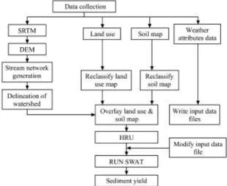
The weather station location table, and tables of daily precipitation and temperatures (maximum and minimum) data, were incorporated into the model setup and linked with the required input files. The surface runoff and sediment yield predicted by the un-calibrated model were initially compared versus different rainfall and sediment loss events on a daily basis using default parameter values. The general algorithm used for the sediment yield simulation for the four subcatchments is given in Figure 6. The initial un-calibrated simulation was saved as Sim1 which was further modified for model calibration.
3.4 SWAT calibration and validation
The determination of the most sensitive parameters for model calibration and validation was considered as the first step in this study[55]. The user determines which variables to adjust based on sensitivity analyses, literature data, local expertise and other relevant sources of information[56]. Sensitivity analysis is the rate of change in model output values with respect to changes in model input parameters. For determining the most sensitive parameter for model calibration the sensitivity analysis was performed in the ArcSWAT interface using five parameters for sediment yield[49]:
PUSLE, CUSLE, KUSLE, linear parameter for calculating the maximum
amount of sediment that can be re-entrained during channel sediment routing (SPCON), and the exponent parameter for calculating sediment re-entrained in channel sediment routing (SPEXP).
Figure 6 General algorithm used for sediment yield simulation for the four subcatchments
The final step is the model validation which was done by comparing the model results with observed data using climate data inputs for 2011. No additional parameter adjustments were performed during the validation period.
Figure 7 SWAT manual calibration flowchart used for surface runoff and sediment yield (from Engel et al.[57]; adapted from
Santhi et al.[58])
4 Model performance evaluation
Agreement between observed and simulated values is commonly assessed by using efficiency criteria such as the R2, Nash Sutcliffe Modeling Efficiency (ENS) and Index of Agreement
(d)[59]. The SWAT calibration and validation results were evaluated using the ENS and R2, which are the most widely used
statistical methods as previously reported by Gassman et al.[34,35]
and Bressiani et al.[39] The model performance was judged based on performance evaluation criteria (PEC) for catchment-scale models suggested by Moriasi et al.[60] their criteria state that satisfactory performance occurs on a daily, monthly and annual basis for a flow simulation if R2 >0.6 and ENS >0.5, and for a sediment prediction if R2 >0.45 and ENS >0.45.
4.1 Nash-Sutcliffe coefficient (ENS)
The ENS coefficient [59,61]
is a normalized statistic that indicates the efficiency of a model by relating the goodness-of-fit of the model’s predictions to the variance of the observed data. The ENS
provides a measure how well the simulated results match the observed data along a 1:1 line:
2 1 NS 2 0 1 ( ) E 1 ( ) n oi si i n oi i Q Q Q Q
(2)where, ENS is the Nash-Sutcliffe coefficient; Qoi is the observed
data; Qsi is the simulated data and Q0 is the average of observed data. The ENS ranges from –∞ to 1. ENS = 1 indicates a perfect
match between the simulated and observed data, ENS=0 indicates
that mean of the observed data is as accurate the simulated data, and ENS<0 occurs when the observed mean is a more accurate
predictor than the simulated data. ENS is sensitive to extreme
values due to squared differences[59]. 4.2 R2
The coefficient of determination is computed as: 2 0 2 1 2 2 0 1 1 [ ( )( )] 1 ( ) ( ) n
si s oi i
n n
si s oi
i i
Q Q Q Q
R
Q Q Q Q
(3)where, R2 is the coefficient of determination; Qsi is the simulated
data; Qs is the average of simulated data; Qoi is the observed data,
and Q0 is the average of observed data. The R
2
is a measure of strength of linear correlation between observed and predicted outcomes by the model [62]. The R2 statistics ranges from 0 to 1. R2 = 0 means there is no correlation while a value of 1 indicates that there is a perfect correlation between the observed and simulated data. The R2 statistics provides an estimate of how well the variance of observed values are replicated by the model predictions[59].
5 Results and discussion
The calibration of SWAT was successfully performed for surface runoff and sediment yield (Figures 8 to 11) based on literature guidance and the calibration techniques described in the SWAT user manual. The key parameter adjustments that were performed for calibrating the surface runoff included the runoff curve number (CN2 = 65), average slope length (SLSUBBSN = 60) and average slope steepness (HRU_SLP = 0.016). The default and final values of the parameters that were adjusted during the sediment yield calibration, and their relative ranking in terms of sensitivity, are given in Table 2. It was observed that the values of the parameters selected during the model calibration process were in the range of default values. The PUSLE factor was found to
be the most sensitive as compared to the other parameters. The value of soil erosion parameters used during calibration were similar to those recommended by Klik et al.[20], who used the RUSLE and WEEP models to estimate the average annual soil loss in the DRC. The K, LS, and C factors values were comparable according to soil type, topography and vegetation cover (Table 2), respectively.
Table 2 Soil erosion parameter ranking used for model calibration[63]
Parameter Default value
Value used
Catchment-25 & 31 Catchment-27 & 32
PUSLE 0 to 1 0.65 0.2
SPEXP 1.0 to 2.0 1.099 1.25
SPCON 0.0001 to 0.01 0.0032 0.001
CUSLE 0.001 to 0.5 0.182 0.182
KUSLE 0 to 0.65 0.246 0.264
The statistical evaluation (R2, ENS) of the model performance
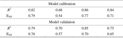
for surface runoff and sediment yield is given in Table 3. The resulting statistics for the four small DRC subcatchments all met the satisfactory criteria, and several of the statistics exceeded the good or very good criteria, as suggested by Moriasi et al.[60] Furthermore, the high R2 values indicate that there is a strong correlation between the observed and simulated surface runoff and sediment yield levels, while the ENS values show that the observed
Table 3 Model performance evaluation statistics for subcatchments
Surface runoff
Parameter Subcatchment-25 Subcatchment-27 Subcatchment-31 Subcatchment-32 Model calibration
R2 0.84 0.91 0.84 0.72
ENS 0.81 0.85 0.78 0.67
Model validation
R2 0.81 0.67 0.85 0.75
ENS 0.78 0.65 0.82 0.60
Sediment yield
Parameter Subcatchment-25 Subcatchment-27 Subcatchment-31 Subcatchment-32 Model calibration
R2 0.82 0.68 0.86 0.84
ENS 0.79 0.54 0.77 0.71
Model validation
R2 0.79 0.70 0.85 0.75
ENS 0.76 0.57 0.70 0.65
The erratic and intensive nature of rainfall has a profound impact on the generation of several peak runoff events during the monsoon (rainy) season which leads to severe soil erosion on steep sloped areas of the DRC. It was observed that 63% of annual rainfall occurred in the monsoon season (June to September). In SWAT, the erosive impact of rainfall is generally estimated in term of peak runoff generation, so the results obtained during calibration and validation are represented in Figures 8-11 for surface runoff and sediment yield for all four subcatchments. The analysis was performed for each total rainfall event and the respective total surface runoff and sediment yield generated by each event.
The overall statistical results indicated that the performance of SWAT was satisfactory for all of the subcatchments and showed the simulated values generally matched the corresponding observed values well. However, model adequacy should be further
evaluated by how well the model captures high and low rainfall events, specifically regarding the replication of fluctuations in the resulting hydrographs and sediment yields. The graphical results (Figures 8-11) revealed that SWAT was able to satisfactorily reproduce most of the low flow and sediment yield events (due to low rainfall events) although some relatively low sediment yields were considerably overpredicted; e.g., sediment yield events on August 7, 2011 (Figure 8) and December 8, 2011 (Figures 9 and 11). In contrast, it was also found that SWAT typically underestimated or overestimated high flow and sediment yield events, in response to high rainfall events.
For example: (1) a maximum intensity rainstorm on July 29, 2010 resulted in overestimation of surface runoff and sediment yields for all four subcatchments, and (2) another maximum intensity rainstorm on July 29, 2009 which resulted in underestimations for subcatchment-25 (Figure 8) versus overestimations for the other subcatchments (Figures 9-11). These discrepancies may occur due to inaccuracies in observed climate, runoff and sediment data, such as some of the rainfall events not being measured properly which in turn leads to underestimations or overestimations of runoff peaks. Another possible reason could be related to short, rapid rainfall events, which can lead to an overestimation discrepancy because small subcatchments have low times of concentration and thus a low capacity to minimize peak runoff. Also the curve number (CN) technique cannot accurately predict runoff for days that experience several storms. The underestimation and/or overestimation of sediment yield was also observed during high intensity rainstorm events which may be due to uncertainties in runoff simulation measurements as well as uncertainties in model parameterization. This may be also due to observed data used for model calibration and validation. Relatively short term events with several storms having high intensity may be not captured well by sampling of sediment data, including inaccurately high loads measured during short term events which leads to an overestimation in sediment yield.
a. Surface runoff for the 2009 to 2010 calibration period b. Surface runoff for the 2011 validation period
a. Surface runoff for the 2009 to 2010 calibration period b. Surface runoff for the 2011 validation period
c. Sediment yield for the 2009 to 2010 calibration period d. Sediment yield for the 2011 validation period Figure 9 Simulated versus observed results for subcatchment-27
a. Surface runoff for the 2009 to 2010 calibration period b. Surface runoff for the 2011 validation period
a. Surface runoff for the 2009 to 2010 calibration period b. Surface runoff for the 2011 validation period
c. Sediment yield for the 2009 to 2010 calibration period d. Sediment yield for the 2011 validation period Figure 11 Simulated versus observed results for subcatchment-32
5.1 Additional analyses of specific rainfall storm events
The detailed description of runoff generation and soil loss (sediment yield) versus the corresponding erosive events are given in Table 4 for the calibration and validation periods. It was observed that rainfall-runoff events occurred from April to September. Subcatchments-25 and -31 are natural gully systems with no engineering or vegetation protection provided by the farmers against surface runoff and soil erosion. As a result, the entire respective catchment contributed to runoff and soil erosion during most of the storms. In contrast, only the lower part of the catchments contributed to surface runoff and sediment yield in subcatchments-27 and -32 due to the terraced systems in
combination with modified gentle slopes. The cumulative rainfall of 928.3 mm during the calibration period produced a total surface runoff and sediment yield of 225 mm and 44.33 t/hm2 for subcatchment-25 (Figure 8). However, the same rainfall amount for subcatchment-27 resulted in much less total surface runoff and sediment yield of 159 mm and 8.77 t/hm2 (Figure 9), due to the terrace system that was installed in subcatchment-27. Similarly, the total rainfall of 808.06 mm during the calibration period generated overall surface runoff and sediment yields of 159.77 mm and 51.02 t/hm2 for subcatchment-31 (Figure 10), versus surface runoff and sediment yields of 54.58 mm runoff and 13.89 t/hm2 for subcatchment-32 (Figure 11).
Table 4 Total surface runoff and sediment yields corresponding to erosive rainfall events
No. of erosive rainstorm events Total rainfall/mm Total runoff and range/mm Total sediment yield and range/t·hm−2 Subcatchment-25
Calibration period 11 in 2009 400 95.5 (0.240-6.200) 13.2 (0.003-6.900)
13 in 2010 528.3 129.5 (0.310-31.500) 31.1 (0.016-9.040)
Validation period 12 in 2011 262 28.3 (0.240-7.500) 2.6 (0.008-1.100)
Subcatchment-27
Calibration period 11 in 2009 400 54.0 (0.340-18.600) 1.9 (0.001-1.100)
13 in 2010 528.3 105.2 (1.000-31.800) 6.9 (0.063-3.700)
Validation period 12 in 2011 262 23.6 (0.480-11.200) 0.52 (0.023-0.130)
Subcatchment-31
Calibration period 8 in 2009 230.8 49.3 (1.700-16.200) 20.6 (0.010-9.400)
17 in 2010 577.3 110.4 (0.400-21.200) 30.4 (0.016-9.040)
Validation period 15 in 2011 403.9 82.8 (0.710-27.300) 17.7 (0.019-5.800)
Subcatchment-32
Calibration period 8 in 2009 230.8 10.2 (0.280-3.700) 3.8 (0.045-3.200)
17 in 2010 577.3 44.4 (0.094-12.800) 10.1 (0.033-4.300)
During the analysis, it was observed that the maximum rainstorm events occurred in July and August which in turn resulted in peak surface runoff and maximum sediment yields. Therefore, the impact of maximum intensity rainstorms on surface runoff and sediment yield was also analyzed (Table 5). For subcatchments-25 and -27, the maximum intensity rainstorm occurred on July 29 in both 2009 and 2010. The maximum 30 minute-intensity (I30) of 84.3 mm/h on July 29, 2009 produced peak surface runoff and sediment yield amounts of: (1) 46.2 mm and 6.9 t/hm2 for subcatchment-25, and (2) 18.36 mm and 1.1 t/hm2 for subcatchment-27.
On July 29, 2010, the maximum intensity storm of 64.1 mm/h generated 25.9 mm/31.8 mm surface runoff and 7.8 t/hm2/1.4 t/hm2
sediment yield for subcatchments-25/-27, respectively (Figures 8 and 9). These sediment yield results again reflect the effects of the terraces installed in subcatchment-27. The maximum intensity storm that occurred on August 12, 2011 generated the lowest total rainfall (39.6 mm), and resulted in correspondingly low peak surface runoff (7.5 mm and 3.4 mm) and sediment yields (0.6 t/hm2
and 0.06 t/hm2) for subcatchments-25 and -27 (Table 5), as
compared to the impacts of the storms that occurred on July 29 during the previous two years during the calibration period.
Table 5 Peak surface runoff and sediment yield amounts for high intensity storms recorded during the calibration and
validation periods
Subcatchment Date
Total rainfall
/mm
Maximum 30 minute intensity
/mm·h-1
Peak surface runoff/mm
Sediment yield /t·hm-2
25 July 29, 2009 108 84.3 46.2 6.9
27 July 29, 2009 108 84.3 18.4 1.1
25 July 29, 2010 122.3 64.1 25.9 7.8 27 July 29, 2010 122.3 64.1 31.8 1.4 25 August 12, 2011 39.6 41.7 7.5 0.6 27 August 12, 2011 39.6 41.7 3.4 0.06 31 July 29, 2009 55.6 108.2 18.2 9.3 32 July 29, 2009 55.6 108.2 5.2 3.2 31 July 29, 2010 97.8 55.4 14.8 5.6
32 July 29, 2010 97.8 55.4 4.6 1.3
31 August 12, 2011 82.8 84.8 27.3 8.4 32 August 12, 2011 82.8 84.8 15.9 4.3 Maximum intensity rainstorm events were recorded on the same dates for subcatchments-31 and -32, but the rainfall totals and maximum 30-minute intensity levels were substantially different
than those found for subcatchments-25 and -27 (Table 5). The highest peak surface runoff and sediment yield amounts that occurred in response to the storm event on August 12, 2011 for subcatchments-31/-32 resulted in surface runoff levels of 27.3 mm/15.9 mm and sediment yields of 8.4 t/hm2/4.3 t/hm2, respectively. The results of the three storms reported for subcatchments-31 and -32 (Table 5) further confirm the effectiveness of terraces, which are installed in subcatchment-32, in reducing surface runoff and sediment yield.
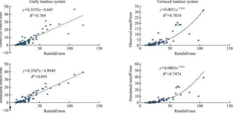
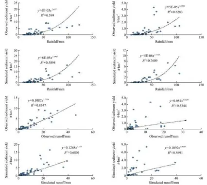
The best fit correlations between the three components of rainfall, runoff and sediment yield for the gully subcatchments and terraced subcatchments were determined separately as shown in Figure 12 using observed and simulated results. The correspondence of rainfall-runoff hydrographs with sediment yield is an indication of SWAT’s capability to simulate the hydrological regime of the DRC subcatchments. A linear correlation was the best fit between rainfall versus both the observed and simulated runoff, resulting in respective R2 values of 0.76 and 0.89, for the
gully subcatchments. However, a power correlation was determined between rainfall versus observed sediment yield (R2 = 0.59) and rainfall versus simulated sediment yield (R2=0.58) as shown in Figure 12. Likewise, power relationships between rainfall and runoff, and rainfall and sediment yield, were found to result in the strongest correlations for the terraced subcatchments, resulting in R2 values from to 0.63 to 0.76. Based on this correlation technique, the basic regression equations were developed for the DRC gully subcatchments and terraced subcatchments are as follows:
For gully subcatchments:
Runoffmm=0.358(Rainfallmm)–4.99; R2=0.89 (4)
S.Yt/hm2=0.108(Runoffmm)
1.23
; R2=0.83 (5) S.Yt/hm2=6×10-5(Rainfallmm)2.65; R2=0.59 (6)
For terraced subcatchments: Runoffmm=0.0003 (Rainfallmm)
2.58
; R2=0.74 (7) S.Yt/hm2=0.109(Runoffmm)0.90; R2=0.56 (8)
S.Yt/hm2=5×10-6(Rainfallmm)3.11; R2=0.76 (9)
Figure 12 Correlation between rainfall, runoff and sediment yield for the gully/ terraced subcatchments, for both the observed and simulated data
6 Conclusions and recommendations
In this research, the SWAT model was applied on a daily time step and was used to simulate soil erosion for specific storm events for four small DRC subcatchments. Subcatchments-25 and -31 were characterized by incised gullies while subcatchments-27 and -32 consist of terraced landuse systems. The performance of the SWAT model was satisfactory with R2 values ≥0.67 and ENS ≥0.53
for both surface runoff and sediment yield during the calibration (2009-2010) and validation (2011) periods. The PUSLE factor was
found to be the most sensitive factor during model calibration. It was observed that all of the rainfall-runoff events occurred during the monsoon season (June to September).
It was estimated that in 2009, the gully subcatchments produced annual sediment yield that ranged from 13.19 t/hm2 to 20.60 t/hm2 in response to rainfall events that were between 230.76-399.95 mm and surface runoff amounts that ranged from 49.34 mm to 95.59 mm. In comparison, the terraced subcatchments produced 1.90-3.77 t/hm2 sediment yield for the same rainfall levels and surface runoff that was measured from 10.17 mm to 54.0 mm. In 2010, the annual sediment yield for the gully subcatchments was observed to be 30.41-31.12 t/hm2, due to rainfall levels of 528.29-577.30 mm that produced surface runoff amounts of 110.43-129.53 mm. In contrast, it was observed that the terraced subcatchments yielded 0.87-10.11 t/hm2 of sediment annually, in response to rainfall amounts of 432.3-577.30 mm that
resulted in surface runoff that ranged from 44.4 mm to 110.43 mm. 2011 was an interesting climate year of reference, because it was relatively dry year which resulted in rainfall amounts that ranged from 261.6 mm to 403.88 mm for the gully subcatchments and 194.8 mm to 403.88 mm for the terraced subcatchments. As a result, surface runoff of 28.34-82.84 mm and sediment yield of 2.59-17.73 t/hm2 occurred for the gully subcatchments while the terraced catchments produced runoff of 23.61-30.47 mm and corresponding sediment yield levels of 0.52-4.19 t/hm2. It was found that the sediment yield generated by the terraced subcatchments was 4-5 times lower than the sediment yields that were exported from the gully subcatchments. Thus, there is a huge potential for terraces to reduce the soil erosion in the DRC. It is recommended that the model application should be extended for larger catchments located within the Pothwar area, to identify efficient locations for soil and water conservation structures and management practices.
Acknowledgments
assistance of Dr. Philip W. Gassman (Section Editor of IJABE) and the reviewers.
Appendix A. Additional photos of structural
conservation practices used in the Pothwar region of
Pakistan
[63]Figure A1 Terraced cultivated lands in Pothwar
Figure A2 Breached terrace bund/embankment
Figure A3 Loose stone structures system
Figure A4 Loose stone structure in the field
Figure A5 Front view of conservation structure built using local available stones
[References]
[1] Lal R. Soil Erosion and the global carbon budget. Environ. Intern., 2003; 29(4): 437-450.
[2] Chen J, Chen J, Tan M, Gao Z. Soil degradation: A global problem endangering sustainable development. J. Geogr. Sci., 2002; 12(2): 243-252.
[3] Govers G, Merckx R, van Wesemael B, van Oost K. Soil conservation in the 21st century: Why we need smart agricultural intensification. Soil, 2017; 3: 45–59.
[4] FAO and ITPS. Status of the world’s soil resources (SWSR); Main Report; Food and Agriculture Organization of the United Nations and Intergovernmental Technical Panel on Soils: Rome, Italy, 2015. 608 p. [5] Borrelli P, Robinson D, Fleischer L R, Lugato E, Panagos P. An
assessment of the global impact of 21st century landuse change on soil erosion. Nature Communications, 2017; 8(1).
[6] Young A M, Land degradation in south Asia: its severity, causes and effects upon the people. World Soil Resources Reports, 1994; 78: 75p. FAO, Rome, Italy.
[7] Scherr S J, Yadav S. Land degradation in the developing world: Implications for food, agriculture and the environment to 2020. Food, Agriculture and the Environment Discussion Paper 14. International Food Policy Research Institute (IFPRI), Washington, DC, U.S.A. 1996. [8] Oldeman L R, Hakkeling R T A, Sombroek W G. World map of status of
human-induced soil degradation, with explanatory note (second revised edition). International Soil Reference and Information Centre (ISRIC), Wageningen, UNEP, Nairobi, 1991.
[9] Montgomery D R. Soil erosion and agricultural sustainability. P. Natl. Acad. Sci. USA, 2007; 104(33): 13268–13272.
[10] Vanacker V, von Blanckenburg F, Govers G, Molina A, Poesen J, Deckers J, et al. Restoring dense vegetation can slow mountain erosion to near natural benchmark levels. Geology, 2007; 35(4): 303–306.
[11] Pimentel D, Nadia K. Ecology of soil erosion in ecosystems. Ecosystems, 1998; 1(5): 416–426.
[12] Pimentel D. Soil erosion: A food and environmental threat. Environment, Development and Sustainability, 2006; 8(1): 119–137. [13] Nasir A, Uchida K, Ashraf M. Estimation of soil erosion by using
RUSLE and GIS for small mountainous watersheds in Pakistan. Pakistan Journal of Water Resources, 2006; 10(1): 11–21.
[14] Ashraf M, Hassan F U, Saleem A, Iqbal M M. Soil conservation and management: A prerequisite for sustainable agriculture in pothwar. Science, Technology and Development, 2002; 21(1): 25–31.
[15] Oweis T, Ashraf M. Assessment and options for improved productivity and sustainability of natural resources in Dhrabi watershed Pakistan. ICARDA, 2012; xviii + 205: p77. Aleppo, Syria.
[16] Ghulam N, Latif M, Ahsan M, Anwar S. Soil erosion estimation of Soan river catchment using remote sensing and geographic information system. Soil and Environment, 2008; 27(1): 36–42.
[17] Renard K G, Ferreira V A. RUSLE model description and database sensitivity. J Environ Qual, 1993; 22:458–466.
[18] Flanagan D C, Gilley J E, Franti T G. Water erosion prediction project (WEPP): Development history, model capabilities and future enhancements. Trans ASABE, 2007; 50(5): 1603–1612.
[19] Foster G R, Lane L J. User requirements: USDA water erosion prediction project (WEPP). NSERL Report No. 1, USDA ARS National Soil Erosion Research Laboratory, West Lafayette, Indiana, 1987. 43 p. [20] Klik A, Rattanaareekul W, Bushsbaum T. Chapter 5: soil erosion
Natural Resources in Dhrabi Watershed Pakistan Aleppo, Syria: International Center for Agricultural Research in the Dry Areas (ICARDA). 2012; pp.125–194.
[21] Verstraeten G, Poesen J, de Vente J, Koninckx X. Sediment yield variability in Spain: A quantitative and semi-qualitative analysis using reservoir sedimentation rates. Geomorphology, 2003; 50(4): 327–348. [22] Pimentel D, Burgess M. Soil erosion threatens food production.
Agriculture, 2013; 3(3): 443–463.
[23] Ghafari H, Gorji M, Arabkhedri M, Roshani G A, Heidari A, Akhavan S. Identification and prioritization of critical erosion areas based on onsite and offsite effects. Catena, 2017; 156: 1–9.
[24] Wischmeier W H, Smith D D. Predicting rainfall erosion losses-a guide to conservation planning. Agriculture Handbook No. 537, USDA, Washington, 1978; 58p.
[25] Arnold J G, Srinivasan R, Muttiah R S, Williams J R. Large area hydrologic modeling and assessment: Part I. Model Development. Journal of the American Water Resources Association, 1998; 34(1): 73-89. [26] Williams J R, Berndt H D. Sediment yield prediction based on watershed
hydrology. Trans ASAE, 1977; 20(6): 1100–1104.
[27] Borah D K, Bera M. Watershed-scale hydrologic and nonpoint-source pollution models: Review of mathematical bases. Trans. ASAE, 2003; 46(6): 1553–1566.
[28] Arnold J G, Fohrer N. SWAT2000: Current capabilities and research opportunities in applied watershed modelling. Hydrological Processes, 2005; 19(3): 563–572.
[29] Tripathi M P, Panda R K, Raghuwanshi N S. Identification and prioritisation of critical sub watersheds for soil conservation management using the SWAT Model. Bio Systems Engineering, 2003; 85(3): 365–379.
[30] Zabaleta A, Meaurio M, Ruiz E, Antigüedad I. Simulation climate change impact on runoff and sediment yield in a small watershed in the Basque Country, northern Spain. Journal of Environmental Quality, 2014; 43(1): 235–245.
[31] Lemann T, Zeleke G, Amsler C, Giovanoli L, Suter H, Roth V. Modelling the effect of soil and water conservation on discharge and sediment yield in the upper Blue Nile Basin, Ethiopia. Applied Geography, 2016; 73: 89–101.
[32] Roth V, Lemann T. Comparing CFSR and conventional weather data for discharge and soil loss modelling with SWAT in small catchments in the Ethiopian highlands. Hydrology and Earth System Sciences, 2016; 20 (2): 921–934.
[33] Setegn S G, Dargahi B, Srinivasan R, Melesse A M. modeling of sediment yield from Anjeni-Gauged watershed, Ethiopia using SWAT Model. Journal of the American Water Resource Association, 2010; 46(3): 514–526.
[34] Gassman P W, Reyes M R, Green C H, Arnold J G. The soil and water assessment tool: Historical development, applications, and future research directions. Transactions of the ASABE, 2007; 50(4): 1211–1250. [35] Gassman P W, Sadeghi A M, Srinivasan R. Applications of the SWAT
model special section: Overview and insights. J Environ Qual, 2014; 43(1): 1–8.
[36] Douglas-Mankin K R, Srinivasan R, Arnold J G. Soil and Water Assessment Tool (SWAT) Model: Current developments and applications. Trans ASABE, 2010; 53(5): 1423–1431.
[37] Tuppad P, Douglas-Mankin K R, Lee T, Srinivasan R, Arnold J G. Soil and Water Assessment Tool (SWAT) Hydrologic/ water quality model: extended capability and wider adoption. Trans ASABE, 2011; 54(5): 1677–1684.
[38] Krysanova V, White M. Advances in water resources assessment with SWAT-An overview. Hydrol Sci J, 2015; 60(5): 771–783.
[39] Bressiani D A, Gassman P W, Fernandes J G, Garbossa L H P, Srinivasan R, Bonuma´ N B, Mendiondo E M. A review of SWAT (soil and water application tool) applications in Brazil: Challenges and prospects. Int J Agric Biol Eng, 2015; 8(3): 9–35.
[40] Mosbahi M, Benabdallah S, Boussema M R. Assessment of soil erosion risk using SWAT Model. Arab J Geosci, 2013; 6(10): 4011–4019.
[41] CARD. SWAT literature database for peer-reviewed journal articles. Center for Agricultural and Rural Development, Iowa State University, Ames, Iowa, 2018.
[42] Samad N, Chauhdry M H, Ashraf M, Saleem M, Hamid Q, Babar U, et al. Sediment yield assessment and identification of dam sites for rawal dam catchment. Arab J Geosci, 2016; 9: 466.
[43] Ghoraba S M. Hydrological modeling of the Simly Dam Watershed (Pakistan) using GIS and SWAT Model. Alexandria Engineering Journal, 2015; 54(3): 583–594.
[44] Bailey T C, Gatrell A C. Interactive spatial data analysis. Harlow: Longman, 1995.
[45] Wong D W S. Interpolation: Inverse-Distance Weighting. In: The International Encyclopedia of Geography, 2017.
[46] Google Earth. Mountain view, CA. https://www.google.com/earth/. Accessed on [2018-11-30]
[47] Soil & Water Conservation Research Institute. Chakwal: Under Ayub Agriculture Research Institute (AARI), Faisalabad. Government of Punjab, Pakistan.
[48] Iqbal M N, Oweis T Y, Ashraf M, Bashir H, Majid A. Impact of land-use practices on sediment yield in the Dhrabi Watershed of Pakistan. Journal of Environmental Science and Engineering A1, 2012; 406–420.
[49] Neitsch S L, Arnold J G, Kiniry J R, Williams J R. Soil and water assessment tool, theoretical documentation - Version 2009. Grassland, Soil and Water Research Laboratory – Agricultural Research Service Blackland Research Center – Texas, 2011.
[50] SWAT (Soil and Water Assessment Tool). http://swat.tamu.edu/software/arcswat/. Accessed on [2018-11-30] [51] Olivera F, Valenzuela M, Srinivasan R, Choi J, Cho H, Koka S, et al.
ARCGIS-SWAT: A geodata model and GIS interface for SWAT. Journal of the American Water Resources Association, 2006; 42(2): 295–309. [52] Soil Conservation Service. Section 4 hydrology In: National Engineering
Handbook. U.S. Department of Agriculture-Soil Conservation Service, Washington, D.C, 1972.
[53] Green W H, Ampt G A. Studies on soil physics, 1. The flow of air and water through soils. Journal of Agricultural Sciences, 1911; 4: 11–24. [54] Her Y, Frankenberger J, Chaubey I, Srinivasan R. Threshold effects in
hru definition of the soil and water assessment tool. Transactions of the ASABE, 2015; 58(2): 367–378.
[55] Arnold J G, Moriasi D N, Gassman P W, Abbaspour K C, White M J, Srinivasan R, et al. SWAT: Model use, calibration, and validation. Transactions of the ASABE, 2012; 55(4): 1491–-1508.
[56] Arnold J G, Youssef M A, Yen H, White M J, Sheshukov A Y, Sadeghi, A M, et al. Hydrological processes and model representation: Impact of soft data on calibration. Transactions of the ASABE, 2015; 58(6): 1637–1660.
[57] Engel B, Storm D, White M, Arnold J, Arabi M. A hydrologic/water quality model application protocol. J. American Water Resour. Assoc., 2007; 43(5): 1223–1236.
[58] Santhi C, Arnold J G, Williams J R, Dugas W A, Srinivasan R, Hauck L M. Validation of the SWAT Model on a large river basin with point and nonpoint sources. J. American Water Resour. Assoc., 2001; 37(5): 1169–1188.
[59] Krause P, Boyle D P, Bäse F. Comparison of different efficiency criteria for hydrological model assessment. Advances in Geosciences, 2005; 5: 89–97.
[60] Moriasi D N, Gitau M W, Pai N, Daggupati P. Hydrologic and water quality models: Performance measures and evaluation criteria. Trans. ASABE, 2015; 58(6): 1763–1785.
[61] Nash J, Sutcliffe J. River flow forecasting through conceptual models: Part I. A Discussion of Principles. J. Hydrol., 1970; 10(3): 282–290. [62] Stigler S M. Francis Galton’s account of the invention of correlation.
Statistical Science, 1989; 4(2): 73–79.


![Table 2 Soil erosion parameter ranking used for model calibration[63]](https://thumb-us.123doks.com/thumbv2/123dok_us/593251.2058568/6.595.308.554.581.683/table-soil-erosion-parameter-ranking-used-model-calibration.webp)