Development of deficit irrigation for maize crop under drip
irrigation in samaru-nigeria
Oiganji Ezekiel
1*, H. E. Igbadun
2, O. J. Mudiare
2, M. A. Oyebode
2(1. Department of Crop Production Technology, Federal College of Forestry, Forestry Research Institute of Nigeria, Jos- Nigeria; 2. Department of Agricultural Engineering, Ahmadu Bello University, Zaria, Nigeria)
Abstract: In the past, outcome of any water management strategy could only be known after field experiment, in recent times, means of evaluating the implications of irrigation schedules without field experiment is fast gaining grounds with the use of models. This research work present a scenarios studies for different developed irrigation scheduling options for a drip irrigated maize crop at the Institute for Agricultural Research (IAR) irrigation farm Samaru-Nigeria during 2013 and 2014 cropping season using a computer-based model. Aqua Crop was calibrated and validated with data obtained from the field, it was further used to generate scenario of different irrigation scheduling outcome. Grain and biomass yields, harvest index, seasonal evapotranspiration and crop water productivity were determined. The general trend of the results suggests that skipping regular irrigations may be advantageous if such is done at grain-filling stage, though most of the time this stage is intercepted by rain in the study area. The scenario studies showed that the peak grain and biomass yield value of 3273 and 10492 kg ha-1 was recorded when 20 mm water application depth (WAD) with 3-day irrigation interval applied across all the
growth stages; the irrigation water productivity with respect to grain and biomass yield were 0.83and 2.65 kg m-3 respectively.
The possible consequences of a developed irrigation scheduling on the crop and its environment, could be analysed without necessarily going to the field. The Aqua Crop model is useful for on-the-desk assessing of the impact of irrigation schedulling protocols.
Keywords: Aqua Crop model, calibration, validation, irrigation schedulling, Water productivity
Citation: Ezekiel O., H. E. Igbadun, O. J. Mudiare, and M. A. Oyebode. 2017. Development of deficit irrigation for maize crop under drip irrigation in samaru-nigeria. Agricultural Engineering International: CIGR Journal, 19(1): 94–107.
1 Introduction
The emerging threat to sustainability of agriculture globally requires a paradigm shift in the way irrigation is practiced; the rapid increase of the world population and the corresponding demand for extra water by water users forces the agricultural sector to use its irrigation water more efficiently (Andarzian et al., 2011). This entails adoption of irrigation water management strategy that can facilitate the achievement of the goal of producing more crops per drop of water, which is the use of drip irrigation system and adoption of deficit irrigation scheduling
Received date: 2016-03-22 Accepted date: 2017-01-07
* Corresponding author: Oiganji Ezekiel, Department of Crop Production Technology, Federal College of Forestry, Forestry Research Institute of Nigeria, Jos- Nigeria. Tel: +2348061279887. Email: ezeganji@gmail.com.
among others (Molden et al., 2003; Kendall, 2011; Igbadun et al., 2012).
Drip irrigation system is one of the fastest expanding technologies in modern irrigated agriculture with great potential for achieving high effectiveness of water-use. It allows judicious use of water and fertilizer during irrigation of a wide range of crops (Segal et al., 2000; Mofoke et al., 2006; Oyebode et al., 2011). Deficit irrigation schedulling has been recognized as a viable practice that could lead to increased crop yield, reduced
negative environmental impact and improved
2009; Himanshu et al., 2012).
Evaluation of irrigation scheduling methods can be carried out directly by conducting field trials. However, this approach is always expensive, time consuming, subject to uncontrolled environmental condition and practically difficult for farmers to analyse long-term effects and large impact scenarios beyond experimental sites and years. An easier option is to use crop simulation models for the exercise (Igbadun, 2008). Crop simulation models are computer software describing the dynamics of the growth of a crop in relation to the environment (Kumar and Ahlamat, 2004; Oguntunde, 2004; Abedinpour et al., 2012).
Research outcome documented on deficit irrigation schedulling are very few in the sub-Saharan African countries and for Samaru-Nigeria in particular. Igbadun (2012) for instance, reported field experiments on the impacts of methods of administering growth-stage deficit irrigation on yield and soil water balance of a maize crop in Samaru. Other investigators (Halilu, 2014; Ismail, 2014) worked on water use for vegetable crops of watermelon and tomatoes in Samaru and Kadawa, Nigeria. Thus, knowledge gaps remain as to the growth stage deficit irrigation tolerance limit for maize crop under different soil types, climatic conditions, different methods of administering deficit irrigation and the corresponding impacts on yield, soil water balance and water productivity. If a field study is to be done to answer this question, it will take several years and a high cost with several uncertainties (Igbadun, 2008). This suggests that more research work that could be applied beyond years, site and climatic conditions is needed; which can only be possible through the instrumentality of a model, and hence, Aqua Crop model for simulation of scenarios was adopted, though not new, but yet to be explored by irrigators and researchers in the study area. The outcome of such evaluations will constitute a body of knowledge that can be used to advise and help farmers plan for their expected returns, help projects managers, consultants, irrigation engineers and agronomists to increase crop water productivity and optimal water management decision (Kirnak and Demirtas, 2006).
In the case of maize, many models have been tested:
for example, the Cropsyst which is based on both water and solar radiation driven modules, WOFOST which simulates crop growth using a carbon driven approach, amongst others are Ceres, CERES-Maize, Hybrid-Maize and EPIC model (Tanner and Sinclair, 1983; Jones and Kiniry, 1986; Azam et al., 1994; Cavero et al., 2000; Steduto, 2003; Stockle et al., 2003; Steduto and Albrizio, 2005; Steduto et al., 2007; Yang et al., 2004; Heng et al., 2009). They differ among themselves, and are able to simulate plant production with higher or lower degree of accuracy. Most of the models require advanced modelling skills for their calibration and require large number of model input parameters. Efforts to achieve a new model that is less complex with accuracy, simplicity and versality with fewer numbers of inputs have been made. An outcome of such efforts is the AquaCrop model which focuses on yield response to water (Steduto et al., 2009). The FAO crop model, AquaCrop, simulates attainable yields of major herbaceous crops as a function of water consumption under rainfed, supplemental, deficit and full irrigation conditions (Yang et al., 2004; Steduto and Albrizio, 2005; Ma et al., 2007; Steduto et al., 2007; Lopez-Cedron, 2008; Heng et al., 2009). For a more detailed description of the model of the principles and operations see Steduto et al. (2009) and Raes et al. (2009). The ability of AquaCrop to simulate yields for different crops has been extensively tested by several researchers around the globe in diverse environments and all have reported positive results, such as: barley( Araya et al., 2010a), teff (Araya et al., 2010b), cotton (Baumhardt et al., 2009; Hussein et al., 2011), quinoa (Geerts et al., 2009), maize (Heng et al., 2009; Hsiao et al., 2009; Zinyengere et al., 2011), potato (Vanuytrecht et al., 2011) , wheat (Andarzian et al., 2011) and canola ( Zeleke et al., 2011).
the site, years and climatic condition. As such, the aim of this paper was to develop deficit irrigation schedulling strategies, and applying it for simulating the effects different irrigation scenarios for a maize crop under gravity-drip irrigation in Samaru Nigeria during 2013 and 2014 cropping season.
2 Materials and methods
2.1 Study area
The field experiments used in calibrating and
validating the Aqua Crop model were carried out at the Institute for Agricultural Research (IAR) Irrigation farm, Ahmadu Bello University, Zaria, Nigeria. Zaria lies on 11°11′N and 7°38′E, and at an altitude of 686 m above mean sea level, within the Northern Guinea Savannah ecological zone (Odunze, 1998). The weather data for the crop growing seasons are presented in Table 1 obtained from the meteorological station at the IAR farm; while the mean characteristics of the soils of the study location A and B is shown in Table 2.
Table 1 Average weather data for the 2013/2014 crop growing season
Months Humidity, % Max. temp., °C Min. temp., °C Sunshine, h Wind speed, km d-1 EToa, mm d-1 Total rainfall, mm
January 19.37 32.48 17.74 8.01 142.66 6.82 -
February 13.52 35.50 18.79 7.49 131.44 8.56 0.4
March 26.37 39.29 22.77 7.63 118.24 9.14 15.74
April 38.85 37.47 24.77 7.09 143.03 7.89 14.76
Note: EToa = Reference evapotranspiration.
Table 2 Physical properties of soils at various depths at the irrigation research farm, Samaru
Depth, mm FC, %Vol
PWP, %Vol
Bulk density, g cm-3
Hydraulic conductivity, mm hr-1
TAW, mm m-1
Ksat,
mm day-1 Clay, % Silt, % Sand,% Texture classa
0-150 24.8 13.6 1.58 70 112 70 22 28 50 Loam
150-300 26.3 15.9 1.58 100 104 100 26 22 54 Loam
300-450 27.4 17.1 1.57 100 103 100 28 18 54 Loam
450-600 25.9 15.9 1.58 125 100 125 26 18 56 Sandy clay loam
600-800 29.5 18.2 1.55 125 113 125 30 22 48 Sandy clay loam
Note: Texture classa (Odunze, 1998).
2.2 Experimental layout and agronomic practices
Two field experiments were carried out during the 2013 and 2014 irrigation season for the purpose of generating data for calibrating and validating the Aqua Crop model. The size of the experimental field in each season was 0.2 ha, the distance between field A and B was 4 m. Each field was divided into plot sizes of 5 m by 1.8 m each. Each plot consisted of three drip lines spaced 0.6 m apart. SAMMAZ 14 maize variety was planted on the 7th February 2013 in the first season and 6th February
2014 in the second season.
In both seasons the planting was done along the drip lines, a plant spacing of 30 cm between plants and 60 cm between rows. Each field experiment consisted of eight treatments replicated three times and laid in a randomized complete block design, across the general slope of the field in order to ensure as much homogenous soil conditions as possible within the blocks. The treatments
were based on water application regulated at selected crop growth stages. The description of the experimental treatments is presented in Tables 3 and 4.
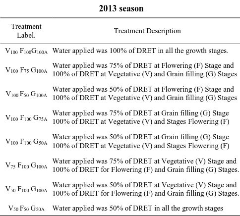
Table 3 Description of experimental treatments for Field A in
2013 season
Treatment
Label. Treatment Description
V100 F100G100A Water applied was 100% of DRET in all the growth stages.
V100 F75 G100A
Water applied was 75% of DRET at Flowering (F) Stage and 100% of DRET at Vegetative (V) and Grain filling (G) Stages
V100 F50 G100A Water applied was 50% of DRET at Flowering (F) Stage and
100% of DRET at Vegetative (V) and Grain filling (G) Stages
V100 F100 G75A Water applied was 75% of DRET at Grain filling (G) Stage
100% of DRET at Vegetative (V) and Stages Flowering (F)
V100 F100 G50A Water applied was 50% of DRET at Grain filling (G) Stage
100% of DRET at Vegetative (V) and Stages Flowering (F)
V75 F100 G100A Water applied was 75% of DRET at Vegetative (V) Stage and
100% of DRET for Flowering (F) and Grain filling (G) Stages.
V50 F100 G100A
Water applied was 50% of DRET at Vegetative (V) Stage and 100% of DRET for Flowering (F) and Grain filling (G) Stages.
V50 F50 G50A Water applied was 50% of DRET in all the growth stages
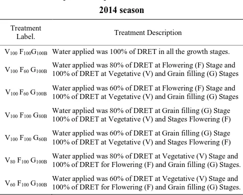
Table 4 Description of experimental treatments for Field B in
2014 season
Treatment
Label. Treatment Description
V100 F100G100B Water applied was 100% of DRET in all the growth stages.
V100 F60 G100B
Water applied was 80% of DRET at Flowering (F) Stage and 100% of DRET at Vegetative (V) and Grain filling (G) Stages
V100 F60 G100B
Water applied was 60% of DRET at Flowering (F) Stage and 100% of DRET at Vegetative (V) and Grain filling (G) Stages
V100 F100 G80B
Water applied was 80% of DRET at Grain filling (G) Stage 100% of DRET at Vegetative (V) and Stages Flowering (F)
V100 F100 G60B
Water applied was 60% of DRET at Grain filling (G) Stage 100% of DRET at Vegetative (V) and Stages Flowering (F)
V80 F100 G100B
Water applied was 80% of DRET at Vegetative (V) Stage and 100% of DRET for Flowering (F) and Grain filling (G) Stages.
V60 F100 G100B
Water applied was 60% of DRET at Vegetative (V) Stage and 100% of DRET for Flowering (F) and Grain filling (G) Stages.
Note: DRET= Daily Reference Evapotranspiration.
In 2013 season, manual weeding with the use of hoe was carried out three times for both fields at three, six and nine weeks after planting. In 2014 season, however, weeding was carried out thrice at two, five and nine weeks after planting since weed proliferation on the experimental field was more.
Compound fertilizer Nitrogen Phosphorus and potassium (NPK) 15:15:15 was applied at the rate of 60 kg N ha-1 at three weeks after planting, applied as
basal dose. Urea fertilizer was used for top dressing at six weeks after planting at a rate of 60 kg N ha-1 as
recommended by Igbadun (2012) thus the total N applied was 120 kg ha-1. The fertilizers were applied after
weeding on each occasion. There was no incidence of pests or diseases during the 2012/2013 cropping season. In 2013/2014 cropping season however, there was attack of aphids during the 5th week, which was managed with
the application of karate at 0.8 L ha-1 using 40 mL in 15 L
knapsack sprayer as recommended by Avav and Ayuba (2006). The following growth-stages ranges were adopted in this research as reported by Igbadun (2012): Vegetative (15-42DAP); Flowering – tasseling to silking (43- 63 DAP) and grain filling to physiological maturity stages (64-95 DAP). Date of sowing and date of emergence were recorded. Emergence date was considered when 90% of seedlings had emerged. Flowering and duration of flowering, maximum canopy cover, senescence and maturity observations were also made.
2.3 Soil water balance
The water balance is an accounting of the inputs and
outputs of water which can be determined by calculating the input, output and storage changes of water at an agricultural land. It can be by is expressed as (Allen et al., 1998; Abedinpour et al., 2012):
I+R=ET+Rf+intL+DP±ΔS (1)
where, Äs = difference between soil moisture content at the beginning and end of the season, mm; ET = seasonal evapotranspiration, mm; I=seasonal irrigation depth, mm;
R = amount of rainfall, mm; Rf = amount of runoff, mm, which was zero in this experiment because water was confined within the basin; IntL=precipitation intercepted by the crop canopy, mm; DP = seasonal deep percolation depth, mm.
2.3.1 Computation of soil moisture content
Soil moisture content of the experimental plots was monitored throughout the crop growing season using calibrated gypsum blocks (227 Delmhorst; Campbell Scientific; Logan, Utah, U.S.A.) in both seasons. Four gypsum blocks were installed in each experimental plot at 12, 25, 45 and 70 cm soil profile depths to monitor soil moisture changes at 0-15, 0-30, 30-60, 60-90 cm depths. Soil moisture resistances were measured using Delmhorst soil moisture tester (FX-2000 model, Delmhorst, New York, U.S.A.), a day after every irrigation and just before the next irrigation.
The resistance measured were related to gravimetric soil moisture content using gypsum-moisture content calibration curve developed for the sets of gypsum blocks used with R2 value of 0.87. The calibration curve was
expressed as:
GMC = 44.75* R-0.24 (2)
where, GMC is the gravimetric moisture content (% dry weight basis) and R, the electrical resistance in ohm (Ω)
The actual crop evapotranspiration was calculated from the measured soil moisture content data using gypsum blocks as outlined by Michael (1978). Equation
(3) was used to estimate the actual crop
evapotranspiration (Eta)
The actual crop evapotranspiration outlined by Michael (1978) is expressed as:
1 2
1
100
n
a i i i
M M
ET D B
(3)sampling in the ith layer; M2=gravimetric moisture
content (g g-1) at the second sampling in the ith layer;
Di = depth of its layer, mm; n = number of layers within
the soil profile; Bi = apparent specific gravity of the soil
layer
2.4 Above ground biomass and final harvesting
The crop attained physiological maturity at 89 and 86 DAP in 2013 and 2014 seasons, respectively; irrigation was withdrawn thereafter to allow the crop to dry in both seasons. Harvest was done by cutting the above ground dry matter. Each plot had three rows with an area of 1.2 m × 5 m which constituted the plot for final yield assessment. They were conveyed to the laboratory for curing for three weeks until the biomass was fully dried and the maize grain had attained 13.5% moisture content on dry base. The dry matters w ere then weighed, the maize cobs threshed and weighed.
2.5 Performance evaluation of a model
Since no single measure can determine how well a simulation model performs, a combination of statistical indices are generally used to evaluate the model (Anjum et al., 2014). The agreement between the measured and the simulated values was assessed using the following statistical indices:
The RMSE gives the weighted variations in errors (residual) between the modelled and observed values and is calculated as follows (Nash and Sutcliff, 1970):
2
1
( i i)
RMSE M S
n
(4)The coefficient of Variation is a measure of variability expressed as (Willmout and Matsuura, 2005):
2
( )
1
100 * i i
i
M S
CV
n S
(5)where, Si is simulated; Mi is measured value; n is the
number of measurements.
Modelling efficiency is a measure of the degree of fit between simulated and measured data, similar to the coefficient of determination (R2), and varies from negative infinity for total lack of fit to 1 for an exact fit. The expression is given in Equation (6) (Willmott, 1982):
2 2
2
( ) ( )
( )
i m i i
i m
S S M S
EF
S S
(6)where, Sm is mean simulated values
The coefficient of residual mass is an indicator of the tendency of the model to either over-or under-predict measured values, a positive value indicates a tendency of under-prediction, while a negative value indicates a tendency of over-prediction (Igbadun, 2012; Kahimba et al., 2009).
i i
i
S M
CRM
S
(7)The model performance was further evaluated using prediction error. The expression is given in Equation 8 (Nash and Sutcliff, 1970):
100
i i
i
S M
Pe M
(8)
where all the terms are as previously defined.
2.6 Running Aqua Crop model
The input data used for the running of the model include: weather, soil, crop and irrigation schedulling (timing of irrigation and amount of water applied). The weather data were obtained from the meteorological station in the Institute for Agricultural Research Farm close to the research field, for the two seasons. Maize crop simulation parameters used for calibrating Aqua Crop Software are presented in Table 5. The hydraulic properties of the soil used as input were those of the experimental site as presented in Table 2.
2.6.1 Calibration procedure
Model calibration involves a systematic adjustment of the parameters of a model such that the model can describe more closely the system behaviour for site-specific application as reported by Igbadun (2012). During the calibration process, conservative parameters wereadapted from the report of Hsiao et al (2009), these parameters included canopy cover growth and canopy decline coefficient; crop coefficient for transpiration at full canopy; water productivity (WP); soil water depletion thresholds for inhibition of leaf growth, stomata conductance and acceleration of canopy senescence.
Table 5 Crop input parameters for Aqua Crop model
Description Value Source
Base temperature 8°C Hsiao et al., 2009
Cut-off temperature 35°C Hsiao et al., 2009
Canopy cover per seedling at 90% emergence
(CCo) 6.5 cm2 Hsiao et al., 2009 Canopy growth coefficient (CGC) 19.6% Dirk et al., 2010
Maximum canopy Cover (CCx) 60% Function of plant density
Canopy decline Coefficient (CDC) at senescence 12.5% Dirk et al., 2010
Water productivity normalized for ETo and CO2
during yield formation 85% Dirk et al., 2010
Leaf growth threshold p-upper 0.10 Hsiao et al., 2009
Leaf growth threshold p-lower 0.45 Hsiao et al., 2009
Leaf growth stress coefficient curve shape 2.9 Hsiao et al., 2009
Stomata conductance thresh p-upper 0.45 Hsiao et al., 2009
Stomata stress coefficient curve shape 6.0 Hsiao et al., 2009
Senescence stress coefficient p-upper 0.45 Hsiao et al., 2009
Senescence stress coefficient curve shape 1.5 Hsiao et al., 2009
Coefficient, inhibition of leaf growth on HI 7 Dirk et al., 2010
Coefficient, inhibition of stomata on HI 3.0 Dirk et al., 2010
Maximum basal crop coefficient (Kcb) 1.05 Allen et al., 1998
Effective rooting depth 0.6 m Keller and Bliesner, 1990 Water productivity normalized for ETo and CO2
(g m-2) 31.7 a
Plant density 55,556
plants ha-1 a
Time from sowing to emergence 8 days a
Length of the flowering stage 10days a
Time from sowing to maximum canopy cover 47days a
Time from sowing to flowering 52 days a
Time to maximum rooting depth 60 days a
Time from sowing to start Senescence 65 days a
Time from sowing to maturity 90 days a Note: a= data obtained from the field.
The days to emergence, maximum canopy, senescence and maturity as observed from the field were 8, 47, 65 and 90 days, respectively. The calibrated maximum canopy cover was 60%, values of CGC and CDC for the experiment were 19.6% and 22.5%, respectively. The following was recorded from the model output: controlled days to flowering, duration of flowering, length to building of yield, 52, 10 and 34 days, respectively. The effective rooting depth was set at 0.6 m, while the Kcbx
value obtained was 1.05 which is in line with the crop coefficients for the midseason as giving by FAO-56 (Allen et al., 1998). The value of WP adopted was 31.7 g m-2 which was in the range (31-34 g m-2)
suggested for the Aqua Crop for C4 crops (crops that
produces the 4-carbon compound oxalocethanoic acid as the first stage of photosynthesis). The harvest index obtained was 32% and the soil set as clay loam with
initial soil condition as wet dry.
Factors pertaining to expansion stress were calibrated to have the upper threshold, lower threshold and shape factors to be 0.10, 0.45 and 2.9, respectively. Also, the stomata closure stress; upper threshold and shape factor were 0.45 and 6.0, respectively, while the lower threshold was set at the permanent wilting point.
Moreover, the early senescence stress, upper threshold and shape factor were 0.45 and 1.5, respectively, while the lower threshold was set at the permanent wilting point. These calibrated coefficients were related to the crop water stress function in the Aqua Crop model, which was used to simulate the yield from the different experimental plots.
During the calibration process, the biomass and yield were compared with the measured data using water productivity and the crop coefficient. At the same time simulated irrigation water productivity was compared with the observed data in the field experiment for field B during the 2013 cropping season which was used for the calibration exercise. The process was repeated several times to list out a set of parameters that produced results in line with the measured data. The final values of the adjusted parameters at which the model simulated outputs had the highest correlation with the field-measured data were adopted as input data for the model as shown in Table 6.
Calibration was accomplished by using the observed values from the field experiment during the 2013 (field B) as model input and then using the model to predict the output. Subsequently the output values were compared with observed field data.
2.7 Calibration and validation of the Aqua Crop model
Model calibration was carried out using field data for 2013 cropping season, while model validation was carried out by comparing independent field data for 2014 cropping season and model output. Grain yield, biomass yield, Seasonal crop water use and irrigation water productivity for biomass and yield, were considered as the evaluation parameters for the Aqua Crop model. The crop parameters obtained from the calibration of the model were used in the validation of the model; details on the calibration and validation of AquaCrop model was reported by Oiganji et al. (2016).
2.8 Scenario study on deficit irrigation schedulling on yield and water productivity of maize
After the model was found to satisfactorily simulate yield and water productivity in its predictions, it was used for scenario analyses to evaluate the water management practices for drip irrigated maize in the study area. The purpose of the scenario study was to explain the implication of deficit irrigation scheduling on yield, soil water balance and crop water productivity. Planting date was set at 3rd March and the crop physiologically matured
90 days after planting. The weather data of the year 2000 to 2005 irrigation season was used as weather input data in the model simulation. The daily reference ETo was computed for 10 years (1999-2009) of climatic data for the study area based on the Hargreaves model, the computed values were rounded to tens. The soil input data used in the calibration of the model was adopted as shown in Table 1, other input data are as shown in Table 2, and the experimental crop was a maize variety called SAMMAZ 14 widely embraced by farmers in the study area. AquaCrop was used to simulate crop and soil water balance response for different irrigation scenarios. Five groups of irrigation scenarios were developed as follows:
1) Increasing irrigation interval from 3 to 6 days at water application depth of 15, 20, 25 and 30 mm to establish the optimal irrigation interval for fixed water application depth (WAD) and optimal WAD for fixed irrigation interval.
2) The impact of deficit at one, two and three growth stages, with WAD 20 mm for 3 to 4 and 5 days and
investigated to ascertain the impact on crop and water productivity.
3) Different planting patterns compatible with farmer’s practice were investigated to check the effect of plant density on yield and water utilization of the maize crop. The spacing between drip tapes was varied from0.45-0.75 m, the corresponding plant densities were 74,074 plants ha-1 (0.30 m × 0.45 m), 44,444 plant ha-1
(0.30 m × 0.60 m), 53,333 plant ha-1 (0.30 m × 0.75 m),
66,667 plants ha-1 (0.25 m × 0.60 m) and 55556 plants
ha-1 (0.30 m × 0.60 m). The water application depth was
20 mm per irrigation for every three days.
4) The following planting dates: 10-Jan, 17-Jan, 24-Jan, 31-Jan, 7-Feb, 14-Feb, 21-Feb, 28-Feb, 7-Mar, 14-Mar and 21-Mar were adopted to examine its impact on yield and crop water productivity of maize crop in the study area.
3 Results and discussion
3.1 Scenario study of deficit irrigation schedulling for a drip irrigated maize crop with Aqua Crop model
The irrigation schedule scenarios adopted in this research were within 500-800 mm the recommended range by Doorenbos and Kassam (1979). The vegetative stage (tassel formation) was taken as 0-42 days after planting (DAP), the flowering stage (silking) was taken as 43-63 DAP, while the grain filling stage to physiological maturity was taken as 64-90 DAP. The lengths of the growth stages adopted in this research were similar to those of Doorenbos and Kassam (1979). Detailed report on the calibration and validation of the model are reported by Oiganji et al. (2016).
3.1.1 Effect of varying irrigation intervals and fixed water application depth for Maize under gravity drip irrigation
Table 6 shows the average simulated grain yields for a fixed water application depth (WAD) of 15–30 mm per irrigation event and irrigation intervals of 3, 4, 5 and 6 days. The simulated grain yield ranged from a null yield at 6-day intervals to 10557 kg ha-1 at 4-day intervals with
stages led to grain yield reduction of 17.1%, 45%, 70% and 100%, while the biomass yield reduction of 18%, 41%, 67% and 77%, respectively. When fixed water application depth of 20 mm, it led to a grain yield reduction values of 14.3%, 30.8% and 48%, for 4, 5 and 6 days, while the biomass yield reduction value of 15.4%, 31.3% and 45%, for 4, 5 and 6 days, respectively. The average simulated grain yields as a result of a fixed WAD (25 mm) led to a grain yield reduction value of 1.8%, 1.4% and 25 %, for 4, 5 and 6 days, and biomass yield reduction value of 3%, 2%, 15% and 25 %, for 3, 4, 5 and 6 days, respectively. The average simulated grain yields
as a result of a fixed WAD of 30 mm, led to a grain yield reduction values of 8%, 3% and 14%, while biomass yield reduction values of 7% , 4, % 14 % , for 3, 5 and 6 days, respectively, with reference to 20 mm WAD with 3 days irrigation interval. It is suggested that in this region, water application depth if fixed throughout the crop growth stages, should not be below 20 mm, as this will impose stress and affect leaf growth, stomata conductance and canopy cover development, which resulted in decreasing biomass production and final grain yield (Steduto et al., 2009; Hsiao et al., 2009).
Table 6 Different irrigation intervals and water application depth on yields and water productivity of maize
WAD, mm Irrigation interval, Days GY, kg ha-1 BY, kg ha-1 Applied water, mm SWU, mm BWP, kg m-3 GWP, kg m-3
15
3 2714 8638 450 429 2.44 0.77
4 181 6187 330 372 2.23 0.65
5 997 3446 270 332 1.55 0.44
6 0 2401 225 218 1.81 0.00
20
3 3273 10492 600 453 2.65 0.83
4 2804 8880 460 435 2.57 0.81
5 2265 7205 360 332 2.49 0.78
6 1702 5798 300 280 2.30 0.61
25
3 3156 10180 750 450 2.65 0.82
4 3229 10308 550 456 2.72 0.85
5 2818 8970 450 426 2.73 0.86
6 2457 7830 375 289 2.60 0.83
30
3 3029 9772 870 449 2.64 0.82
4 3274 10557 660 448 2.76 0.85
5 3161 10090 540 437 2.83 0.88
6 2814 8985 450 432 2.79 0.87
Note: WAD = water application depth, GY = Grain yield, BY = Biomass Yield, SWU = Seasonal crop water use, Biomass water productivity, GWP = Grain water productivity.
Seasonal water applied which ranged from 225- 450 mm did not provide sufficient water for producing high biomass and grain yields when 15 mm depth of water was applied, hence the biomass and grain yields decrease remarkably. It was observed that applying irrigation water from 500 mm and above could adequately provide crop water requirement owing to reduced yield reduction recorded. However, when 30 mm was applied for 3 and 4 days throughout the growth stages, the deep percolation of 127 and 276 mm were obtained, respectively, as shown in Table 6. In dry years, in order to obtain high yields, applying 20mm throughout the crop growth stages is necessary in comparison with water application depth of 25 and 30 mm in the study area. The seasonal crop water use ranged from 218-
429 mm Crop water use range reported herein, were not consistent with the findings of Viswanatha et al. (2002) and Mahdi et al (2011) who also worked on drip irrigated maize as shown in Table 6. The biomass and grain water productivity ranged from 1.55-2.83 kg m-3 and 0-
0.87 kg m-3; null grain water productivity was obtained
when 15 mm WAD and a 6-day irrigation interval was adopted.
The potential yield of irrigated maize (SAMMAZ 14) for Samaru locality has been put at 4 t ha-1 (Lyocks et al.,
3.2 Irrigation interval and varied WAD on yields and water balance responses of maize
The highest grain and biomass yield values of 3273 and 10492 kg ha-1 was recorded for treatments V
20 F20
G20 and V20 F20 G25, while the lowest grain and biomass
yield values of 2714 and 8638 kg ha-1 for treatments V 15
F15 G15 and V15 F15 G20 as shown in Table 7. Treatment
V20 F20 G20 was used as reference for quantifying the
effect of various WAD at different growth stages on yield and water responses.
Table 7 Growth stages and varied WAD on yields and water balance responses of maize
Treatment GY, kg ha-1 BY, kg ha-1 SWU, mm SWA, mm BWP, kg m-3 GWP, kg m-3 DP, mm
V15F15G15 2714 86380 429 450 2.44 0.77 -
V20F20G20 3273 10492 453 600 2.65 0.83 -
V25F25G25 3156 10180 450 750 2.65 0.82 289
V15F15G20 2718 86500 429 470 2.44 0.77 -
V15F20G20 3066 98050 444 510 2.56 0.80 -
V20F15G15 3121 99440 445 505 2.61 0.82 -
V20F15G20 3139 99930 445 540 2.61 0.82 -
V20F20G25 3273 10490 449 620 2.65 0.83 149
V20F20G30 3267 10472 449 660 2.65 0.83 190
V20F25G20 3237 10439 449 615 2.64 0.82 146
V20F25G25 3233 10428 449 655 2.65 0.82 186
V25F20G25 3210 10347 449 650 2.65 0.82 185
V25F20G30 3188 10276 449 735 2.66 0.82 273
V25F25G30 3154 10173 449 765 2.65 0.82 305
V25F30G25 3095 99840 449 760 2.63 0.82 306
V30F20G20 3139 10120 449 720 2.64 0.82 263
V30F20G25 3136 10110 449 760 2.65 0.82 303
V30F25G25 3084 99470 449 795 2.64 0.82 343
Note: WAD = water application depth, GY = Grain yield, BY = Biomass Yield, SWU = Seasonal crop water use, SWA = Seasonal water applied, BWP = Biomass water productivity, GWP = Grain water productivity and DP = Deep percolation.
The grain yield reduction ranged from 0.2%-17%, while the biomass yield reduction ranged from 0.2%- 17.6%, applying 20 mm WAD at the vegetative, flowering and grain-filling stage to give a total of 600 mm of seasonal water which was the optimal WAD for study area as shown in Table 7. The seasonal applied water ranged from 450-795 mm, which was within the range recommended by Doorenbos and Kassam (1979).
The highest deep percolation value of 343 mm was obtained when 795 mm depth of water was applied for treatment V30 F25G25, while the lowest deep percolation
value of 149 mm was obtained when 620 mm depth of water was applied for treatment V20 F20G25 as shown in
Table 7, this implies that 600 mm depth of water in the study area will provide enough water to evaporative demand of environment, above which will be beyond field capacity of the soil which will results to deep percolation.
The trends of crop water productivity in terms of crop water use differed with water application depth for the
different growth stages as shown in Table 7. The biomass water productivity and grain water productivity ranged from 2.44-2.65 kg m-3 and 0.77-0.83 kg m-3, grain water
productivity for water applied from 615-795 mm was equal to 0.82 kg m-3. The highest biomass and grain water
productivity of 2.65 and 0.83 kg m-3 was recorded in
treatment V20F20G20, while the lowest biomass and grain
water productivity of 2.44 and 0.77 kg m-3 were recorded
in treatments V15F15G15, treatment V15F15G15 is not
applicable in the study area, because it will not be able to result to an economic yield, even though water utilization occurs when deficit irrigation is imposed on a crop, but leads to loss in yield as presented in Table 7.
3.3 Impacts of Irrigation Intervals beyond 3 day at some crop growth stages
Table 8 shows the simulated grain and biomass yield obtained for irrigation intervals beyond 3 days, at
vegetative, flowering and grain-filling stages,
throughout the crop growth stages with a total number of 30 irrigation cycle. This was used as reference for
estimating the effect of irrigation interval on yield and water responses.
Table 8 Impact of deficit irrigation at different growth stages on yield and water productivity of maize
Growth stage (s) Treatment GY, kg ha-1 BY, kg ha-1 SWU, mm SWA, mm BWP, kg m-3 GWP, kg m-3
1
V3F3G3 3273 10492 453 600 2.65 0.83
V3F3G4 3279 10509 448 560 2.66 0.83
V3F3G5 3269 10480 446 520 2.68 0.84
V3F4G3 3194 10158 447 560 2.65 0.83
V3F5G3 2902 92130 440 540 2.52 0.79
V4F3G3 2975 95520 440 520 2.66 0.83
V5F3G3 2889 92480 430 480 2.67 0.84
2
V3F4G5 2979 9477 441 460 2.62 0.82
V3F5G5 2899 9242 432 460 2.66 0.84
V4F3G4 3101 9915 438 480 2.69 0.84
V4F3G5 3124 10035 440 480 2.71 0.84
V4F4G3 2823 8936 434 480 2.58 0.81
V4F5G3 2509 7971 418 480 2.48 0.78
V5F3G4 2696 8622 425 480 2.59 0.81
V5F3G5 2890 9252 429 420 2.7 0.89
V5F4G3 2595 8286 415 440 2.61 0.82
V5F5G3 2282 7255 403 440 2.44 0.77
3
V4F4G4 2804 8880 435 460 2.57 0.81
V5F5G5 2265 7205 329 360 2.49 0.78
V4F4G5 2792 8848 411 420 2.63 0.83
V5F4G4 2581 8244 383 400 2.65 0.83
V5F4G5 2581 8244 371 400 2.65 0.83
V5F5G4 2282 7254 350 380 2.44 0.77
Note: V= Vegetative stage, F = flowering stage, G = Grain-filling stage, numbers represents irrigation interval, GY = Grain yield, BY = Biomass Yield, SWU = Seasonal crop water use, SWA = Seasonal water applied, BWP = Biomass water productivity and GWP = Grain water productivity.
Irrigation interval of 4-day and 5-day imposed at the grain-filling stage only, the corresponding grain and biomass yield reduction was 0.1%. When irrigation interval of 4-day and 5-day was imposed at the flowering stage only, the grain yield reduction obtained were 2.4% and 11.3%, respectively, while the biomass yield reduction were 3.2% and 12.2%, respectively. However, irrigation interval of 4-day and 5-day imposed at the Vegetative stage led to grain yield decrease that amounted to 9% and 11%, respectively, while the biomass yields were 9% and 12%, respectively. The trend in the results suggest that reducing depth of water applied as a means of imposing deficit irrigation on maize crop in the study area may be advantageous only if such is done at flowering and grain filling stage. The change in the trend of results may be due to the rainfall that occurred early in the grain filling stage, which may have overturned the impact of the moisture stress on grain and
biomass yield (Igbadun, 2012).
When increasing irrigation interval to 4-5 days at two growth stages at water application depth of 20 mm. The highest grain yield reduction of 30.3% was recorded for treatment V5F5G3, while the lowest value of 4.6% was
obtained in V4F3G5. Likewise, the highest biomass yield
reduction of 31% was recorded for treatment V5F5G3,
while the lowest value of 4.4% was obtained in V4F4G5. It
can be observed that when water deficit is imposed on the vegetative and flowering stages, the impact of yield reduction were more, compared to when it was imposed at flowering and grain-filling stage as observed in treatment V4F4G3 and V4F3G4; the corresponding grain
and biomass and yield decrease were 13.7% and 14%, respectively as presented in Table 8.
grain yield reduction value of 30.3% was observed in treatment V5F5G5, while the lowest was of 14.3% was
observed in treatment V4F4G4. Similarly, the biomass
yield reduction ranged from 15.4%-31.3%; the highest biomass yield reduction value of 31.3% was observed in treatment V5F5G5, while the lowest value of 15.4% was
observed in treatment V4F4G4. The seasonal water applied
ranged from 320-600 mm, when it was imposed on 2-3 growth stages, seasonal water applied were the below the recommendation by Doorenbos and Kassam (1979) which was 500-800 mm.
Therefore, it is suggested that in the study area deficit irrigation should not be imposed on three growth stages, rather it should be imposed on flowering and grain filling stages, because irrigation and rainfall could provide crop water at this stage.
3.4 Impacts of plants density on crop yield, soil water balance of Irrigated Maize Crop
Table 9 shows the effect of plant density on simulated yield, soil water balance and water productivity of maize. Water application depth of 20 mm with 3 day irrigation intervals was adopted, planting was assumed done on the 3rd of March. The model simulated output for different
plant densities were compared using 53,333 plants ha-1 as
reference, being the conventional practice for maize production in the study area. The average yield ranged from 3,235 kg ha-1 with 44,444 plants ha-1 to
3,326 kg ha-1 with 74,074 plants ha-1. There was
percentage grain yield increase value of 0.21%, 1.84% and 1.22% for the following plant densities, 55,556, 74,074 and 66,667 plants ha-1, while percentage reduction
value of 0.95% was recorded when 44,444 plants ha-1 was
adopted.
Table 9 Plant densities, yield and soil water balance of
Irrigated Maize Crop
Plant density, Plants ha-1
GY, kg ha-1
BY, kg ha-1
SWU, mm
BWP, kg m-3
GWP. kg m-3
55,556 3273 10492 453 2.65 0.83
74,074 3326 10658 463 2.66 0.83
53,333 3266 10471 450 2.65 0.83
66,667 3306 10594 459 2.67 0.83
44,444 3235 10376 448 2.64 0.82
Note: GY = Grain yield, BY = Biomass Yield, SWU = Seasonal crop water use, BWP = Biomass water productivity and GWP = Grain water productivity.
The yield of irrigated maize (SAMAZ 14) for Samaru
locality has been put at 2.05-3.98 t ha-1 (Lyocks et al.,
2013) which is consistent with the simulated values obtained. The simulated biomass yield ranged from 10376 kg ha-1 with plant density of 55,556 plants ha-1 to
10658 kg ha-1 with plant density of 74,074 plants ha-1.
The percentage biomass yield reductions were 1.8% and 1.2% for plant density 74,074 and 66,667 plants ha-1,
respectively. The crop water use ranged from 448- 453 mm, the highest crop water use value of 453 mm was recorded for plant density 74,074 plants ha-1, while the
lowest value of 448 mm was recorded for plant density 44,444 plants ha-1. Viswanatha et al., (2002) reported
crop water use of 424-517 mm which is consistent with the simulated values reported herein. The biomass water productivity ranged from 2.65-2.67 kg m-3. The grain
water productivity ranged from 0.82-0.83 kg m-3, this
implies that 265-267 kg m-3 and 82-83 kg m-3 of maize
biomass and grain were produced from every 100 m3 of
crop water applied to the field. When plant density beyond 44,444 plants ha-1 was adopted the water grain
water productivity was observed to be 83 kg m-3.
3.5 Crop Yield and soil water balance response to planting dates
Irrigated maize is usually cultivated in the study area between the month of January and March and matures for harvesting in the month of May/June. Therefore, the planting date for maize in the simulation was set to be on the 10-Jan, 17-Jan, 24-Jan, 31-Jan, 7-Feb, 14-Feb, 21-Feb, 28-Feb, 7-Mar, 14-Mar and 21-Mar. The grain and biomass yield was observed to be consistent from 10-Jan to 14-Feb amounting to 3,284 kg ha-1 as shown in Table
10. The highest percentage grain yield reduction value of 3.62% was obtained when planting was done on 21-Mar. The potential yield of irrigated maize (SAMMAZ 14) for Samaru locality has been put at 4 t ha-1 (Lyocks et al.,
2013) which is within the range of the simulated values. The highest crop water use value of 458 mm was obtained when planting was done on the 21-Mar, while the lowest crop water use value of 441 mm was recorded when planting was done on the 10 and 17-Jan as shown in Table 10.
0.81-0.85 kg ha-1 as shown Table 17; this implies that
259-271 kg ha-1 and 81-85 kg ha-1 of maize biomass and
grain were produced from every 100 m3 of crop water
applied to the field.
Table 10 Crop yield, soil water balance and water productivity as affected by planting dates
Planting dates Grain yield, t ha-1 Biomass yield, t ha-1 Seasonal crop water use, mm Biomass water productivity, kg m-3 Grain water productivity, kg m-3
10-Jan 3.284 10.502 441 2.71 0.85
17-Jan 3.284 10.505 441 2.71 0.85
24-Jan 3.284 10.505 451 2.71 0.85
31-Jan 3.284 10.505 448 2.71 0.85
7-Feb 3.284 10.505 450 2.66 0.83
14-Feb 3.283 10.499 445 2.69 0.85
21-Feb 3.268 10.453 445 2.68 0.84
28-Feb 3.251 10.449 447 2.66 0.83
7-Mar 3.256 10.462 447 2.67 0.83
14-Mar 3.280 10.512 449 2.63 0.83
21-Mar 3.165 10.12 458 2.59 0.81
4 Conclusions
The evaluation of the model demonstrated that the model was able to simulate grain and biomass yield, seasonal crop water use, biomass and grain water productivity accurately.
The analysis of the irrigation scenarios showed that the highest grain and biomass yield could be obtained by applying 20 mm water application depth with 3-day irrigation interval at vegetative, flowering and grain-filling, when 15 mm water application depth is imposed throughout the crop stages it will not be able to result to an economic yield, even though water utilization occurs when deficit irrigation is imposed on a crop. In dry years, deficit should be imposed on flowering and grain filling stages, because irrigation and rainfall could provide crop water at this stage in study area. The simplicity of Aqua Crop due to its required minimum input data, which are readily available, has made it user-friendly. The model can be useful for on-the-desk assessing of the impact of irrigation schedulling protocols. The possible consequences of a developed irrigation scheduling on the crop and its environment, could be analysed without going to the field. Aqua Crop model can be a great tool in the hand of policy makers, researchers and extension workers.
References
Abedinpour, M., A. Sarangi, T. B. S. Rajput, M. Singh, H. Pathak, and T. Ahmad. 2012. Performance evaluation of AquaCrop
model for maize crop in a semi-arid environment. Agricultural Water Management, 110(3): 55–66.
Allen, R. G., L. S. Pereira, D. Raes, and M. Smith 1998. Crop evapotranspiration: guideline for computing crop water requirements. FAO Irrigation and Drainage Paper, 56: 300. Andarzian, B. M., Bannayan, P. Steduto, H. Mazraeh, M. E. Barati,
M. A. Barati, and A. Rahama. 2011. Validation and testing of the AquaCrop model under full and deficit irrigated wheat production in Iran. Agricultural Water Management, 100(1): 1–8.
Anjum, M. I, Y. Shen, R. Stricevic, H. Pei, H. Sun, E. Amiri, A. Penas, and S. D. Rio. 2014. Evaluation of the FAO AquaCrop model for winter wheat on the North China under deficit irrigation from the field experiment to regional Yield Simulation. Agricultural Water Management, 135(2): 61–72. Araya, A., S. Habtub, K. M. Hadguc, A. Kebedea, and T. Dejened.
2010a. Test of AquaCrop model in simulating biomass and yield of water deficit and irrigated barley. Agricultural Water Management. 97(11): 1838–1846.
Araya, A., S. D. Keesstra, and L. Stroosnijder. 2010b. Simulating yield response to water of Teff with FAO’s AquaCrop model. Field Crops Resources, 116: 196–204.
Avav, T., and S. A. Ayuba. 2006. Fertilizer and Pesticides: Calculation and Application Techniques. Jolytta Publication. (Printed by LANRAD). #154A Gyado Villa, Km3 Gboko Rd. Makurdi- Benue State.
Azam, A., S. N. Crout, and R. G. Bradley. 1994. Perspectives in modelling resource capture by crops. In Resource Capture by Crops, eds. J. L. Montheith, M. H. Unsworth, R. K. Scott, 125–134. Proceedings of the 52nd University of Nottingham Eastern School. Nottingham University Press.
Cavero, J., I. Farre, P. H. Debaek, and J. M. Faci. 2000. Simulation of maize yield under water stress with the EPIC phase and CROPWAT Models. Agronomy Journal, 92(4): 679–690. Doorenbos, J., and A. H. Kassam. 1979. Yield response to water.
Irrigation and Drainage Paper n. 33. FAO, Rome, Italy, 193. FAO. 2012. Crop yield response to Water. Irrigation and Drainage
Paper, 66. Rome, Italy. Available at: www.fao.org.
Geerts, S., D. Raes, M. Garcia, R. Miranda, J. A. Cusicanqui, C. Taboada, J. Mendoza, R. Huanca, A. Mamani, O. Condori, J. Mamani, B. Morales, V. Osco, and P. Steduto. 2009. Simulating yield response of Quinoa to water availability with AquaCrop. Agronomy Journal, 101(3): 498–508. Halilu, A. G., M. K. Othman, H. Ismail, and N. J. Shanono. 2014.
Effects of deficit irrigation and mulch on yield and water use efficiency of watermelon in Samaru, Nigeria. Nigerian Journal of Soil and Environmental Research, 12: 13–17. Hamid, J. F., I. Gabriella, and Y. O. Theib. 2009. Parameterization
and evaluation of the AquaCrop model for full and deficit irrigated Cotton. Agronomy Journal, 101(3): 469–476. Heng, L. K., T. Hsiao, S. Evett, T. Howell, and P. Steduto. 2009.
Validating the FAO AquaCrop model for irrigated and water deficient field maize. Agronomy Journal, 101(3): 488–498. Hsiao, T. C., L. K. Heng, P. Steduto, D. Raes, and E. Fereres. 2009.
AquaCrop- The FAO crop model to simulate yield response to water. III. Parameterization and testing for maize. Agronomy Journal, 101(3): 448–459.
Himanshu, S. K., S. Kumar, D. Kumar, and A. Mokhtar. 2012. Effects of lateral spacing and irrigation scheduling on drip irrigated cabbage in a semi arid region of India. Research Journal of Engineering Sciences, 1(5): 1–6.
Hussein, F., M. Janat, and A. Yakoub. 2011. Simulating cotton yield response to deficit irrigation with the FAO AquaCrop model. Spain. Journal of Agricultural Resources, 9(9): 1319–1330.
Igbadun, H. E. 2012. Impacts of methods of administering growth-stage deficit irrigation on yield and soil water balance of a maize crop. Nigerian Journal of Basic and Applied Science, 20(4): 357–367.
Igbadun, H. E. 2008. A model for generating water management responses indices use in assessing impact of irrigation scheduling strategy. Nigerian Journal of Engineering, 14(2): 41–46.
Igbadun, H. E, and I. E. Ahaneku. 2012. Opportunities for effective management of irrigation water at field level. Proceedings of the Nigerian Institution of Agricultural Engineers, 33: 127–138.
Ismail, H., S. Z. Abubakar, M. A. Oyebode, A. G. Halilu, and N. J. Shanono. 2014. Effect of irrigation regimes on growth and yield of tomato under high water-table conditions. Journal of Soil and Environmental Research, 12: 43–57.
Jones, C. A., and J. R. Kiniry. 1986. Ceres-N Maize: A Simulation Model of Maize Growth and Development. Texas A&M University press, College station, Temple, TX, 49–111. Kahimba, F. C, P. R. Bullock, R. Sri-Ranjan, and H. W. Cutforth.
2009. Evaluation of the solarcale model for simulating hourly and daily incoming solar radiation in the northern great plains of Canada. Canadian Biosystems Engineering, 51(3): 11–12. Jonge, K. D. 2011. Evaluation and improvement of CERE-MAIZE
evapotranspiration simulations under full and limited irrigation treatments in northern Colorado. PhD Dissertation, Department of Civil and Environmental Engineering Colorado University, Fort Collins, Colorado.
Kirnak, H. and M. N. Demirtas. 2006. Effect of different irrigation regimes and mulches on yield and macronutrition levels of drip-Irrigated cucumber under open field conditions. Journal of Plant Nutrient, 29(9): 1675–1690.
Kumar, V., and I. P. S. Ahlawat. 2004. Carry-over of bio fertilizers and nitrogen applied to wheat and direct applied nitrogen in maize in wheat-maize cropping system. Indian Journal of Agronomy, 49(4): 233–236
Lopez-Cedron, F. X., K. J. Boote, J. Pineiro, and F. Sau. 2008. Improving the CERE-MAIZE modelling ability to simulate water deficit impact on maize production and yield component. Agronomy Journal, 100: 296–307.
Lyocks, S. W. J., T. Joseph, L. Z. Dauji, and D. A. Ogunleye. 2013. Evaluation of the effects of intra-spacing on the growth and yield of maize in maize-ginger intercropped at Samaru, Northern Guinea Savanna of Nigeria. Agriculture and Biological Journal of North America. ISSN print: 2151-7517. ISSN online 2151-7525, doi: 10.5251/abjna.2013.4.3.175.180. www.scihub.org/ABJNA
Ma, L., L. R. Ahuja, and R. W. Malone. 2007. System modelling for soil and water research and management: Current status and needs for the 21st Century. Transactions of the ASABE, 50: 1705–1713.
Mahdi, I. A., and A. F. Mohammed. 2011. The interactive effects of water magnetic treatment and deficit irrigation on plant productivity and water use efficiency of corn. Iraq Journal of Agricultural Sciences, (42): 164–179.
Michael, A. M., 1978. Irrigation: Theory and Practice. New Delhi, India: Vikas Publishing House Pvt. Ltd.
Mofoke, A. L. E., J. K. Adewumi, and O. J. Mudiare. 2006. Design Construction and evaluation of a continuous-flow drip irrigation system. Unpublished PhD thesis, Department of Agricultural Engineering, ABU Zaria.
Nash, J. E., and J. V. Sutcliffe. 1970. River flow forecasting through conceptual models. I. A discussion of principles. Journal Hydrology, 10: 282–290.
Irrigation in Sustainable Agriculture. In Proc. 12th National Drainage Seminar. Institute for Agricultural Research, Ahmadu Bello University, Zaria, Nigeria, 14-16 April. Oiganji, E., H. E. Igbadun, O. J. Mudiare, and M. A. Oyebode.
2016. Calibrating and validating AquaCrop model for maize crop in Northern zone of Nigeria Agricultural Engineering International. CIGR Journal, 18(3): 1–13.
Oguntunde, P. G. 2004. Evapotranspiration, and complimentary relations in the water balance of the volta basin: Field measurement and GIS based Regional Estimate. Ecology and Development Series, 22: 16 –91.
Oyebode, M. A., H. E. Igbadun, and S. C. Kim. 2011. Evaluation of hydraulic characteristic of a gravity drip irrigation kit. In Proceedings of the 11th International Conference and 32nd Annual General Meeting of the Nigerian Institution of Agricultural Engineering (NIAE Ilorin 2011), 32: 851–856. Prichard, T. B., L. Hanson, P. V. Schwankl, and R. Smith. 2004.
Deficit irrigation of quality wine grapes using micro-irrigation Techniques. Publications of University of California Co-operation Extension, Department of Land, Air and water Resources, university of California, Davis.
Raes, D., P. Steduto, T. C. Hsiao, and E. Fereres. 2009. AquaCrop-The FAO crop model to simulate yield response to water. II. Main algorithms and software description. Agronomy Journal, 101: 438–447.
Segal, E., A. Ben-Gal, and U. Shani. 2000. Water availability and yield response to high-frequency micro-irrigation in sunflowers. In Proc. the Sixth International Micro-Irrigation Congress on ‘Micro-Irrigation Technology for Developing Agriculture, conference papers. South Africa, 22-27 October. Steduto, P. 2003. Biomass water- productivity. Comparing the
growth-engine of crop models. In FAO Expert Meeting on Crop Water Productivity under Deficit Water Supply, Rome. Steduto, P., and R. Albrizo. 2005. Resource-use efficiency of
field-grown sunflower, sorghum, wheat and chickpea. II. Water use efficiency and comparison with radiation use efficiency. Agricultural Meteorology, 130(3-4): 269–281. Steduto, P., T. C. Hsiao, D. Raes, and E. Fereres. 2007. On the
conservative behaviour of biomass water productivity. Irrigation Science, 25(3): 189–207.
Steduto, P., T. C. Hsiao, D. Raes, and E. Fereres. 2009. AquaCrop-The FAO crop model to simulate yield response to Water. I. Concepts and underlying principles. Agronomy Journal, 101: 426–437.
Stockle, C. O., M. Donatelli, and R. Nelson. 2003. Cropsyst a cropping systems simulation model. European Journal of Agronomy, 18(3-4): 289–307.
Tanner, C. B., and T. R. Sinclair. 1983. Efficient water use in crop production: Research or Re-search? In Limitations to Efficient Water Use in Crop Production, eds. Taylor, H. M., Jordan, W. A., Sinclair, T. R. Madison: American Society of Agronomy. Vanuytrecht, E., D. Raes, and P. Williams. 2011. Considering sink
strength to model crop production under elevated atmospheric C02. Agricultural Forest Meteorological Journal 151(12): 1753–1762.
Willmott, C. J. 1982. Some comments on the evaluation of model performance. Bulletin America Meteorological Society, 63: 1309–1313.
Willmott, C. J, and K. Matsuura. 2005. Advantages of the Mean Absolute Error Over the Root Mean Square Error. (RMSE) in assessing average model performance. Climate Research, 30(1): 79–82.
Yang, H. S., A. Dobermann, J. L. Lindquist, D. T. Walters, T. J. Arkebauer, and K. G. Cassman. 2004. Hybrid- Maize- a maize simulation model that combines two crop modelling Approaches. Field Crops Research, 87(2-3): 131–154. Zeleke, K. T., D. Luckett, and R. Cowley. 2011. Calibration and
testing of the FAO AquaCrop model for Canola. Agronomy Journal, 103(6): 1610–1618.
Zhang, Y., Q. Yu, C. Liu, J. Jiang, and X. Zhang. 2004. Estimation of winter wheat evapotranspiration under water stress with to semi-Empirical approach. Agronomy Journal, 96(1): 159–168. Zinyengere, N., T. Mhizha, E. Mashonjowa, B. Chipindu, S. Geerts,