ECE-V-DIGITAL SIGNAL PROCESSING [10EC52]-NOTES.pdf

Dept., of ECE/SJBIT Page 1 DIGITALSIGNALPROCESSING

SUBJECT CODE :10EC52 IAMARKS :25

NO. OF LECTURE HRS/WEEK :04 EXAM HOURS :03 TOTAL NO. OF LECTURE HRS.:52 EXAMMARKS :100

UNIT-1

DISCRETE FOURIER TRANSFORMS (DFT): FREQUENCY DOMAIN SAMPLING AND RECONSTRUCTION OF DISCRETE TIME SIGNALS. DFT AS A LINEAR TRANSFORMATION, ITS

RELATIONSHIP WITH OTHER TRANSFORMS. 6HRS

UNIT-2

PROPERTIES OF DFT, MULTIPLICATION OF TWO DFTS- THE CIRCULAR CONVOLUTION,

ADDITIONAL DFT PROPERTIES. 6HRS

UNIT-3

USE OF DFT IN LINEAR FILTERING, OVERLAP-SAVE AND OVERLAP-ADD METHOD. DIRECT COMPUTATION OF DFT, NEED FOR EFFICIENT COMPUTATION OF THE DFT (FFT

ALGORITHMS). 7HRS

UNIT-4

RADIX-2 FFT ALGORITHM FOR THE COMPUTATION OF DFT AND IDFT–DECIMATIONIN

-TIME AND DECIMATION-IN-FREQUENCY ALGORITHMS.GOERTZEL ALGORITHM, AND CHIRP-Z

TRANSFORM. 7HRS

UNIT-5

IIR FILTER DESIGN: CHARACTERISTICS OF COMMONLY USED ANALOG FILTERS –

BUTTERWORTH AND CHEBYSHEVE FILTERS, ANALOG TO ANALOG FREQUENCY

TRANSFORMATIONS. 6HRS

UNIT-6

IMPLEMENTATION OF DISCRETE-TIME SYSTEMS: STRUCTURES FOR IIR AND FIR SYSTEMS DIRECT FORM I AND DIRECT FORM II SYSTEMS, CASCADE, LATTICE AND PARALLEL

REALIZATION. 7HRS

UNIT-7

FIR FILTER DESIGN: INTRODUCTION TO FIR FILTERS, DESIGN OF FIR FILTERS USING

-RECTANGULAR, HAMMING, BARTLET AND KAISER WINDOWS, FIR FILTER DESIGN USING

FREQUENCY SAMPLING TECHNIQUE. 6HRS

UNIT-8

DESIGN OF IIR FILTERS FROM ANALOG FILTERS (BUTTERWORTH AND CHEBYSHEV) -IMPULSE INVARIANCE METHOD. MAPPING OF TRANSFER FUNCTIONS: APPROXIMATION OF DERIVATIVE (BACKWARD DIFFERENCE AND BILINEAR TRANSFORMATION) METHOD, MATCHED Z TRANSFORMS,VERIFICATION FOR STABILITY AND LINEARITY DURING MAPPING

Dept., of ECE/SJBIT Page 2 TEXTBOOK:

1. DIGITAL SIGNAL PROCESSING – PRINCIPLES ALGORITHMS & APPLICATIONS, PROAKIS &

MONALAKIS,PEARSON EDUCATION,4TH EDITION,NEW DELHI,2007.

REFERENCEBOOKS:

1.DISCRETE TIME SIGNAL PROCESSING,OPPENHEIM &SCHAFFER,PHI,2003.

Dept., of ECE/SJBIT Page 3 INDEX SHEET

SL.NO TOPIC PAGE NO.

I Unit-1: Discrete Fourier Transforms 6-16

1.1 Frequency Domain Sampling

1.2 Reconstruction of Discrete time signals 1.3 DFT as a Linear Transform

1.4 DFT relationship with other transforms

II UNIT - 2 : Properties of DFT 18-26

2.1 Multiplication of two DFTs –Circular convolution 2.2 Additional DFT properties

2.3 Use of DFT in Linear Filtering

2.4 Overlap save and Overlap Add Method 2.5 Solution to Problems

III UNIT – 3 : Fast Fourier Transform Algorithms 27-35 3.1 Direct computation of DFT

3.2 Need for Efficient computation of DFT 3.2 FFT algorithms

IV UNIT – 4 : Radix-2 FFT Algorithms for DFT and

IDFT 39-60

4.1 Decimation In Time Algorithms 4.2 Decimation-in-Frequency Algorithms 4.3 Goertzel Algorithms

4.4 Chirp-z-Transforms

V UNIT – 5 : IIR Filter Design 61-78

5.1 Characteristics of commonly used Analog Filters 5.2 Butterworth and Chebysheve Filters

5.3 Analog to Analog Frequency Transforms 5.4 Solution to problems

VI UNIT – 6 : FIR Filter Design 79-106

6.1 Introduction to FIR filters

6.2 Design of FIR Filters using Rectangular and Hamming window

6.3 Design of FIR Filters using Bartlet and Hamming window 6.4 F IR filter design using frequency sampling technique

VII UNIT – 7 : Design of IIR Filters from Analog Filters 107-144 7.1 Impulse Invariance Method

7.2 Mapping of Transfer Functions

7.3 Approximation of derivative (Backward Difference and Bilinear Transforms) method

7.4 Matched Z transforms

7.5 Verification for stability and Linearity during mapping 7.6 Solution to problems

Dept., of ECE/SJBIT Page 4 8.1 Structure of IIR and FIR systems

8.2 Direct form I and direct form II Systems 8.3 Cascade Realization

Dept., of ECE/SJBIT Page 5

UNIT

1

D

F

T

(DFT)

C

:-

DISCRETE FOURIER TRANSFORMS (DFT): FREQUENCY DOMAIN SAMPLING AND

RECONSTRUCTION OF DISCRETE TIME SIGNALS. DFT AS A LINEAR TRANSFORMATION, ITS

RELATIONSHIP WITH OTHER TRANSFORMS. 6HRS

R

R

1. DIGITAL SIGNAL PROCESSING –PRINCIPLES ALGORITHMS &APPLICATIONS,PROAKIS &

MONALAKIS,PEARSON EDUCATION,4THEDITION,NEW DELHI,2007.

2. DISCRETE TIME SIGNAL PROCESSING,OPPENHEIM &SCHAFFER,PHI,2003.

Dept., of ECE/SJBIT Page 6

UNIT 1

Discrete Fourier Transform

1.1

Introduction:

Before we introduce the DFT we consider the sampling of the Fourier transform of an

aperiodic discrete-time sequence. Thus we establish the relation between the sampled Fourier

transform and the DFT.A discrete time system may be described by the convolution sum, the

Fourier representation and the z transform as seen in the previous chapter. If the signal is

periodic in the time domain DTFS representation can be used, in the frequency domain the

spectrum is discrete and periodic. If the signal is non-periodic or of finite duration the

frequency domain representation is periodic and continuous this is not convenient to

implement on the computer. Exploiting the periodicity property of DTFS representation the

finite duration sequence can also be represented in the frequency domain, which is referred to

as Discrete Fourier Transform DFT.

DFT is an important mathematical tool which can be used for the software

implementation of certain digital signal processing algorithms .DFT gives a method to

transform a given sequence to frequency domain and to represent the spectrum of the sequence

using only k frequency values, where k is an integer that takes N values, K=0, 1, 2,…..N-1.

The advantages of DFT are:

1. It is computationally convenient.

2. The DFT of a finite length sequence makes the frequency domain analysis much

simpler than continuous Fourier transform technique.

1.2

:

Consider an aperiodic discrete time signal x (n) with Fourier transform, an aperiodic finite

energy signal has continuous spectra. For an aperiodic signal x[n] the spectrum is:

 



 



 n

jwn

e n x w

Dept., of ECE/SJBIT Page 7 Suppose we sample X[w] periodically in frequency at a sampling of w radians between

successive samples. We know that DTFT is periodic with 2, therefore only samples in the

fundamental frequency range will be necessary. For convenience we take N equidistant

samples in the interval (0<=w<2 ). The spacing between samples will be

N

w 

  2 as shown

below in Fig.1.1.

Fig 1.1 Frequency Domain Sampling

Let us first consider selection of N, or the number of samples in the frequency domain.

If we evaluate equation (1) at

N k w 2

 

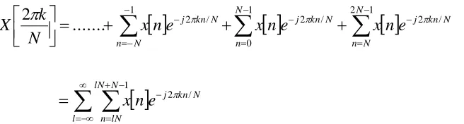
2 _ 2 / _{ }

   



We can divide the summation in (1) into infinite number of summations where each sum

contains N terms.

 

 

 

 

 







If we then change the index in the summation from n to n-l N and interchange the order of

summations we get:

X[w]

w

Dept., of ECE/SJBIT Page 8





2 1

0

/

2  

      _     

 

Denote the quantity inside the bracket as xp[n]. This is the signal that is a repeating version of

x[n] every N samples. Since it is a periodic signal it can be represented by the Fourier series.

 

1

0

/

2  





With FS coefficients:

 

0

/

2  





Comparing the expressions in equations (1.4) and (1.3) we conclude the following:

) 1 ( ,..., 1 , 0 2

1 _{ }

   

 k k N

N X N ck  ………. (1.5)

Therefore it is possible to write the expression xp[n] as below:

 

1

0

/

2  

    



The above formula shows the reconstruction of the periodic signal xp[n] from the samples of

the spectrum X[w]. But it does not say if X[w] or x[n] can be recovered from the samples.

Let us have a look at that:

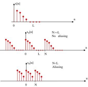
Since xp[n] is the periodic extension of x[n] it is clear that x[n] can be recovered from xp[n] if

there is no aliasing in the time domain. That is if x[n] is time-limited to less than the period N

Dept., of ECE/SJBIT Page 9

Fig. 1.2 Signal Reconstruction

Hence we conclude:

The spectrum of an aperiodic discrete-time signal with finite duration L can be exactly

recovered from its samples at frequencies

N k wk



2

 if N >= L.

We compute xp[n] for n=0, 1,..., N-1 using equation (1.6)

Then X[w] can be computed using equation (1.1).

1.3

Discrete Fourier Transform:

The DTFT representation for a finite duration sequence is ∞ -jωn

X (jω) = ∑ x (n) ℮ n= -∞

jωn

X (n) =1/2π ∫X (jω) e dω , Where ω═ 2πk/n x[n]

n

0 L

xp[n]

n

0 L N

N>=L No aliasing

xp[n]

n

0 N

Dept., of ECE/SJBIT Page 10 2π

Where x(n) is a finite duration sequence, X(jω) is periodic with period 2π.It is

convenient sample X(jω) with a sampling frequency equal an integer multiple of its period =m that is taking N uniformly spaced samples between 0 and 2π.

Let ωk= 2πk/n, 0≤k≤N-1

∞ -j2πkn/N Therefore X(jω) = ∑ x(n) ℮

n=−∞

Since X(jω) is sampled for one period and there are N samples X(jω) can be expressed as

N-1 -j2πkn/N

X(k) = X(jω)│ ω=2πkn/N ═∑ x(n) ℮ 0≤k≤N-1

n=0

1.4

Matrix relation of DFT

The DFT expression can be expressed as

[X] = [x(n)] [WN] T

Where [X] = [X(0), X(1),……..]

[x] is the transpose of the input sequence. WN is a N x N matrix

WN = 1 1 1 1 ………1 1 wn1 wn2 wn3………...wn n-1 1 wn2 wn4 wn6 ………wn2(n-1) ………. ………. 1………..wN (N-1)(N-1)

ex;

4 pt DFT of the sequence 0,1,2,3

X(0) 1 1 1 1 X(1) 1 -j -1 j X(2) = 1 -1 1 -1 X(3) 1 j -1 -j

Solving the matrix X(K) = 6 , -2+2j, -2 , -2-2j

Dept., of ECE/SJBIT Page 11

1.5.1 Relationship of Fourier transform with continuous time signal:

Suppose that xa(t) is a continuous-time periodic signal with fundamental period Tp= 1/F0.The

signal can be expressed in Fourier series as

Where {ck} are the Fourier coefficients. If we sample xa(t) at a uniform rate Fs = N/Tp = 1/T,

we obtain discrete time sequence

Thus {ck’} is the aliasing version of {ck}

1.5.2 Relationship of Fourier transform with z-transform

Let us consider a sequence x(n) having the z-transform

With ROC that includes unit circle. If X(z) is sampled at the N equally spaced points on the

unit circle Zk = e j2πk/N for K= 0,1,2,………..N-1 we obtain

The above expression is identical to Fourier transform X(ω) evaluated at N equally spaced

Dept., of ECE/SJBIT Page 12 If the sequence x(n) has a finite duration of length N or less. The sequence can be recovered

from its N-point DFT. Consequently X(z) can be expressed as a function of DFT as

Dept., of ECE/SJBIT Page 13

Recommended Questions with solutions

Question 1

The first five points of the 8-point DFT of a real valued sequence are {0.25, 0.125-j0.318, 0, 0.125-j0.0518, 0}. Determine the remaining three points

Ans: Since x(n) is real, the real part of the DFT is even, imaginary part odd. Thus the remaining points are {0.125+j0.0518,0,0, 0.125+j0.318}.

Question 2

Compute the eight-point DFT circular convolution for the following sequences. x2(n) = sin 3πn/8

Ans:

Question 3

Dept., of ECE/SJBIT Page 14

Question 4

Define DFT. Establish a relation between the Fourier series coefficients of a continuous time signal and DFT

Solution

The DTFT representation for a finite duration sequence is ∞

X (jω) = ∑ x (n) ℮-jωn

n= -∞

X (n) =1/2π ∫X (jω) e jωn dω , Where ω═ 2πk/n 2π

Where x(n) is a finite duration sequence, X(jω) is periodic with period 2π.It is convenient sample X(jω) with a sampling frequency equal an integer multiple of its period =m that is taking N uniformly spaced samples between 0 and 2π.

Let ωk= 2πk/n, 0≤k≤N

∞ Therefore X(jω) = ∑ x(n) ℮-j2πkn/N

n=−∞

Since X(jω) is sampled for one period and there are N samples X(jω) can be expressed as

N-1

X(k) = X(jω)│ ω=2πkn/N ═∑ x(n) ℮-j2πkn/N 0≤k≤N-1

n=0

Question 5

Solution:-Dept., of ECE/SJBIT Page 15

Question 6

Find the 4-point DFT of sequence x(n) = 6+ sin(2πn/N), n= 0,1,………N-1

Solution :-

Question 7

Dept., of ECE/SJBIT Page 16

Question 8

Solution

Dept., of ECE/SJBIT Page 17

U

NIT

2

P

D

F

T

(DFT)

C

:-

PROPERTIES OF DFT, MULTIPLICATION OF TWO DFTS- THE CIRCULAR CONVOLUTION,

ADDITIONAL DFT PROPERTIES. 6HRS

R

R

1. DIGITAL SIGNAL PROCESSING –PRINCIPLES ALGORITHMS &APPLICATIONS,PROAKIS &

MONALAKIS,PEARSON EDUCATION,4THEDITION,NEW DELHI,2007.

2. DISCRETE TIME SIGNAL PROCESSING,OPPENHEIM &SCHAFFER,PHI,2003.

Dept., of ECE/SJBIT Page 18

Unit 2

Properties of DFT

2.1 Properties:-

In this section we discuss about the important properties of the DFT. These properties are

helpful in the application of the DFT to practical problems.

Periodicity:-

Dept., of ECE/SJBIT Page 19 Then A x1 (n) + b x2 (n)  a X1(k) + b X2(k)

2.1.3 Circular shift:

In linear shift, when a sequence is shifted the sequence gets extended. In circular shift the

number of elements in a sequence remains the same. Given a sequence x (n) the shifted

version x (n-m) indicates a shift of m. With DFTs the sequences are defined for 0 to N-1.

If x (n) = x (0), x (1), x (2), x (3)

X (n-1) = x (3), x (0), x (1).x (2)

X (n-2) = x (2), x (3), x (0), x (1)

2.1.4 Time shift:

If x (n)  X (k)

mk Then x (n-m)  WN X (k)

2.1.5 Frequency shift

If x(n) X(k) +nok

Wn x(n) X(k+no) N-1 kn Consider x(k) = x(n) W n n=0

N-1

(k+ no)n X(k+no)=\ x(n) WN n=0

kn non =  x(n) WN WN

non

 X(k+no)x(n) WN

Dept., of ECE/SJBIT Page 20

X(N-K) = X* (k)

For a complex sequence DFT(x*(n)) = X*(N-K)

If x(n) then X(k)

Real and even  real and even Real and odd  imaginary and odd Odd and imaginary  real odd

Even and imaginary  imaginary and even

2.2 Convolution theorem;

Circular convolution in time domain corresponds to multiplication of the DFTs

If y(n) = x(n)  h(n) then Y(k) = X(k) H(k)

Ex let x(n) = 1,2,2,1 and h(n) = 1,2,2,1 Then y (n) = x(n)  h(n)

Y(n) = 9,10,9,8

N pt DFTs of 2 real sequences can be found using a single DFT

If g(n) & h(n) are two sequences then let x(n) = g(n) +j h(n)

G(k) = ½ (X(k) + X*(k))

H(k) = 1/2j (X(K) +X*(k))

2N pt DFT of a real sequence using a single N pt DFT

Let x(n) be a real sequence of length 2N with y(n) and g(n) denoting its N pt DFT

Let y(n) = x(2n) and g(2n+1) k

X (k) = Y (k) + WN G (k)

Using DFT to find IDFT

Dept., of ECE/SJBIT Page 21 X(n) = 1/N [DFT(X*(k)]*

Recommended Questions with solutions

Question 1

State and Prove the Time shifting Property of DFT

Solution

The DFT and IDFT for an N-point sequence x(n) are given as

Time shift:

If x (n)  X (k)

mk Then x (n-m)  WN X (k)

Question 2

State and Prove the: (i) Circular convolution property of DFT; (ii) DFT of Real and even sequence.

Solution

(i) Convolution theorem

Circular convolution in time domain corresponds to multiplication of the DFTs If y(n) = x(n)  h(n) then Y(k) = X(k) H(k)

Ex let x(n) = 1,2,2,1 and h(n) = 1,2,2,1 Then y (n) = x(n)  h(n)

Y(n) = 9,10,9,8

Dept., of ECE/SJBIT Page 22 If g(n) & h(n) are two sequences then let x(n) = g(n) +j h(n)

G(k) = ½ (X(k) + X*(k)) H(k) = 1/2j (X(K) +X*(k))

2N pt DFT of a real sequence using a single N pt DFT

Let x(n) be a real sequence of length 2N with y(n) and g(n) denoting its N pt DFT Let y(n) = x(2n) and g(2n+1)

X (k) = Y (k) + WNK G (k)

Using DFT to find IDFT

The DFT expression can be used to find IDFT X(n) = 1/N [DFT(X*(k)]*

(ii)DFT of Real and even sequence.

For a real sequence, if x(n) X(k) X (N-K) = X* (k)

For a complex sequence DFT(x*(n)) = X*(N-K)

If x(n) then X(k)

Real and even  real and even Real and odd  imaginary and odd Odd and imaginary  real odd

Even and imaginary  imaginary and even

Question 3

Distinguish between circular and linear convolution

Solution

1) Circular convolution is used for periodic and finite signals while linear convolution is used for aperiodic and infinite signals.

2) In linear convolution we convolved one signal with another signal where as in circular convolution the same convolution is done but in circular pattern depending upon the samples of the signal

3) Shifts are linear in linear in linear convolution, whereas it is circular in circular convolution.

Dept., of ECE/SJBIT Page 23

Solution(a)

Solution(b)

Solution(c)

Dept., of ECE/SJBIT Page 24

Question 5

Solution

Question 6

Dept., of ECE/SJBIT Page 26

U

NIT

3

F

F

T

(FFT)

A

C

:-

USE OF DFT IN LINEAR FILTERING : OVERLAP-SAVE AND OVERLAP-ADD METHOD. DIRECT

COMPUTATION OF DFT, NEED FOR EFFICIENT COMPUTATION OF THE DFT (FFT ALGORITHMS).

7HRS

R

R

1. DIGITAL SIGNAL PROCESSING –PRINCIPLES ALGORITHMS &APPLICATIONS,PROAKIS &

MONALAKIS,PEARSON EDUCATION,4THEDITION,NEW DELHI,2007.

2. DISCRETE TIME SIGNAL PROCESSING,OPPENHEIM &SCHAFFER,PHI,2003.

Dept., of ECE/SJBIT Page 27

UNIT 3

F

AST

-F

OURIER

-T

RANSFORM

(FFT)

ALGORITHMS

3.1 Digital filtering using DFT

In a LTI system the system response is got by convoluting the input with the impulse

response. In the frequency domain their respective spectra are multiplied. These spectra are

continuous and hence cannot be used for computations. The product of 2 DFT s is equivalent

to the circular convolution of the corresponding time domain sequences. Circular convolution

cannot be used to determine the output of a linear filter to a given input sequence. In this case a

frequency domain methodology equivalent to linear convolution is required. Linear

convolution can be implemented using circular convolution by taking the length of the

convolution as N >= n1+n2-1 where n1 and n2 are the lengths of the 2 sequences.

3.1.1 Overlap and add

In order to convolve a short duration sequence with a long duration sequence x(n) ,x(n)

is split into blocks of length N x(n) and h(n) are zero padded to length L+M-1 . circular

convolution is performed to each block then the results are added. These data blocks may be

represented as

The IDFT yields data blocks of length N that are free of aliasing since the size of the

DFTs and IDFT is N = L+M -1 and the sequences are increased to N-points by appending

zeros to each block. Since each block is terminated with M-1 zeros, the last M-1 points from

Dept., of ECE/SJBIT Page 28 block. Hence this method is called the overlap method. This overlapping and adding yields the

output sequences given below.

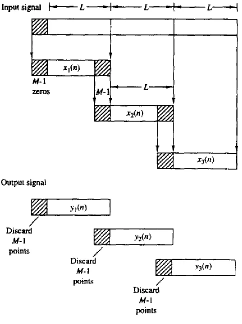
2.1.2 Overlap and save method

In this method x (n) is divided into blocks of length N with an overlap of k-1 samples.

The first block is zero padded with k-1 zeros at the beginning. H (n) is also zero padded to

length N. Circular convolution of each block is performed using the N length DFT .The output

signal is obtained after discarding the first k-1 samples the final result is obtained by adding

Dept., of ECE/SJBIT Page 29 In this method the size of the I/P data blocks is N= L+M-1 and the size of the DFts and

IDFTs are of length N. Each data block consists of the last M-1 data points of the previous

data block followed by L new data points to form a data sequence of length N= L+M-1. An

N-point DFT is computed from each data block. The impulse response of the FIR filter is

increased in length by appending L-1 zeros and an N-point DFT of the sequence is computed

once and stored.

The multiplication of two N-point DFTs {H(k)} and {Xm(k)} for the mth block of data yields

Since the data record is of the length N, the first M-1 points of Ym(n) are corrupted by

aliasing and must be discarded. The last L points of Ym(n) are exactly the same as the result

Dept., of ECE/SJBIT Page 30

3.2 Direct Computation of DFT

The problem:

Given signal samples: x[0], . . . , x[N - 1] (some of which may be zero), develop a procedure to compute

for k = 0, . . . , N - 1 where

We would like the procedure to be fast, simple, and accurate. Fast is the most important, so we will sacrifice simplicity for speed, hopefully with minimal loss of accuracy

3.3 Need for efficient computation of DFT (FFT Algorithms)

Let us start with the simple way. Assume that has been precompiled and stored in a

table for the N of interest. How big should the table be? is periodic in m with period N,

Dept., of ECE/SJBIT Page 31 (Possibly even less since Sin is just Cos shifted by a quarter periods, so we could save just Cos

when N is a multiple of 4.)

Why tabulate? To avoid repeated function calls to Cos and sin when computing the DFT. Now

we can compute each X[k] directly form the formula as follows

For each value of k, there are N complex multiplications, and (N-1) complex additions. There

are N values of k, so the total number of complex operations is

Complex multiplies require 4 real multiplies and 2 real additions, whereas complex additions

require just 2 real additions N2 complex multiplies are the primary concern.

N2 increases rapidly with N, so how can we reduce the amount of computation? By exploiting the following properties of W:

The first and third properties hold for even N, i.e., when 2 is one of the prime factors of N. There are related properties for other prime factors of N.

Divide and conquer approach

We have seen in the preceding sections that the DFT is a very computationally

intensive operation. In 1965, Cooley and Tukey published an algorithm that could be used to

compute the DFT much more efficiently. Various forms of their algorithm, which came to be

known as the Fast Fourier Transform (FFT), had actually been developed much earlier by

other mathematicians (even dating back to Gauss). It was their paper, however, which

stimulated a revolution in the field of signal processing.

Dept., of ECE/SJBIT Page 32 straight forward implementation of the DFT can be computationally expensive because the

number of multiplies grows as the square of the input length (i.e. N2 for an N point DFT). The FFT reduces this computation using two simple but important concepts. The first concept,

known as divide-and-conquer, splits the problem into two smaller problems. The second

concept, known as recursion, applies this divide-and-conquer method repeatedly until the

problem is solved.

Recommended Questions with solutions

Question1

Solution:-Question 2

Dept., of ECE/SJBIT Page 33

Question 3

Dept., of ECE/SJBIT Page 34

Question 4

Solution:- (a)

Dept., of ECE/SJBIT Page 35

U

4

F

F

T

(FFT)

A

C

:-

RADIX-2FFT ALGORITHM FOR THE COMPUTATION OF DFT AND IDFT

DECIMATION IN- TIME AND DECIMATION-IN-FREQUENCY ALGORITHMS. GOERTZEL ALGORITHM, AND CHIRP-Z TRANSFORM. 7HRS

R

R

1. DIGITAL SIGNAL PROCESSING –PRINCIPLES ALGORITHMS &APPLICATIONS,PROAKIS &

MONALAKIS,PEARSON EDUCATION,4THEDITION,NEW DELHI,2007.

2. DISCRETE TIME SIGNAL PROCESSING,OPPENHEIM &SCHAFFER,PHI,2003.

Dept., of ECE/SJBIT Page 36

UNIT 4

R

ADIX

-2

FFT

ALGORITHM FOR THE COMPUTATION OF

DFT

AND

IDFT

4.1 Introduction:

Standard frequency analysis requires transforming time-domain signal to frequency

domain and studying Spectrum of the signal. This is done through DFT computation. N-point

DFT computation results in N frequency components. We know that DFT computation

through FFT requires N/2 log2N complex multiplications and N log2N additions. In certain

applications not all N frequency components need to be computed (an application will be

discussed). If the desired number of values of the DFT is less than 2 log2N than direct

computation of the desired values is more efficient that FFT based computation.

4.2 Radix-2 FFT

Useful when N is a power of 2: N = rv for integers r and v. ‘r’ is called the radix, which comes from the Latin word meaning .a root, and has the same origins as the word radish.

When N is a power of r = 2, this is called radix-2, and the natural .divide and conquer approach. is to split the sequence into two sequences of length N=2. This is a very clever trick

that goes back many years.

4.2.1 Decimation in time

Dept., of ECE/SJBIT Page 38

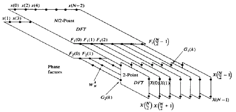
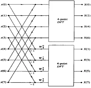
4.2.2 Decimation-in-frequency Domain

Another important radix-2 FFT algorithm, called decimation-in-frequency algorithm is

obtained by using divide-and-conquer approach with the choice of M=2 and L= N/2.This

choice of data implies a column-wise storage of the input data sequence. To derive the

algorithm, we begin by splitting the DFT formula into two summations, one of which involves

the sum over the first N/2 data points and the second sum involves the last N/2 data points.

Thus we obtain

Dept., of ECE/SJBIT Page 39

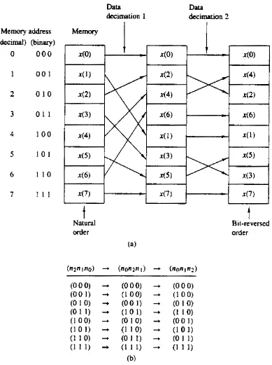
Fig 4.2 Shuffling of Data and Bit reversal

The computation of the sequences g1 (n) and g2 (n) and subsequent use of these

sequences to compute the N/2-point DFTs depicted in fig we observe that the basic

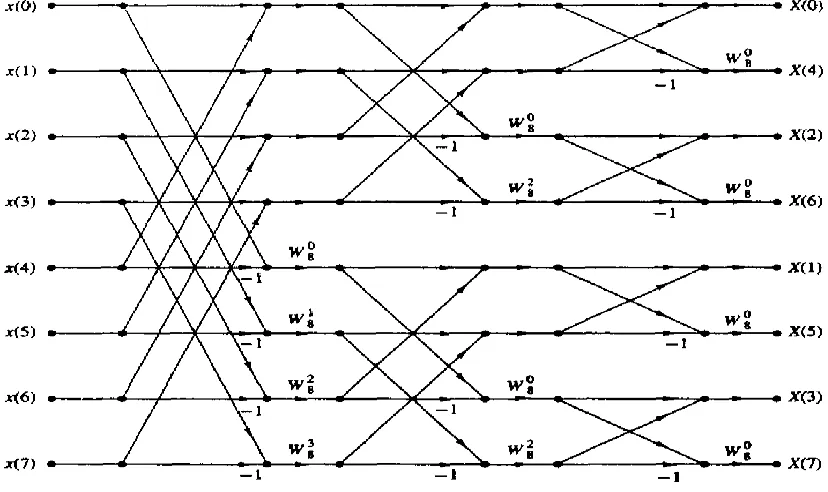
Dept., of ECE/SJBIT Page 40 The computation procedure can be repeated through decimation of the N/2-point DFTs,

X(2k) and X(2k+1). The entire process involves v = log2 N of decimation, where each stage

involves N/2 butterflies of the type shown in figure 4.3.

Dept., of ECE/SJBIT Page 41 Fig 4.4 N=8 point Decimation-in-frequency domain Algorithm

4.2 Example: DTMF – Dual Tone Multi frequency

This is known as touch-tone/speed/electronic dialing, pressing of each button generates a

unique set of two-tone signals, called DTMF signals. These signals are processed at exchange

to identify the number pressed by determining the two associated tone frequencies. Seven

Dept., of ECE/SJBIT Page 42 In this application frequency analysis requires determination of possible seven (eight)

DTMF fundamental tones and their respective second harmonics .For an 8 kHz sampling freq,

the best value of the DFT length N to detect the eight fundamental DTMF tones has been

found to be 205 .Not all 205 freq components are needed here, instead only those

corresponding to key frequencies are required. FFT algorithm is not effective and efficient in

this application. The direct computation of the DFT which is more effective in this application

is formulated as a linear filtering operation on the input data sequence.

This algorithm is known as Goertzel Algorithm

This algorithm exploits periodicity property of the phase factor. Consider the DFT definition

Since is equal to 1, multiplying both sides of the equation by this results in;

This is in the form of a convolution

Where yk(n) is the out put of a filter which has impulse response of hk(n) and input x(n).

The output of the filter at n = N yields the value of the DFT at the freq ωk = 2πk/N

The filter has frequency response given by

The above form of filter response shows it has a pole on the unit circle at the frequency ωk =

2πk/N.

Entire DFT can be computed by passing the block of input data into a parallel bank of N single-pole filters (resonators)

kN N W ) 2 ( ) ( ) ( ) ( 1 0 ) ( 1 0





N x mW x mW

W k X ) ( ) ( )

(n x n h n y_k   _k

) 3 ( ) ( ) ( 1 0 ) (



k n x mW

y ) 4 ( ) ( )

(n W u n h_k  _Nkn

) 6 ( 1 1 )

( _{ 1}

Dept., of ECE/SJBIT Page 43 The above form of filter response shows it has a pole on the unit circle at the frequency ωk =

2πk/N.

Entire DFT can be computed by passing the block of input data into a parallel bank of N single-pole filters (resonators)

1.3 Difference Equation implementation of filter:

From the frequency response of the filter (eq 6) we can write the following difference equation relating input and output;

The desired output is X(k) = yk(n) for k = 0,1,…N-1. The phase factor appearing in the

difference equation can be computed once and stored.

The form shown in eq (7) requires complex multiplications which can be avoided doing suitable modifications (divide and multiply by 1W_Nkz1). Then frequency response of the filter can be alternatively expressed as

This is second –order realization of the filter (observe the denominator now is a second-order expression). The direct form realization of the above is given by

) 7 ( 0 ) 1 ( ) ( ) 1 ( ) ( 1 1 ) ( ) ( ) ( 1            k k k N k k N k k y n x n y W n y z W z X z Y z H ) 8 ( ) / 2 cos( 2 1 1 )

( _{1 2}

Dept., of ECE/SJBIT Page 44 The recursive relation in (9) is iterated for n = 0,1,……N, but the equation in (10) is computed

only once at time n =N. Each iteration requires one real multiplication and two additions.

Thus, for a real input sequence x(n) this algorithm requires (N+1) real multiplications to yield

X(k) and X(N-k) (this is due to symmetry). Going through the Goertzel algorithm it is clear

that this algorithm is useful only when M out of N DFT values need to be computed where M≤

2log2N, Otherwise, the FFT algorithm is more efficient method. The utility of the algorithm

completely depends on the application and number of frequency components we are looking

for.

4.2. Chirp z- Transform

4.2.1 Introduction:

Computation of DFT is equivalent to samples of the z-transform of a finite-length

sequence at equally spaced points around the unit circle. The spacing between the samples is

given by 2π/N. The efficient computation of DFT through FFT requires N to be a highly

composite number which is a constraint. Many a times we may need samples of z-transform

on contours other than unit circle or we my require dense set of frequency samples over a

small region of unit circle. To understand these let us look in to the following situations:

1. Obtain samples of z-transform on a circle of radius ‘a’ which is concentric to unit circle

The possible solution is to multiply the input sequence by a-n

Dept., of ECE/SJBIT Page 45 From the given specifications we see that the spacing between the frequency samples is

π/512 or 2π/1024. In order to achieve this freq resolution we take 1024- point FFT of

the given 128-point seq by appending the sequence with 896 zeros. Since we need

only 128 frequencies out of 1024 there will be big wastage of computations in this

scheme.

For the above two problems Chirp z-transform is the alternative.

Chirp z- transform is defined as:

Where zk is a generalized contour. Zk is the set of points in the z-plane falling on an arc which

begins at some point z0 and spirals either in toward the origin or out away from the origin such

that the points {zk}are defined as,

) 12 ( 1

,.... 1 , 0 )

( 0

0

0

0  

re Re k L

z_k j j k

) 11 ( 1

,... 1 , 0 )

( )

(

1

0

 









L k

z n x z

X

N n

Dept., of ECE/SJBIT Page 46 Note that,

a. if R0< 1 the points fall on a contour that spirals toward the origin

b. If R0 > 1 the contour spirals away from the origin

c. If R0= 1 the contour is a circular arc of radius

d.If r0=1 and R0=1 the contour is an arc of the unit circle.

(Additionally this contour allows one to compute the freq content of the sequence x(n) at

dense set of L frequencies in the range covered by the arc without having to compute a large

DFT (i.e., a DFT of the sequence x(n) padded with many zeros to obtain the desired resolution

in freq.))

e. If r0= R0=1 and θ0=0 Φ0=2π/N and L = N the contour is the entire unit circle similar to the

Dept., of ECE/SJBIT Page 47

Substituting the value of zk in the expression of X(zk)

where

4.2.2 Expressing computation of X(zk) as linear filtering operation:

By substitution of

we can express X(zk) as

Where

both g(n) and h(n) are complex valued sequences

4.2.3 Why it is called Chirp z-transform?

If R0 =1, then sequence h(n) has the form of complex exponential with argument ωn =

n2Φ0/2 = (n Φ0/2) n. The quantity (n Φ0/2) represents the freq of the complex exponential

) 13 ( ) )( ( ) ( ) ( 1 0 0 1 0 0 nk N n n j N n n k

k x n z x n re W

z X       





1 2 2 2

n k k n

nk    

) 16 ( 1 . ,... 1 , 0 ) ( / ) ( ) ( )

(z W 2/2y k  y k h k k L X _k k

2 /

2

) (n Wn

h  0 /2

2 0₎

)( ( )

(n x n rej nW n g    

Dept., of ECE/SJBIT Page 48 signal, which increases linearly with time. Such signals are used in radar systems are called

chirp signals. Hence the name chirp z-transform.

4.2.4 How to Evaluate linear convolution of eq (17)

1. Can be done efficiently with FFT

2. The two sequences involved are g(n) and h(n). g(n) is finite length seq of length N and

h(n) is of infinite duration, but fortunately only a portion of h(n) is required to compute

L values of X(z), hence FFT could be still be used.

3. Since convolution is via FFT, it is circular convolution of the N-point seq g(n) with an

M- point section of h(n) where M > N

4. The concepts used in overlap –save method can be used

5. While circular convolution is used to compute linear convolution of two sequences we

know the initial N-1 points contain aliasing and the remaining points are identical to

the result that would be obtained from a linear convolution of h(n) and g(n), In view of

this the DFT size selected is M = L+N-1 which would yield L valid points and N-1

points corrupted by aliasing. The section of h(n) considered is for –(N-1) ≤ n≤ (L-1)

yielding total length M as defined

Dept., of ECE/SJBIT Page 49 h1(n) = h(n-N+1) n = 0,1,…..M-1

7. Compute H1(k) and G(k) to obtain

Y1(k) = G(K)H1(k)

8. Application of IDFT will give y1(n), for

n =0,1,…M-1. The starting N-1 are discarded and desired values are y1(n) for

N-1 ≤n ≤ M-1 which corresponds to the range 0 ≤n ≤ L-1 i.e.,

y(n)= y1(n+N-1) n=0,1,2,…..L-1

9. Alternatively h2(n) can be defined as

10.Compute Y2(k) = G(K)H2(k), The desired values of y2(n) are in the range

0 ≤n ≤L-1 i.e.,

y(n) = y2(n) n=0,1,….L-1

11.Finally, the complex values X(zk) are computed by dividing y(k) by h(k)

For k =0,1,……L-1

4.3 Computational complexity

In general the computational complexity of CZT is of the order of M log2M complex

multiplications. This should be compared with N.L which is required for direct evaluation.

If L is small direct evaluation is more efficient otherwise if L is large then CZT is more

efficient.

4.3.1 Advantages of CZT

a. Not necessary to have N =L

b.Neither N or L need to be highly composite

c.The samples of Z transform are taken on a more general contour that includes the unit circle as a special case.

4.4 Example to understand utility of CZT algorithm in freq analysis

(ref: DSP by Oppenheim Schaffer)

CZT is used in this application to sharpen the resonances by evaluating the z-transform

off the unit circle. Signal to be analyzed is a synthetic speech signal generated by exciting a 1

)) 1 (

(

1 0

) ( ) ( 2

   

  

   

M n L L

N n h

L n n

Dept., of ECE/SJBIT Page 50 five-pole system with a periodic impulse train. The system was simulated to correspond to a

sampling freq. of 10 kHz. The poles are located at center freqs of 270,2290,3010,3500 & 4500

Hz with bandwidth of 30, 50, 60,87 & 140 Hz respectively.

Solution: Observe the pole-zero plots and corresponding magnitude frequency response for different choices of |w|. The following observations are in order:

• The first two spectra correspond to spiral contours outside the unit circle with a resulting

broadening of the resonance peaks

• |w| = 1 corresponds to evaluating z-transform on the unit circle

• The last two choices correspond to spiral contours which spirals inside the unit circle and

Dept., of ECE/SJBIT Page 51

4.5 Implementation of CZT in hardware to compute the DFT signals

The block schematic of the CZT hardware is shown in down figure. DFT computation

requires r0 =R0 =1, θ0 = 0 Φ0 = 2π/N and L = N.

The cosine and sine sequences in h(n) needed for pre multiplication and post multiplication are

usually stored in a ROM. If only magnitude of DFT is desired, the post multiplications are

unnecessary,

In this case |X(zk)| = |y(k)| k =0,1,….N-1

Dept., of ECE/SJBIT Page 52

Recommended Questions with solutions

Question 1

Solution:-Dept., of ECE/SJBIT Page 53

Question 2

Solution :- There are 20 real , non trial multiplications

Dept., of ECE/SJBIT Page 54

Question 3

Solution:-

Question 4

Dept., of ECE/SJBIT Page 55

Question 5

Solution:-

Question 6

Solution:-

Dept., of ECE/SJBIT Page 57

U

NIT

5

IIR

F

D

C

:-

IIR FILTER DESIGN: CHARACTERISTICS OF COMMONLY USED ANALOG FILTERS –

BUTTERWORTH AND CHEBYSHEVE FILTERS, ANALOG TO ANALOG FREQUENCY

TRANSFORMATIONS. 6HRS

R

R

1. DIGITAL SIGNAL PROCESSING –PRINCIPLES ALGORITHMS &APPLICATIONS,PROAKIS &

MONALAKIS,PEARSON EDUCATION,4THEDITION,NEW DELHI,2007.

2. DISCRETE TIME SIGNAL PROCESSING,OPPENHEIM &SCHAFFER,PHI,2003.

Dept., of ECE/SJBIT Page 58

Unit 5

Design of IIR Filters

5.1 Introduction

A digital filter is a linear shift-invariant discrete-time system that is realized using finite

precision arithmetic. The design of digital filters involves three basic steps:

 The specification of the desired properties of the system.

 The approximation of these specifications using a causal discrete-time system.

 The realization of these specifications using finite precision arithmetic.

These three steps are independent; here we focus our attention on the second step. The

desired digital filter is to be used to filter a digital signal that is derived from an analog signal

by means of periodic sampling. The specifications for both analog and digital filters are often

given in the frequency domain, as for example in the design of low pass, high pass, band pass

and band elimination filters.

Given the sampling rate, it is straight forward to convert from frequency specifications

on an analog filter to frequency specifications on the corresponding digital filter, the analog

frequencies being in terms of Hertz and digital frequencies being in terms of radian frequency

or angle around the unit circle with the point Z=-1 corresponding to half the sampling

frequency. The least confusing point of view toward digital filter design is to consider the filter

as being specified in terms of angle around the unit circle rather than in terms of analog

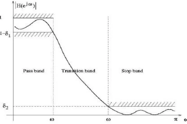
Dept., of ECE/SJBIT Page 59 Figure 5.1: Tolerance limits for approximation of ideal low-pass filter

A separate problem is that of determining an appropriate set of specifications on the

digital filter. In the case of a low pass filter, for example, the specifications often take the form

of a tolerance scheme, as shown in Fig. 5.1.

Many of the filters used in practice are specified by such a tolerance scheme, with no

constraints on the phase response other than those imposed by stability and causality

requirements; i.e., the poles of the system function must lie inside the unit circle. Given a set

of specifications in the form of Fig. 5.1, the next step is to and a discrete time linear system

whose frequency response falls within the prescribed tolerances. At this point the filter design

problem becomes a problem in approximation. In the case of infinite impulse response (IIR)

filters, we must approximate the desired frequency response by a rational function, while in the

finite impulse response (FIR) filters case we are concerned with polynomial approximation.

Dept., of ECE/SJBIT Page 60 The traditional approach to the design of IIR digital filters involves the transformation

of an analog filter into a digital filter meeting prescribed specifications. This is a reasonable

approach because:

 The art of analog filter design is highly advanced and since useful results can be

achieved, it is advantageous to utilize the design procedures already developed for

analog filters.

 Many useful analog design methods have relatively simple closed-form design

formulas.

Therefore, digital filter design methods based on analog design formulas are rather simple to

implement. An analog system can be described by the differential equation

And the corresponding rational function is

The corresponding description for digital filters has the form

and the rational function

In transforming an analog filter to a digital filter we must therefore obtain either H(z)

or h(n) (inverse Z-transform of H(z) i.e., impulse response) from the analog filter design. In

such transformations, we want the imaginary axis of the S-plane to map into the nit circle of

the Z-plane, a stable analog filter should be transformed to a stable digital filter. That is, if the

analog filter has poles only in the left-half of S-plane, then the digital filter must have poles

Dept., of ECE/SJBIT Page 61

5.2 Characteristics of Commonly Used Analog Filters:

From the previous discussion it is clear that, IIT digital filters can be obtained by

beginning with an analog filter. Thus the design of a digital filter is reduced to designing an

appropriate analog filter and then performing the conversion from Ha(s) to H (z). Analog filter

design is a well - developed field, many approximation techniques, viz., Butterworth,

Chebyshev, Elliptic, etc., have been developed for the design of analog low

pass filters. Our discussion is limited to low pass filters, since, frequency transformation can

be applied to transform a designed low pass filter into a desired high pass, band pass and band

stop filters.

5.2.1 Butterworth Filters:

Low pass Butterworth filters are all - pole filters with monotonic frequency response in

both pass band and stop band, characterized by the magnitude - squared frequency response

Where, N is the order of the filter, Ώc is the -3dB frequency, i.e., cutoff frequency, Ώp is the

pass band edge frequency and 1= (1 /1+ε2 ) is the band edge value of │Ha(Ώ)│2. Since the

product Ha(s) Ha(-s) and evaluated at s = jΏ is simply equal to │Ha(Ώ)│2, it follows that

The poles of Ha(s)Ha(-s) occur on a circle of radius Ώc at equally spaced points. From Eq.

(5.29), we find the pole positions as the solution of

Dept., of ECE/SJBIT Page 62 Note that, there are no poles on the imaginary axis of s-plane, and for N odd there will

be a pole on real axis of s-plane, for N even there are no poles even on real axis of s-plane.

Also note that all the poles are having conjugate symmetry. Thus the design methodology to

design a Butterworth low pass filter with δ2 attenuation at a specified frequency Ώs is Find N,

Where by definition, δ2 = 1/√1+δ2. Thus the Butterworth filter is completely

characterized by the parameters N, δ2, ε and the ratio Ώs/Ώp or Ώc.Then, from Eq. (5.31) find

the pole positions Sk; k = 0,1, 2,……..(N-1). Finally the analog filter is given by

5.2.2 Chebyshev Filters:

There are two types of Chebyshev filters. Type I Chebyshev filters are all-pole filters

that exhibit equiripple behavior in the pass band and a monotonic characteristic in the stop

band. On the other hand, type II Chebyshev filters contain both poles and zeros and exhibit a

monotonic behavior in the pass band and an equiripple behavior in the stop band. The zeros of

this class of filters lie on the imaginary axis in the s-plane. The magnitude squared of the

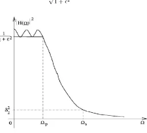
frequency response characteristic of type I Chebyshev filter is given as

Where ε is a parameter of the filter related to the ripple in the pass band as shown in Fig.

(5.7), and TN is the Nth order Chebyshev polynomial defined as

Dept., of ECE/SJBIT Page 63 Where T0(x) = 1 and T1(x) = x.

At the band edge frequency Ώ= Ώp, we have

Figure 5.2: Type I Chebysehev filter characteristic

Or equivalently

Where δ1 is the value of the pass band ripple.

The poles of Type I Chebyshev filter lie on an ellipse in the s-plane with major axis

And minor axis

Dept., of ECE/SJBIT Page 64 The angular positions of the left half s-plane poles are given by

Then the positions of the left half s-plane poles are given by

Where σk =

r

r

Where, by definition δ2 = 1/√1+δ2.

Finally, the Type I Chebyshev filter is given by

A Type II Chebyshev filter contains zero as well as poles. The magnitude squared response is given as

Where TN(x) is the N-order Chebyshev polynomial. The zeros are located on the imaginary

axis at the points

Dept., of ECE/SJBIT Page 65 Where

and

Finally, the Type II Chebyshev filter is given by

The other approximation techniques are elliptic (equiripple in both passband and

stopband) and Bessel (monotonic in both passband and stopband).

5.3 Analog to Analog Frequency Transforms

Frequency transforms are used to transform lowpass prototype filter to other filters like

highpass or bandpass or bandstop filters. One possibility is to perform frequency transform in

the analog domain and then convert the analog filter into a corresponding digital filter by a

mapping of the s-plane into z-plane. An alternative approach is to convert the analog lowpass

filter into a lowpass digital filter and then to transform the lowpass digital filter into the

desired digital filter by a digital transformation.

Suppose we have a lowpass filter with pass edge ΩP and if we want convert that into

another lowpass filter with pass band edge Ω’P then the transformation used is

Dept., of ECE/SJBIT Page 66 Thus we obtain

Dept., of ECE/SJBIT Page 67

Recommended Questions with answers

Question 1

I Design a digital filter to satisfy the following characteristics.

 -3dB cutoff frequency of 0:5_ rad.

 Magnitude down at least 15dB at 0:75_ rad.

 Monotonic stop band and pass band Using

 Impulse invariant technique

 Approximation of derivatives

 Bilinear transformation technique

Figure 5.8: Frequency response plot of the example Solution:-

a) Impulse Invariant Technique

From the given digital domain frequency, _nd the corresponding analog domain frequencies.

Where T is the sampling period and 1/T is the sampling frequency and it always corresponds

to 2Π radians in the digital domain. In this problem, let us assume T = 1sec.

Then Ώc = 0:5Π and Ώs = 0:75Π

Dept., of ECE/SJBIT Page 68 Where δ2 is the gain at the stop band edge frequency ωs.

Order of filter N =5.

Then the 5 poles on the Butterworth circle of radius Ώc = 0:5 Π are given by

Then the filter transfer function in the analog domain is

where Ak's are partial fractions coefficients of Ha(s).

Dept., of ECE/SJBIT Page 69

b)

c) For the bilinear transformation technique, we need to pre-warp the digital frequencies into corresponding analog frequencies.

Then the order of the filter

The pole locations on the Butterworth circle with radius Ώc = 2 are

Then the filter transfer function in the analog domain is

Dept., of ECE/SJBIT Page 70

Question 2

Design a digital filter using impulse invariant technique to satisfy following characteristics

(i) Equiripple in pass band and monotonic in stop band

(ii) -3dB ripple with pass band edge frequency at 0:5П radians.

(iii) Magnitude down at least 15dB at 0:75 П radians.

Dept., of ECE/SJBIT Page 73

Question 3

Solution:-

Dept., of ECE/SJBIT Page 74

Question 4

Dept., of ECE/SJBIT Page 75

U

NIT

6

Implementation of Discrete time systems

C

:-

IMPLEMENTATION OF DISCRETE-TIME SYSTEMS:STRUCTURES FOR IIR AND FIR SYSTEMS DIRECT FORM I AND DIRECT FORM II SYSTEMS, CASCADE, LATTICE AND PARALLEL

REALIZATION. 7HRS

R

R

:-

1. DIGITAL SIGNAL PROCESSING –PRINCIPLES ALGORITHMS &APPLICATIONS,PROAKIS &

MONALAKIS,PEARSON EDUCATION,4THEDITION,NEW DELHI,2007.

2. DISCRETE TIME SIGNAL PROCESSING,OPPENHEIM &SCHAFFER,PHI,2003.

Dept., of ECE/SJBIT Page 76

UNIT 6

Implementation of Discrete-Time Systems

6.1 Introduction

The two important forms of expressing system leading to different realizations of FIR & IIR filters are

a) Difference equation form





 

 

 

 M

k k N

k

ky n k b x n k

a n

y

1 1

) ( )

( )

(

b) Ration of polynomials





  





 _N

k

k k M k

k k

Z a

Z b Z

H

1 0

1 ) (

The following factors influence choice of a specific realization,

 Computational complexity

 Memory requirements

 Finite-word-length

 Pipeline / parallel processing

6.1.1 Computation Complexity

This is do with number of arithmetic operations i.e. multiplication, addition & divisions. If the realization can have less of these then it will be less complex computationally.

In the recent processors the fetch time from memory & number of times a comparison between two numbers is performed per output sample is also considered and found to be important from the point of view of computational complexity.

6.1.2 Memory requirements

This is basically number of memory locations required to store the system parameters, past inputs, past outputs, and any intermediate computed values. Any realization requiring less of these is preferred.

6.1.3 Finite-word-length effects

Dept., of ECE/SJBIT Page 77

6.1.4 Pipeline / Parallel Processing

This is to do with suitability of the structure for pipelining & parallel processing. The parallel processing can be in software or hardware. Longer pipelining make the system more efficient.

6.2 Structure for FIR Systems:

FIR system is described by,



kx n k

b n

y

Or equivalently, the system function



Where we can identify

       otherwise n n b n h n 0 1 0 ) (

Different FIR Structures used in practice are, 1. Direct form

2. Cascade form

3. Frequency-sampling realization 4. Lattice realization

6.2.1 Direct – Form Structure

Convolution formula is used to express FIR system given by,



 It is Non recursive in structure

 As can be seen from the above implementation it requires M-1 memory locations for storing the M-1 previous inputs

 It requires computationally M multiplications and M-1 additions per output point

 It is more popularly referred to as tapped delay line or transversal system

 Efficient structure with linear phase characteristics are possible where )

1 ( )

(n h M n

Dept., of ECE/SJBIT Page 78

Prob:

Realize the following system function using minimum number of multiplication

(1) 1 2 3 4 5

3 1 4 1 4 1 3 1 1 )

(Z   Z  Z  Z  Z Z H We recognize    

 ,1

3 1 , 4 1 , 4 1 , 3 1 , 1 ) (n h

M is even = 6, and we observe h(n) = h(M-1-n) h(n) = h(5-n) i.e h(0) = h(5) h(1) = h(4) h(2) = h(3)

Direct form structure for Linear phase FIR can be realized

Exercise: Realize the following using system function using minimum number of multiplication. 8 7 6 5 3 2 1 4 1 3 1 2 1 2 1 3 1 4 1 1 )

(Z   Z  Z  Z  Z  Z  Z Z H m=9     _{   }

 , 1

4 1 , 3 1 , 2 1 , 2 1 , 3 1 , 4 1 , 1 ) (n h odd symmetry

Dept., of ECE/SJBIT Page 79

6.2.2 Cascade – Form Structure

The system function H(Z) is factored into product of second – order FIR system





 K k

k Z

H Z

H

1

) ( )

(

Where H_k(Z)b_k0b_k1Z1b_k2Z2 k = 1, 2, ….. K and K = integer part of (M+1) / 2

The filter parameter b0 may be equally distributed among the K filter section, such that b0

= b10 b20 …. bk0 or it may be assigned to a single filter section. The zeros of H(z) are grouped

Dept., of ECE/SJBIT Page 80 In case of linear –phase FIR filter, the symmetry in h(n) implies that the zeros of H(z) also exhibit a form of symmetry. If zk and zk* are pair of complex – conjugate zeros then 1/zk and 1/zk* are also a pair complex –conjugate zeros. Thus simplified fourth order sections are formed. This is shown below,

4 3 1 2 2 1 1 0 * 1 1 1 1

0(1 )(1 * )(1 / )(1 / ) ) (                   z z C z C z C C z z z z z z z z C z H k k k k k k k k k k

Problem: Realize the difference equation

) 4 ( ) 3 ( 75 . 0 ) 2 ( 5 . 0 ) 1 ( 25 . 0 ) ( )

(n x n  x n  x n  x n x n y

in cascade form.

Soln: ) ( ) ( ) ( ) 821 . 0 3719 . 1 1 )( 2181 . 1 1219 . 1 1 ( ) ( 75 . 0 5 . 0 25 . 0 1 ) ( ) 75 . 0 5 . 0 25 . 0 1 ){ ( ) ( 2 1 2 1 2 1 4 3 _ 2 1 4 3 2 1 z H z H z H z z z z z H z z z z z H z z z z z X z Y                           

6.3 Frequency sampling realization:

We can express system function H(z) in terms of DFT samples H(k) which is given by

Dept., of ECE/SJBIT Page 81 This form can be realized with cascade of FIR and IIR structures. The term (1-z-N) is realized

as FIR and the term





   

1

0

1 1

) ( 1 N

k

k N z

W k H

N as IIR structure.

The realization of the above freq sampling form shows necessity of complex arithmetic.

Incorporating symmetry in h(n) and symmetry properties of DFT of real sequences the realization can be modified to have only real coefficients.

6.4 Lattice structures

Lattice structures offer many interesting features:

1. Upgrading filter orders is simple. Only additional stages need to be added instead of redesigning the whole filter and recalculating the filter coefficients.

2. These filters are computationally very efficient than other filter structures in a filter bank applications (eg. Wavelet Transform)

3. Lattice filters are less sensitive to finite word length effects.

Consider

i m

i

m i z

a z

X z Y z

H 





 1 ( )

) (

) ( ) (

1

m is the order of the FIR filter and am(0)=1

Dept., of ECE/SJBIT Page 82 y(n)= x(n)+ a1(1)x(n-1)

f1(n) is known as upper channel output and r1(n)as lower channel output.

f0(n)= r0(n)=x(n)

The outputs are

) ( ) ( ), 1 ( 1 ) 1 ( ) ( ) ( 1 ) 1 ( ) ( ) ( 1 1 1 0 0 1 1 0 1 0 1 n y n f then a k if b n r n f k n r a n r k n f n f