Modeling of Deceleration Process of Spatial Movements
Cabir ERGÜVEN
Abstract: Solution of breaking problem of moving mechanical object is
discussed. Five boundary values are used for the problem. Mathematical model of the process has been obtained. Also all dynamic functions and characteristics are represented. They shoe the accuracy of terminal positioning of deceleration.
Keywords: Terminal control, moving objects, boundary problems, adaptive control, reduction, acceleration, transient process, deceleration, positioning of deceleration
Introduction
The spinor model of the kinematics of spatial rotations developed on the basis of spinor representation of generalized spatial rotations [Erguven (2007), Milnikov A.A., Prangishvili A.I., Rodonaia 2005] and the methods of the control theory of terminal states of motion of mechanical objects [Erguven (2007), Batenko A.P. (1977)] made it possible to create simple methods of controlling terminal states of spatial rotations of robot-manipulators. The result has enabled us to reduce the three-dimensional problem of spatial motion control to the one-dimensional problem.
Basics of Model
Let us consider the following technologic task. It is required to bring by means of rotation a mechanical object of control (for instance, a
1 2 3
gripping device or a spherical link) with coordinates x (x , x , x ) to the point
1 2 3
of a three-dimensional space with coordinates y (y , y , y ). An intermediate rotating vector performs rotation by an angle defined by the terminal and initial points of rotation -
) ; ; (ξ1 ξ2 ξ3 ξ
) ) , ( cos( )
* ) , (
cos( 2
x y x ar y x
y x ar
f = =
γ
We have obtained the kinematics expressions for the rotating vectors. [Erguven (2007)]
(1)
where ,
;
.
We have used the rotation angle function s a t i s f y i n g t h e following quite obvious condition:
.
Let us divide the interval into three segments:
, where a , a2 1 < 1 ua = a . 2 1 It is clear that the first segment corresponds to the beginning of the motion process, the second segment to uniform motion and, finally, the third subinterval to deceleration. If we give a = a2 1 , then there will be no uniform motion (the length of the second segment is equal to zero), i.e. the initial stage of motion is immediately followed by the deceleration stage. Later we are discussing only the deceleration stage.
For the deceleration process ending in a complete stop we need to use the problem with five conditions since it is clear that at the end of the rotation process the acceleration must be equal to zero. Therefore the boundary conditions take the following form: [Erguven Cabir, (2006)]
t=0; ; , t=T; ; ; . (2)
Substituting
) ) ( cos ))
( (cos( )
( 2 1 1
1
y x
f t r t r
r x
t γ γ γ
ξ = − −
2
) ) ( cos ))
( (cos( )
( 2 2 2
2
y x
f t r t r
r x
t γ γ γ
ξ = − −
2
) ) ( cos ))
( (cos(
)
( 2 3 3
3
y x
f t r t r
r x
t γ γ γ
ξ = − −
2
) ;
;
(x2y3 x3y2 x3y1 x1y3 x1y2 x2y1
r= − − −
) ;
;
(r2x3 r3x2 r3x1 r1x3 r1x2 r2x1
rx = − − −
) ;
;
(r2y3 r3y2 r3y1 r1y3 r1y2 r2y1
ry = − − −
) (t
γ
) ) , ( cos( )
(
0 2
x y x ar t ≤ f =
≤γ γ
] ; 0
[ γf [0;α1γf]
] ;
[α1γf α2γf [α2γf;γf]
904 . 0
=
into (1) we obtain the following expressions for the rotating vector coordinates as functions of time:
(3)
where K , ω ai (i = 0, 1, 2, 3, 4) and β are defined in [Erguven Cabir, (2006)]. It is not difficult either to calculate the derivatives for (3), but we omit these calculations here because they are too long and tedious.
The values of are equal to the initial deviations from the synthesized control trajectories and define the presence of a transient
∑
= −+
−
−
+
−
=
4 0 0 10 1 10 0 102
)
sin
)
2
)
(
(
cos
)
((
)
(
i i i t Kt
a
t
a
K
a
t
a
e
t
γ
β
γ
γ
β
γ
ω&
ω); ) ) sin ) 2 ) ( ( cos ) (( cos( ) ) sin ) 2 ) ( ( cos ) (( (cos( ) ( 1 4 0 0 10 1 10 0 10 2 1 4 0 0 10 1 10 0 10 2 2 1 y i i i t K x i i i t K f r t a t a K a t a e r t a t a K a t a e r x t
∑
∑
= − = − 2 + − − + + − − + − − + + − − = β γ γ β γ β γ γ β γ γ ξ ω ω ω ω & & ); ) ) sin ) 2 ) ( ( cos ) (( cos( ) ) sin ) 2 ) ( ( cos ) (( (cos( ) ( 2 4 0 0 10 1 10 0 10 2 2 4 0 0 10 1 10 0 10 2 2 2 y i i i t K x i i i t K f r t a t a K a t a e r t a t a K a t a e r x t∑
∑
= − = − 2 + − − + + − − + − − + + − − = β γ γ β γ β γ γ β γ γ ξ ω ω ω ω & & ), ) ) sin ) 2 ) ( ( cos ) (( cos( ) ) sin ) 2 ) ( ( cos ) (( (cos( ) ( 3 4 0 0 10 1 10 0 10 2 3 4 0 0 10 1 10 0 10 2 2 3 y i i i t K x i i i t K f r t a t a K a t a e r t a t a K a t a e r x t∑
∑
= − = − 2 + − − + + − − + − − + + − − = β γ γ β γ β γ γ β γ γ ξ ω ω ω ω & & 0 0 γprocess. When they are equal to the boundary conditions (2) for t = 0, this means that there is no transient process at all. [Erguven Cabir, (2006)]
3. Results of Realization of the Model Deceleration Process
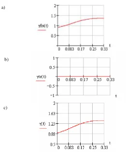
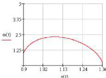
Figures 1? 4 show the dynamic characteristics of the control process on the deceleration segment when
i.e. when there is no transient process – this is clearly seen from Figures. 1.b and 2.b Therefore the curves in Figure. 1.a and Figure. 2.a coincide, since the transient component is absent. Again we see that the control fully satisfies the boundary conditions and in this case the acceleration and the velocity become equal to zero at the end of the given time interval (Figure. 2.c and Figure. 4) , which results in a complete stop.
Figure 1: The deceleration segment (there is no transient process): the rotation angle value as a function of time:
a) the forced component b) the transient component
c) the complete solution: the sum of the forced and transient components
1 905
.
0 10 0
0
10=γ = γ =γ =
γ and & &
b) a)
Figure 2: The deceleration segment (there is no transient process): the rotation angle value as a function of time:
а) the forced component b) the transient component
c) the complete solution: the sum of the forced and transient components
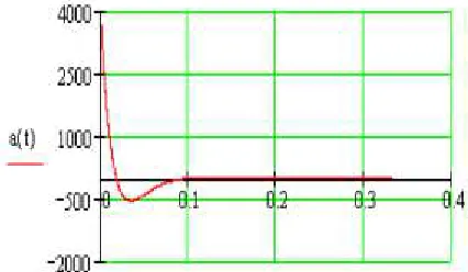
Figure 4: The deceleration segment (there is no transient process): Acceleration as a function time
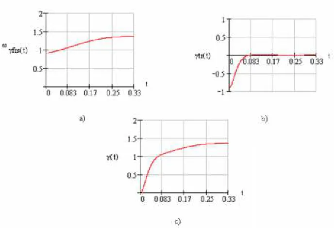
Figure 5: The deceleration segment (there is a transient process): The rotation angle value as a function of time:
a) the forced component b) the transient component
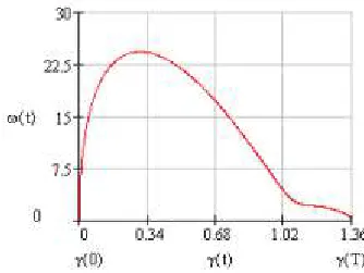
Figure 6: The deceleration segment (there is a transient process): The angular velocity as a function of time
a) the forced component b) the transient component;
c) the sum of the forced and transient components
Figure 8: The deceleration segment (there is a transient process): Acceleration as a function of time
Figures 5? 8 show the dynamic characteristics when
In this case, as seen from Figures. 5.b and 6.b there exists a transient process. As different from the preceding motion stages, in this case the intensity of transient processes is quite comparable with stationary functions though these transient processes damp down soon. It is obvious that the intensity of transient processes explains an essential difference between the stationary and complete functions of angular motion (Figure. 5.a and 5.b) and its velocity (Figure. 6.a and 6.b). Nevertheless the control again satisfies the boundary conditions which gives for the deceleration stage the values
and .
References
1. Erguven Cabir (2007), Analysis and Synthesis of Terminal Control Reduction Problem, Tbilisi, IBSU Journal
2. Erguven Cabir (2007), Control of Terminal Acceleration, Tbilisi, IBSU Journal.
3. Erguven Cabir, (2006), Algorithms of Terminal Control of Spatial Movements of Robots, PhD thesis, Tbilisi, Institute of Mechanics of Machines named after R.Dvali
4. Batenko A.P. (1977) Control of termınal statae of movıng objects, Moscow, Sovetskoe Radıo (Батенко А.П. Управление конечным состоянием движущихся объектов. М.: Советское Радио, 1977, 256 с.
5. Milnikov A.A., Prangishvili A.I., Rodonaia I.D. A Spinor Model of 3-Dimensional Generalized Rotations// // Automation and Remote Control, Moscow, 2005, № 6, p. 30-37
. 0
0 10 0
0
10 =γ = γ =γ =
γ and & &
355 . 1 )
(T1 =γf =