Two-Layer Eddy-Resolving Model of Wind Currents
in the Black Sea
A.A. Pavlushin, N.B. Shapiro, E.N. Mikhailova, G.K. Korotaev
Marine Hydrophysical Institute, Russian Academy of Sciences, Sevastopol, Russian Federation
Processes of formation and variability of the Black Sea circulation are investigated using a two-layer eddy-resolving model. The wind effect only is considered as an exciting force; energy sink takes place due to horizontal turbulent viscosity, friction between the layers and the bottom friction. The rivers’ flowing to the sea and the water exchange through the straits are not taken into account. Numerical approximation requires application of the finite-difference scheme based on the box-method with the grid B (according to the Arakawa terminology), the two-layer scheme of time integrating, the friction implicit approximation nearby the interface and bottom, and the Coriolis force. Being nonlinear, the model, alongside with large-scale circulation, permits to describe vortex structures, formation of which is related to hydrodynamic instability of currents, coastline features, bottom topography and other factors. Discussed are the results of numerical experiments in which, for better understanding of mass transfer and vortex formation processes in the sea, the motion excited by stationary cyclonic winds is considered, whereas bottom topography, friction between the layers, and the β-effect are not taken into account. Relative role of horizontal viscosity and bottom friction is studied. The most interesting results are obtained at mall values of the bottom friction when the motions in the lower layer become significant. It is shown that the model reproduces the major features of the Black Sea circulation, and the most important particular is that it permits to simulate formation and transformation of vortices.
Keywords: the Black Sea, eddy-resolving model, hydrodynamic instability, horizontal and bottom friction.
DOI: 10.22449/1573-160X-2015-5-3-21
© 2015, A.A. Pavlushin, N.B. Shapiro, E.N. Mikhailova, G.K. Korotaev © 2015, Physical Oceanography
Introduction. The purpose of this article is to study the current and vortex formation processes in the Black Sea. To achieve it nonlinear eddy-resolving numerical model (analogous to the one in the Holland – Lin research [1] and covered synoptic vortex modeling in the ocean) is applied.
A great variety of works deal with research and modeling of vortex circulation structure in the Black Sea [2 – 7]. Physical and geographic peculiarities of the synoptic and mesoscale vortices were successfully discovered; possible
mechanisms of their formation were proposed. Eddy-resolving numerical models
are shown to reproduce well the vortex structures having the same parameters as the natural ones. The case in question is mainly about the observations taken from artificial Earth satellites of the sea level (altimetry) and surface temperature.
At the same time, the complexity of the observed pattern, as well as the complexity of the external influence, greatly complicates the interpretation of results obtained. In particular, it is difficult to separate the processes related to the internal dynamics caused by nonlinearity, instability of currents, bottom topography, the configuration of the coasts and the processes directly caused by external influences, in the present case, the wind and its spatial and temporal variability.
Problem statement. We assume wind to be the main factor affecting the seasonal and interannual variability of currents in the Black Sea. Since the Black Sea is significantly baroclinic, the velocity changes occur not only horizontally, but also vertically, which can lead to both barotropic and baroclinic instability of currents.
Liquid with two layers of different density is the simplest model of the baroclinic sea. This model adequately reflects the stratification of the waters of the Black Sea, so it is natural to its use for modeling, as a first approximation, of the dynamic processes in the sea.
Thus, we consider the motion, stimulating by the wind in a two-layer sea. Water density in the upper layer is ρ1=const and in the lower layer –ρ2 =const, whereρ2>ρ1. Surface of the division of the layers z=h(x,y,t)>0 is the surface of the current, i. e. the layers are not mixed with each other; x, y, z – coordinate
axes directed to the east, north and vertically down, respectively; t – time.
Thickness of the upper layerh1=h−ζ , where ζ(x,y,z) is the level, measured down from the undisturbed surface of the sea, thickness of the lower level –
h H
h`2 = − , where H(x,y) is depth of the sea.
Applying the hydrostatic approximations, the Boussinesq ones, β-plane and
assuming that the current velocities do not change with depth within the layer, the equations of motion and continuity can be written as follows:
), ( ) ( ) ( ) ( ) ( ) ( ), ( ) ( ) ( ) ( ) ( ) ( 1 1 1 1 1 2 1 1 1 2 1 1 1 1 1 1 1 1 1 1 1 2 1 1 1 1 1 1 2 1 1 1 h v A gh h u f v v r h v h v u h v h u A gh h v f u u r h u v h u h u l y y y x t l x x y x t ∆ + + = + − + + + ∆ + + = − − + + + τ ζ τ ζ (1) , 0 ) ( ) ( )
(h1 t+ u1h1 x+ v1h1 y = (2)
(3) , 0 ) ( ) ( )
(h2 t + u2h2 x+ v2h2 y = (4)
where (u1,v1),(u2,v2) are horizontal components of the current velocity in the upper and lower layer correspondently; r1,r2 are the friction coefficients in the
division and at the bottom; f = f0+βy is Koriolis parameter,
4 0 10 − = f 1/s, 13 10
2⋅ −
=
β 1/(cm⋅s); g=980cm/s2 is free fall acceleration; g'=g(ρ2−ρ1)/ρ2; y
xτ
τ , are wind tangential stress components; Al is coefficient of horizontal
turbulent viscosity.
Following Holland – Lin [1], we apply the integral equation of continuity ,
0
= + y x V
U (5) that allows to enter an integral function of the current ψ :
, y
U =−ψ V =ψx, (6)
Boundary conditions on the surface of the sea, on surface of the division of the layers and at the bottom are taken into account in deriving the equations (1) – (4). At the side boundaries the adhesion conditions are defined, i.e. equality of the two components of the current velocity:
, 0
= = k k v
u k = 1; 2. (7) River runoff in the sea and water exchange through the straits is not taken into account. Initially, the liquid is in quiescent state, the surface of the division and of the sea are horizontal.
Numerical model. Finite-difference scheme, based on box method with В-grid (according to Arakawa terminology), two-layer time integration scheme, implicit friction approximation on the surface of the division and at the bottom and also the Coriolis force, is used for numerical approximation. Such scheme is usually applied by the authors in the framework of layer quasiisopycnic [8 – 10] and multi-level [11 – 13] models.
Advective terms in the equations of continuity and motion equations are approximated in different ways. In the equations of continuity the approximation by directed differences with the first accuracy order is used; in the equations of motion for the approximation of the advective terms the Lax–Wendroff scheme of the second accuracy order is applied. Accounting of the scheme viscosity in the equations of continuity ensures the stability of the numerical scheme and the positive definiteness of the layer thickness. Application of the Lax–Wendroff scheme to calculate the thickness of the layers leads to the stability of the numerical scheme, with respect to a long term.
In the experiments described, the following sequence of calculations is used.
Let’s assume that the distributions of all fields in the n-moment of time are known.
First, from the equations of continuity there is the thickness of the upper and lower layers: , ] ) ( ) [( 1 n y k k x k k n k n
k u h v h
t h t h + − ∆ = ∆ +
k = 1; 2. (8)
Then the current velocity components and sea level in (n +1)-moment of time
are calculated. Finite-difference analogue of the equations of motion can be written in the following way:
, ) ( ) ( ) ( 1 1 1 1 1 2 1 1 1 1 1 1 1
1 n n
x n n n n L gh u u r h v f t h
u − + − = +
∆ + + + + + ζ , ) ( ) ( ) ( 1 1 1 1 1 2 1 1 1 1 1 1 1
1 n n
y n n n n M gh v v r h u f t h
v + + − = +
∆ + + + + + ζ (9) , ) ( ) ( ) ( 2 1 1 2 1 2 2 1 2 1 1 1 2 2 1 2
2 n n
x n n n n n L gh u r u u r h v f t h
u − − − + = +
∆ + + + + + + ζ , ) ( ) ( ) ( 2 1 1 2 1 2 2 1 2 1 1 1 2 2 1 2
2 n n
y n n n n n M gh v r v v r h u f t h v + = + − − + ∆ + + + + + + ζ
By means of simple calculations the relations between the components of the current velocity and the level slopes can be obtained:
,
* 1 1
1 + +
+ = +Θ −Λ n y k n x k k n
k u
u ζ ζ vkn+1=v*k+Λkζxn+1+Θkζyn+1, (10)
where uk*,v*k are the results of the current velocity calculation at the zero-degree
level slopes and nonzero values of kn
n k M
L , ; functions Θk,Λk are the results of
calculation at the level slopesζx =1, ζy=0 and zero values of n k n k M L , .
Multiplying relations (10) on hkn+1and summing them up under k, we obtain
the expression for the total fluxes:
,
1 1
*
1 + +
+ = + − n
y k n x k k n
k U
U ϑ ζ λζ
(11) ,
1 1
*
1 + +
+ = + + n
y k n x k k n
k V
V λζ ϑ ζ
where Uk,Vk,ϑk,λk
* *
are summed up under k- function of uk,vk,Θk,Λk
* *
.
Solving the relations obtained regarding the level slopes and excluding the level of cross-differentiation after, taking into account the finite-difference
representation of the derivativesζx,ζy, we obtain a system of linear algebraic
equations for the integral function of the current ψn+1in 9-dot pattern. These
equations are solved by over-relaxation with the empirical selection of the optimal relaxation parameter.
Having calculated ψn+1, we find the total flux components, level slopes and
then the velocity components of each layer. Knowing level slopes ζx =A, ζy =B,
we can calculate the level itself, applying the Poisson's equation ∆ζ =Ax+By if
the normal level derivative is known at the border. The Poisson's equation is also solved by means of over-relaxation. Since the level is determined accurate within a constant, and the average level of the area should be equal to zero, then the calculated level should subtract the average value of the area.
Numerical experiments. This formulation of the problem implies that the factors, affecting the circulation formation in the sea, are the spatial and temporal variability of the wind stress, basin shape and coastline features, the intensity of the friction forces, bottom topography, β-effect, and density difference in the upper and lower layers, initial thickness of the upper layer. In the present and the following works we will try to review and analyze the impact of these factors on the results of numerical modeling both individually and in combination with each other.
In a series of experiments, which will be discussed in this article, excluding the
impact of the bottom topography model, β-effect and friction on the surface of the
layer division, the bottom is considered horizontal (H = 2200 m).
For the calculations we applied the rectangular grid with pitches∆x=4 km,
=
The aforementioned free fall acceleration (g'=3.2 cm/s2) and the initial upper
layer thickness (h0 =175 m) were selected in accordance with the observation data
in the Black Sea. In this case the Rossbi deformation radius (Rd = g'h0 f )
equals to 23.4 km and almost six times exceeds the grid pitch, that is necessary for satisfactory description of the vortices[14].
The movement was excited by the stationary cyclonic winds, which is calculated as follows:
, / )
( y
x S x N x S x
l
yτ τ
τ
τ = + − τy=τWy +x(τEy−τWy)/lx, (12)
where τSx,τNx,τWy,τEy are the values τx,τy in accordance with the cardinal points at
the boundaries of the rectangular area [lx×ly], where the Black Sea is inscribed in.
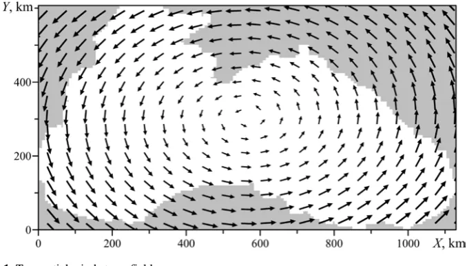
Wind vorticity is constant in such distribution for all points of the basin. In Fig. 1 you can find cyclonic wind field, which was used in this series of experiments and
was obtained by the following formulas (12) when τSx=τEy =0.5cm2/s2,
5 . 0
− = = y
W x N τ
τ cm2/s2.
Calculations were carried out within a 5 – 25 year period, with different values of the coefficients of the horizontal eddy viscosity Aland bottom frictionr2. The
calculations were stopped when the decision came out in a stationary or
quasi-stationary mode. Coefficients Al were selected within the range of sufficiently
small values (102 cm2/s), when nonlinear effects, to relatively large ones
(107 cm2/s) appeared, and when the nonlinearity was negligible. Bottom friction
coefficientsr2 were selected within the range from 0 to 1 cm/s. Coefficient r2, generally speaking, features the adaptation time to the external effects of the
currents in the lower layer 2/ 2,
*
r h
t ≈ i. e.
r
2 = 1 cm/s corresponds to t*≈2 days,where h2 =2 km.
Results of the experiments. The results of the calculations performed were shown on the available potential and kinetic energy diagrams and also spatial
distributions of fieldsh1 and currents in the upper and lower layers u1, u2,
respectively. The most interesting results are available on the website: http://blacksea-model.ru.
Available potential (АPE) and total kinetic (KE) energies were defined the
following way:
, 2 / )
( 1 0 2
1g' h h
АPE= ρ − KE=KE1+KE2,
, 2 / ) ( 12 12
1 1
1 h u v
KE = ρ + KE2= ρ2h2(u22 +v22)/2 ,
where KE1, KE2 is kinetic energy of the upper and lower layer; E=АPE+KE–
total energy; angle brackets mean area averaging.
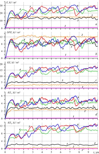
Fig. 2 shows diagrams of the dependence of the energy types from time and
the time at a fixed ratio and sufficiently small bottom friction (r2 =0.01 cm/s) and
various values of horizontal viscosity coefficientAl.
As you can see in the figure, when Al =107 cm2/s the solution has a stationary
form with a close to zero value of the kinetic energyKE2, indicating the substantial
absence of the currents in the lower layer in the stationary case. The energies KE1,
KE, АPE have the lowest values of the given cases.
Under the following decrease of Al to 5⋅10
5
cm2/s energy fluctuations in the
equilibrium mode take a stochastic nature, due to the increasing role of non-linearity of the equations of motion. The kinetic energy of the system increases and
the available potential energy, on the contrary, decreases. The decrease of АPE
has a greater impact on the change in the total energy E, than the increase of KE, as a result the total energy slightly reduces compared with the experiment, where
6
10
=
l
A cm2/s.
Energy diagrams where the values of Al are less than 5⋅10
5
cm2/s, in the
statistically equilibrium mode are characterized by the presence of large amplitude oscillations that occur within certain limits, and also possess stochastic nature. And
the intervals in which the energy changes, are the same for differentAl. As it was
mentioned before, such model behavior at different, relatively small values of
Fig. 2.The time variation of the average area energy components: E(a), APE(b), KE(c), KE1(d), KE2(e) when r2 = 0.01 cm/s and various values Al(1 – Al =107 cm
2
/s; 2 – Al=106 cm2/s; 3 –
5
10 5⋅ =
l
A cm2/s; 4 – =105 l
A cm2/s; 5 – 4
10 =
l
A cm2/s; 6 – 3
10 =
l
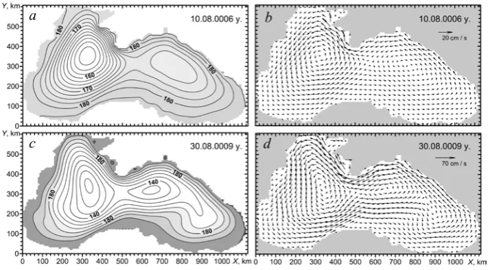
Fig. 3 shows spatial distributions of the upper layer thickness h1 and
currentsu1, obtained during the numerical experiments when entering the statistical
equilibrium mode in the cases Al =107 cm2/с and Al =106 cm2/с.
Fig. 3. Spatial distribution of the upper layer thickness h1, м (a) and velocity of currents u1 (b) where r2=0.01 cm/s, Al =107 cm
2
/s and upper layer thickness h1, м (c), velocity of currents in the upper layer u1 (d) where r2=0.01 cm/s,
6 10
=
l
A cm2/s (areas with greater values of the thickness of the upper layer are marked by darker colour)
Where Al =107 cm
2
/s (Fig. 3, а, b) there is a stationary two-cycled cyclonic rotation in the upper layer. Maximum velocities of the currents up to 20 cm/s are observed near the western border of the Crimean peninsula. But there are
practically no currents in the bottom layer. Field h1 is characterized by two domes
(areas with small layer thickness), which correspond to the centers of cyclonic rotations in the field of currents. From centers of the cycles towards the coast the thickness of the upper layer increases. This situation fully conforms the theory of linear currents in the two-layer liquid, when the circulation is determined by the wind vorticity and configuration of the basin.
Decreasing Al up to 10
6
cm2/s, currents intensify and disturbances in the form of waves appear. They move in the direction of the currents. The pattern of currents remains the same, as there is a cyclonic circulation containing several cores. The maximum velocity of currents in the upper layer reach 60 cm/s, and 10 cm/s – in the lower layer, being also in motion. Fig. 3, c, d shows instantaneous distributions
1
h andu1, where the transformation of fields compared with the previous
experiments can be seen. Click http://blacksea-model.ru/r0.01l6/hb17 and look at this process in motion.
In the further decrease of Al up to 5⋅10
5
in the upper and the lower layers. Formation areas of these vortices are tied to the the coastline features, and the vortices themselves are clearly visible in the velocity field (Fig. 4, c, d). As compared with the previous case (Fig. 3), currents in the upper layer increase slightly, and more significantly – in the lower layer.
Anticyclonic eddies in the field h1 appear in the form of the local maximums of the
layer thickness. It is seen that average year field (Fig. 4, b) is different from the instantaneous field (Fig. 4, a), although it is not quite significant.
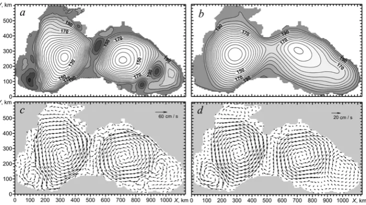
Fig. 4. Spatial distribution of the upper layer thickness h1, m (a), average year thicknessh1, m (b), velocities of currents in the upper layer
1
u (c) and velocities of currents in the lower layer
2 u (d) where r2 = 0.01 cm/s and Al = 5·105 cm2/s for 05.06.0004 (areas with greater values of the thickness of the upper layer are marked by darker colour)
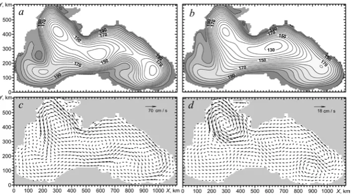
Another interesting situation is observed in the experiments with
5
10
=
l
A cm2/s coefficient (Fig. 5). Two large cyclonic rotations are clearly defined
(«Knippovych glasses»), which periphery quite intense anticyclonic eddies are
formed at. Local maximums h1 refer to the anticyclones. The peculiarities of
circulation are clearly visible both in the topography of the upper layer and the fields of currents in the upper and lower layers. Formation of anticyclonic eddies associated with the hydrodynamic instability has non-stationary nature. They occur sporadically, move in the direction of the current along the coast or move away from the coast with it. In the aforementioned velocity distributions of currents barotropization manifestation of the process can be seen, namely the formation of the unidirectional vortices in same places at the top and bottom layers.
Non-stationary nature of the circulation in the statistical equilibrium mode can
be judged by comparing the instantaneous and average year distributionh1. Thus, in
the average year field h1 the anticyclonic eddies, associated with instability of
Fig. 5. Spatial distribution of the upper layer thickness h1, m (a), average year thicknessh1, m (b), velocities of currents in the upper layer u1 (c) and velocities of currents in the lower layer u2 (d) where r2 = 0.01 cm/s and Al = 5·105 cm2/s for 05.05.0004 (areas with greater values of the thickness of the upper layer are marked by darker colour)
Further, to evaluate the bottom friction impact on the solution of the task the
calculations under Al fixed or different values of r2 ≥0.01 cm/s had been carried
out.
Application of the small values r2 ≤0.001 cm/s in the calculations leads to
appearance of too large velocities of currents in the lower layer, which contradicts
the observations and may cause instability of the pattern during long-term calculations.
The results of the calculations where Al=105 см2/с or r2 are different are
shown in Fig. 6. It can be seen that by increasing the bottom friction
АPEincreases and KEdecreases. The kinetic energy of the upper layer KE1 is
weakly dependent from r2, as opposed to the kinetic energy of the lower layer
2
KE , which sharply decreases with bottom friction coefficient increase. When
0 . 1
2≥
r cm/s, KE2 is practically close to zero. Thus, the total kinetic energy of the
Fig. 6. Time variations of the average area energy components: E(a), APE(b), KE(c), KE1(d), KE2(e) where Al=105 cm2/s and different values r2 (1 – r2=0.01 cm/s; 2 –r2=0.02 cm/s; 3 –
1 . 0
2=
r cm/s; 4 – r2=1.0 cm/s; 5 – r2=10.0 cm/s)
Fig. 7 and 8 show distributions of the upper layer thickness and velocities of currents for the experiments ranging from r2 =0.1 cm/s and r2 =1.0 cm/s.
layer substantially change. Thus, when r2 =0.1 cm/s, the velocities of currents
reach 10 cm/s, and when r2 =1.0cm/s – 2 cm/s. Also, with the increase in the
bottom friction coefficient the intensity of the formation of anti-cyclonic eddies decreases, and they are located to the east of Sinop and to the west of the Crimea.
In the instantaneous and averaged upper layer thickness fields h1 and h1
large-scale cyclonic rotation with two cores is well marked by way of the layer thickness. Increasing the bottom friction, differences between the instantaneous and averaged fields decrease that indicates the more stable circulation.
Spatial distribution of the features when r2>1.0cm/s practically doesn’t differ
from the one shown on the Fig. 8, excluding the velocities in the lower layer which are found close to zero.
Hereby, the performed numerical experiments showed that the examined model permits to obtain the solution within the wide range of horizontal turbulent viscosity coefficients and bottom friction, clearly describes the main features of circulation in the Black Sea, including the formation and transformation of vortices connected with hydrodynamic instability.
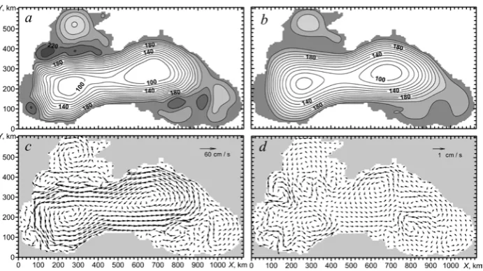
Fig. 7. Spatial distribution of the upper layer thickness h1, m (a), average year thicknessh1, m (b), velocities of currents in the upper layer u1 (c) and velocities of currents in the lower layer u2 (d) wherer2=0.1 cm/s,
5
10
=
l
A см2/с for 10.03.0008 (areas with greater values of the thickness of the upper layer are marked by darker colour)
Fig. 8. Spatial distribution of the upper layer thickness h1, m (a), average year thicknessh1, m (b), velocities of currents in the upper layer u1 (c) and velocities of currents in the lower layer u2 (d) wherer2=1.0 cm/s, Al=105 см2/с for 05.10.0004 (areas with greater values of the thickness of the
upper layer are marked by darker colour)
In the given example, time change of total energy of the system Et is
determined by the joined work W of the tangential wind stressWτ, horizontal
turbulent viscosity coefficients WAL and bottom frictionWR2:
,
2
R AL
t W W W W
E = = τ + + 1( 1 1 ) ,
y x
v u
Wτ = ρ τ + τ
(13) ,
)
( k k k k k k
l k
AL A u u h v v h
W = ρ ∆ + ∆ k=1; 2, ( 22).
2 2 2 2
2 r u v
WR = ρ +
Applying the results of the numerical experiments performed the values of the left and right parts of energy equation were calculated. Fig. 9 shows time diagrams
t
E and W =Wτ +WAL+WR2 where r2=0.01cm/s and various values ofAl. It is obvious that in all the cases there is δ-residual – the difference between calculated
t
E and W. This residual is always negative and connected with the peculiarities of
the numerical scheme applied.
The best results from our viewpoint are obtained when the coefficients Al and
2
r within a relatively narrow range are used: Al is within 10
5
– 1.5⋅105 cm2/с, r2is within 0.005 – 0.01 cm/s. Besides the residual is the least and value closest to WAL
andWR2. When r2 is less than 0.005 cm/s, the velocities in the lower layer
Fig. 9. Diagrams of the time derivative of the total energyEt, joint work W of tangential wind stress forces, horizontal turbulent viscosity, bottom friction and δ-residual when r2=0.01 cm/s and different values of Al (а –Al=103 cm2/s; b –Al=105cm2/s; c – Al=5⋅105 cm2/s; d –
6
10
=
l
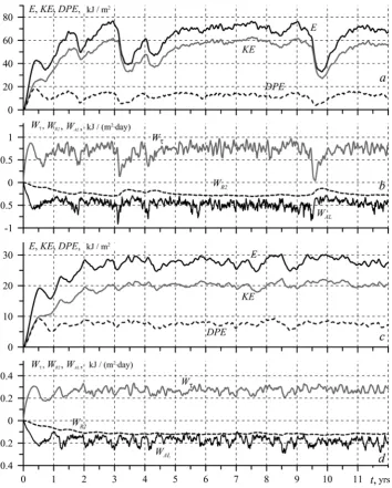
Fig. 10. Time variations of the components of energy E, KE, APE (а, c) work of tangential wind stress forces Wτ, bottom friction WR2, horizontal turbulent viscosity WAL (b, d) where the values of tangential wind stress: а, b – = y=1.0
E x S τ
τ cm2/s2, = y =−1.0
W x N τ
τ cm2/s2; в, г – = y=0.5
E x S τ
τ cm2/s2, 5
. 0 − = = y
W x N τ
τ cm2/s2 (r2=0.007 cm/s,
5
10 4 . 1 ⋅ =
l
A cm2/s)
The fields residualh1,u1,u2 , obtained in the experiments withAl and r2 from
about the currents in the Black Sea [2, 15]. Note that the calculated velocities of currents in the lower layer are higher than actually observed. According to observations in the Black Sea abyssal the velocity of current does not exceed 10 cm/s, and in numerical experiments they can reach 20 – 40 cm/s, of course, in heavy wind and small bottom friction.
The experiments showed that the intensity of the considered cyclonic wind didn’t affect the qualitative circulation pattern in the basin, but only led to the proportional changes of the model energy features. Fig. 10 shows temporary diagrams of energy and work (13) according to the results of two calculations with
different tangential wind stress value (12): where τSx=τEy=1.0cm2/s2,
0 . 1
− = = y
W x N τ
τ cm2/s2и τSx =τEy=0.5 cm2/s2, τNx =τWy =−0.5 cm2/s2.
It is seen that the behavior of the diagrams is the same, except that during the strong wind the values of energy and working force components are greater than when the intensity of the wind is less. The oscillation amplitudes of the features are also greater.
The presence of these oscillations is obviously due to the hydrodynamic instability of currents, which leads to meandering of jet streams and the formation of vortices. This process possesses non-stationary nature and is well marked on the
diagrams of horizontal viscosity and tangential wind stress work forces (Fig. 10, b,
d). These diagrams change in the opposition to the wind work force slight lag.
Process of vortex formation has the least impact on the bottom friction force. It is noteworthy that there are significant changes in the work force of the tangential wind stress during the stationary wind. This is the result of a mismatch of wind fields and currents in the upper layer due to the formation of synoptic and mesoscale eddies opposite to wind vorticity. Thus, as a result of the cross-impact of the wind work force and the vortex formation processes the mechanism of self-oscillation occurs, whereby increasing the energy flow from the wind causes an increase in the vortex formation intensity, resulting in the deformation of current field. Mismatch of wind and current fields leads to a decrease in the energy flow from the wind. Later the synoptic eddies decay by virtue of friction, the field of currents adjusts to the wind, the work force of the wind starts to grow, etc.
Because of the strong non-linearity of the self-oscillation amplitude their period may vary. This variability depends on the strength of the wind. Thus, during
stronger wind (Fig. 10, а, b) as a result of the comparatively small oscillations
sharp falls of the feature values (“gaps”) sporadically occurred.
The fields h1 for several consequent moments of time (Fig. 11) are given for
one of the aforementioned “gaps” taken place in the experiment with the stronger wind. Click http://blacksea-model.ru/experiment_a1.html for details.
There are two domes corresponding to the western and eastern rotations in the
field h1 at the beginning of the examined period (Fig. 11, а). Minimum thickness
1
h in the centers of the cyclones is 90 and 115 m appropriately. The anticyclonic
Fig. 11. Upper layer thicknessh1, м for various moments of time in the experiment with the stationary
wind r2=0.007 cm/s, 5
10 4 . 1 ⋅ =
l
A cm2/s(areas with greater values of the thickness of the layer are marked by darker colour)
In early June a situation happens (Fig. 11, b) when two large-scale cyclones
begin to move toward each other and then get interconnected in the central part of the sea (Fig. 11, c). In the area of Sinop and to the west of the Crimea at this time there are anticyclonic eddies, which are then amplified and moved deeper into the
basin. As shown in Fig. 11, d, e, anticyclonic eddies occupy previous position of
energy diagrams (Fig. 10, a,b) at this time show a sharp fall of the values, which is due to a decrease in the work force of the wind.
The field h1 becomes more even in the next months (Fig. 11, f, g, h),
anticyclonic eddies on the centers of the western and eastern parts of the sea abate, the energy inflow from the wind increases, and gradual restructuring of the field h1 to the form with two large anticyclones on the periphery starts.
Conclusion. The performed experiments showed that the nonlinear two-layer model reproduces the main features of the large-scale circulation of the Black Sea[3, 4, 15], particularly the jet Main Black Sera Current and also the formation and transformation of the vortex structures: large scale cyclonic eddies («Knippovych glasses») and mesoscale eddies caused by meandering of the Main Black Sea Current and hydrodynamic instability processes.
Vortex formations observed in the Black Sea, can be generated by internal nonlinear dynamics even under stationary wind excluding its small-scale features. The self-oscillation mechanism was identified and described. It connects the energy inflow from the wind to the intensity of vortex formation in the sea.
The range of possible values of the horizontal eddy viscosity coefficient and bottom friction, under which the model reproduced the effect of hydrodynamic current instability, had been determined.
The results obtained show two layers to be involved into the vortex formation process. The most intense and relevant observational data vortex formation is obtained when the currents in the lower layer are sufficiently developed. However, this contradicts the observations of the Black Sea currents in the deep-water, which are relatively weak (they do not exceed the speed of 10 cm/s). This may be due to various causes, for example, stationary wind, bottom topography absence or presence of only two layers.
Numerical scheme applied in this model version, has one significant advantage – it allows performing calculations within a wide range of the set parameters and obtaining sustainable solutions. The disadvantage of the scheme is that it does not provide implementation of the energy balance.
The further work is planned to cover the performance of the experiments
devoted to the β-effect study, basin shape, coastline features, bottom topography,
the seasonal variability of the wind, etc., both within the framework of the given model and applying the energy balanced model under the Arakawa scheme.
The objective of the research planned is to analyze the results of the simulation of vortex structures in the oceans obtained by using various numerical schemes. It is expected that it will provide answers to questions about the adequacy reproducible in the numerical experiments, formation circulation mechanisms and temporal evolution of the vortex structures obtained.
Acknowledgements. The works on this subject were carried out under Russian Foundation for Basic Research financial support within the framework of the research project No. 14-45-01044 “r_yug_a." See results of the experiments at http://blacksea-model.ru
REFERENCES
1. Holland, W.R., Lin, L.B., 1975, “On the generation of mesoscale eddies and their contribution to the oceanic general circulation. I. A preliminary numerical experiment. II. A parameter study”, J. Phys. Oceanogr., iss. 5, no. 4, pp. 642-657.
2. Blatov, A.S., Bulgakov, N.P., Ivanov, V.F. [et al.] 1984, “Izmenchivost' gidrofizicheskikh poley Chernogo morya [Variability of hydrophysical fields of the Black Sea]”, Leningrad, Gidrometeoizdat, 239 p. (in Russian).
3. Korotaev, G.K., Saenko, O.A., Koblinsky, C.J. [et al.], 1998, “Tochnost', metodologiya i nekotorye rezul'taty assimilyatsii al'timetricheskikh dannykh TOPEX/POSEIDON v modeli obshchey tsirkulyatsii Chernogo morya [Accuracy, methodology and some assimilation results of TOPEX/POSEIDON altimetric data in the Black Sea general circulation model]”,
Issledovanie Zemli iz kosmosa, no. 3, pp. 3-17.
4. Korotaev, G.K., Saenko, O.A., Koblinsky, C.J., 2001, “Satellite altimetry observation of the Black Sea level”, J. Geophys. Res., iss. 106, no. C1, pp. 911-933.
5. Demyshev, S.G., Knysh, V.V. & Korotaev, G.K., 2003, “Chislennoe modelirovanie sezonnoy izmenchivosti gidrofizicheskikh poley Chernogo moray [Numerical Modeling of the Seasonal Hydrophysical Fields of the Black Sea],” Morskoy gidrofizicheskiy zhurnal, no. 3, pp. 12-27 (in Russian).
6. Demyshev, S.G., 2011, “Chislennyy prognosticheskiy raschet techeniy v Chernom more s vysokim gorizontal'nym razresheniem [Numerical prognostic calculation of the Black Sea currents with high horizontal resolution]”, Morskoy gidrofizicheskiy zhurnal, no. 1, pp. 36-47 (in Russian).
7. Knysh, V.V., Korotaev, G.K. & Moiseenko, V.A. [et al.], 2011, “Sezonnaya i mezhgodovaya izmenchivost' gidrofizicheskikh poley Chernogo morya, vosstanovlennykh na osnove reanaliza za period 1971–1993 gg. [Seasonal and interannual variability of the Black Sea hydrophysical fields reconstructed from 1971-1993 reanalysis data]”, Izv. RAN. Fizika atmosfery i okeana, vol. 47, no. 3, pp. 433-446 (in Russian).
8. Mikhailova, E.N., Shapiro, N.B., 1992, “Kvaziizopiknicheskaya sloistaya model' krupnomasshtabnoy okeanicheskoy tsirkulyatsii [Quasi-isopycnic laminated model of the large-scale ocean circulation]”, Morskoy gidrofizicheskiy zhurnal, no. 4, pp. 3-12 (in Russian) 9. Pavlushin, A.A., Shapiro, N.B., 1996, “Imitatsiya sezonnoy izmenchivosti Atlanticheskogo
okeana v kvaziizopiknicheskoy modeli [Immitation of the Atlantic Ocean seasonal variability within the quasi-isopicnic model]”, Morskoy gidrofizicheskiy zhurnal, no. 4, pp. 12-25 (in Russian).
10. Shapiro, N.B., 1998, “Formirovanie tsirkulyatsii v kvaziizopiknicheskoy modeli Chernogo morya s uchetom stokhastichnosti napryazheniya vetra [Circulation formation within the Black Sea quasi-isopycnic model, including stochastic wind stress]”, Morskoy gidrofizicheskiy zhurnal, no. 6, pp. 26-42 (in Russian).
11. Androsovich, A.I., Mikhailova, E.N. & Shapiro, N.B., 1994, “Chislennaya model' i raschety tsirkulyatsii vod severo-zapadnoy chasti Chernogo morya [Numerical model and calculations of the water circulation in the north-western part of the Black Sea]”, Morskoy gidrofizicheskiy zhurnal, no. 5, pp. 28-42 (in Russian).
12. Mikhailova, E.N., Shapiro, N.B., 2013, “Metod vlozhennykh setok s uluchshennym vertikal'nym razresheniem v pribrezhnoy zone moray [Method of nested grids with a perfected vertical resolution in the coastal zone of the sea]”, Morskoy gidrofizicheskiy zhurnal, no. 4, pp. 3-12 (in Russian).
13. Mikhailova, E.N., Shapiro, N.B. 2014, “Trekhmernaya negidrostaticheskaya model' submarinnoy razgruzki v pribrezhnoy zone moray [Three-dimensional non-hydrostatic model of submarine discharge in the coastal zone]”, Morskoy gidrofizicheskiy zhurnal, no. 4, pp. 28-50 (in Russian).
14. Kamenkovich, V.M., Koshlyakov, M.N. & Monin, A.S., 1982, “Sinopticheskie vikhri v okeane [Synoptic eddies in the ocean]”, Leningrad, Gidrometeoizdat, 264 p. (in Russian) 15. Ivanov, V.A., Belokopytov, V.N., 2011, “Okeanografiya Chernogo morya [Oceanography of