JIEM, 2014 – 7(1): 215-253 – Online ISSN: 2013-0953 – Print ISSN: 2013-8423 http://dx.doi.org/10.3926/jiem.880
Optimization of a Dynamic Supply Portfolio considering
Risks and Discount’s Constraints
Masoud Rabbani, S.M. Khalili, H. Janani, M Shiripour
College of Engineering, University of Tehran (Iran)
[email protected], [email protected], h_jan [email protected], [email protected]
Received: May 2013 Accepted: February 2014
Abstract:
Purpose:
Nowadays finding reliable suppliers in the global supply chains has become so
important for success, because reliable suppliers would lead to a reliable supply and besides that
orders of customer are met effectively. Yet, there is little empirical evidence to support this
view, hence the purpose of this paper is to fill this need by considering risk in order to find the
optimum supply portfolio.
Design/methodology/approach:
This paper proposes a multi objective model for the
Findings:
In order to find a dynamic supply portfolio, we developed a Mixed Integer Linear
Programming (MILP) model which contains two objectives. One objective minimizes the cost
and the other minimizes the risks of delayed, disrupted and defected supplies. CVaR is used as
the risk controlling method which emphases on low-probability, high-consequence events.
Discount option as a common offer from suppliers is also implanted in the proposed model.
Our findings show that the proposed model can help in optimization of a dynamic supplier
selection portfolio with controlling the corresponding risks for large scales of real word
problems.
Practical implications:
To approve the capability of our model various numerical examples
are made and non-dominated solutions are generated. Sensitive analysis is made for
determination of the most important factors. The results shows that how a dynamic supply
portfolio would disperse the allocation of orders among the suppliers combined with the
allocation of orders among the planning periods, in order to hedge against the risks of delayed,
disrupted and defected supplies.
Originality/value:
This paper provides a novel multi objective model for supplier selection
portfolio problem that is capable of controlling delayed, disrupted and defected supplies via
scenario analysis. Also discounts, as an option offered from suppliers, are embedded in the
model. Due to the large size of the real problems in the field of supplier selection portfolio a
meta-heuristic method, NSGA II, is presented for solving the multi objective model. The
chromosome represented for the proposed solving methodology is unique and is another
contribution of this paper which showed to be adaptive with the essence of supplier selection
portfolio problem.
Keywords:
supplier selection, dynamic supply portfolio, conditional value-at-risk, mixed integer
programming, RLTP, NSGA II
1. Introduction and motivation
reasonable to consider the cost lonely, because cost-based approach cannot guarantee quality and on time delivery. In contemporary supply chain management, the performance of potential suppliers is evaluated against multiple criteria rather than considering a single factor-cost. For a suitable choice, many factors are involved such as price, quality, reliability, flexibility, and so on. These factors may contradict each other and may not be satisfied simultaneously (Sawik, 2011a; Ho, Xu & Dey, 2010).
In a risky make-to-order environment, customer-oriented manufacturers should be prepared to produce varieties of products to meet different customer needs. Each product is typically composed of many common and non-common (custom) parts that can be sourced from different approved suppliers with different supply capacities. An important issue is how to allocate the best order of parts among various suppliers so as to fulfill all customer orders of products and to achieve a high customer service level at a low cost and, in addition, to alleviate the impact of supply chain risks. The supply chain risk management has been extensively studied over the past decade (Sawik, 2011b). According to the literature, there are two risk levels: operational risks and disruption risks (Tang, 2006). Operational risks related to the uncertainty such as uncertain customer demand. Disruption risks could be originated from natural disasters (such as earthquakes, etc.) or manmade disasters (such as labor strikes, terrorist attacks, etc.) and caused interruption or failure of the activities. Disruption risks may be seriously detrimental to economy rather than operational risks (Sawik, 2011b). Knemeyer, Zinn and Eroglu (2009) considered a proactive planning for catastrophic events in supply chains, based on an innovative methodology which is used by the insurance industry to quantify the risk of multiple types of catastrophic events on the key supply chain locations.
Despite the stochastic nature of supplier selection problem, a few researches consider uncertainty and risk. Selecting the supply portfolio under variety of risks is a hard discrete stochastic optimization problem. Risk measurement is a key concept in risk management. Two popular methods of risk measurement, which have been used extensively in financial engineering, are value-at-risk (VaR) and conditional value-at-risk (CVaR). VaR estimates maximum loss when cost distribution is symmetric but CVaR determines the maximum loss for undesirable conditions when cost distribution is asymmetric (Sawik, 2011a).
uncertainty in the real-life, fuzzy set theory was used in this model. Also Lee (2009b) suggested FAHP model for supplier selection and applied it for a TFT-LCD manufacturer as a case study. Wu, Zhang, Wu and Olson (2010) presented a fuzzy multi-objective programming for supplier selection with considering quantitative (costs, quality acceptance levels, and on-time delivery distributions) and qualitative (economic, environment and vendor rating) supplier selection risk factors. Xiao, Chen and Li (2012) studied a supplier selection problem under operational risk, for this purpose they extended fuzzy concepts. Sawik (2010) introduced a mixed integer model for supplier selection for make-to-order manufacturing. For controlling risks, the author set an upper limit for average defect rate and late delivery rate. Discount policies are usually considered between buyers and suppliers. Discount offered by the supplier is considered in the model provided by Sawik (2010). Also Sawik (2011c) controlled operational risk by Value-at-Risk (VaR) and Conditional Value-at-Risk (CVaR) for problem of supplier selection in make-to-order environment. Then in (Sawik, 2011b), the portfolio approach was enhanced to consider a single-period supplier selection and supply chain disruption risks. The author controlled this risk by VaR and CVaR concepts. Sawik (2012) considered disruption risks in supplier selection portfolio. He presented models that deal with the optimal selection and protection of part suppliers and order quantity allocation in a supply chain with disruption risks. The objective of model was to achieve a minimum cost of suppliers’ protection, emergency inventory pre-positioning, parts ordering, purchasing, transportation and shortage so as to mitigate the impact of disruption risks by minimizing the potential worst-case cost.
The models were developed for supplier selection and order allocation could be either single-period models that do not consider inventory or multi-single-period models which consider the inventory; however it is obvious that in make-to-order and multi-period environment there is no need to consider inventory. Ustun and Demirtas (2008) studied a objective and multi-period supplier selection problem. For selecting best supplier and optimal allocation, they evaluated all suppliers with fourteen criteria via ANP technique and the multi objective model was solved by multi-objective optimization technique. Sawik (2011a) studied a multi-period supplier selection in the presence of disruption and delay risks. Moreover, the author used VaR and CVaR via scenario analysis.
presented to solve large scales of our model. Also Reservation Level driven Tchebycheff Procedure (RLTP), which is one of the reference point methods, is used to solve small size of our model. To demonstrate the capability of our model numerical examples are generated.
This paper is organized as follows. Related works are presented in the next section. Problem definition and the proposed model are discussed in sections 3 and 4 respectively. Solution methods are suggested in section 6. Numerical examples and some computational results are mentioned in section 7. And finally conclusions and future research directions are made in the last section.
2. Related works
Meena, Sarmah and Sarkar (2011) studied a supplier selection problem under risks of supplier failure due to the catastrophic events disruption. An analytical model is developed to determine the optimal number of suppliers considering different failure probability, capacity, and compensation. Yu, Zeng and Zhao (2009) focused on evaluating the impacts of supply disruption risks on the choice between the famous single and dual sourcing methods in a two-stage supply chain with a non-stationary and price-sensitive demand. Xu and Nozick (2009) formulate a two-stage stochastic program and a solution procedure to optimize supplier selection to hedge against disruptions. Their model allows for the effective quantitative exploration of the trade-off between cost and risks to support improved decision-making in global supply chain design.
Tsai and Wang (2010) applied a mixed integer programming approach to solve the sourcing and order allocation problem with multiple products and multiple suppliers in a supply chain; also two schemes of quantity discounts are used to compare the influence upon the buying decisions. Xia and Wu (2007) developed an integrated approach of analytical hierarchy process improved by rough sets theory and multi-objective mixed integer programming in order to simultaneously determine the number of suppliers to employ and the order quantity allocated to these suppliers in the case of multiple sourcing, multiple products, with multiple criteria and with supplier’s capacity constraints. Authors considered that suppliers may offer price discounts on total business volume, not on the quantity or variety of products purchased from them. Stadtler (2007) presented a linear mixed integer programming (MIP) model, which not only represents the all-units discount but also the incremental discount case.
in the presence of supply disruption. In this regard the author presented a mixed integer programming model in order to find the optimal dynamic supply portfolio. Sawik (2011a) has suggested that the proposed model can be enhanced for a discount environment, where the suppliers offer discounts based on quantity or business volume of ordered parts. Sawik (2010) formulated similar problem of allocating orders for custom parts among suppliers in make to order manufacturing as a mixed integer program model which considers the quantity and business volume discounts offered by suppliers. The proposed model in (Sawik, 2010) considered a single period supplier selection and order allocation problem which provides a static supply portfolio. Sawik (2010) has mentioned to extend the model in a dynamic case where orders arrive irregularly over time.
The proposed model in this paper is a combination of two models which developed by (Sawik, 2010) and (Sawik, 2011a). Indeed, our model is a multi-period supplier selection and order allocation problem which finds the optimal dynamic supply portfolio, and also considers the quantity and business volume discounts offered by suppliers as well. Moreover, time value of money due to interest rate is considered. The developed model and assumptions is described in detail next.
3. Problem description
In this paper, we consider a supply chain in which various types of products are assembled by a single producer and also satisfy customer orders by providing different part types from multiple suppliers. In this supply chain, we will focus on the supplier selection portfolio which is a tactical decision and is made in each period. Due to the multi-period nature of the model, our portfolio will be dynamic. It is not bad to describe a little about the differences between a dynamic and a static supply portfolio. A dynamic supply portfolio is the allocation of orders among the suppliers combined with the allocation of orders among the planning periods, but a static supply portfolio is the allocation of orders for parts among the suppliers without allocation of them among the planning periods (Sawik, 2011a).
using past observations. The supply delays may result in the shortage of required parts and the corresponding delay penalty costs of delayed customer orders will be incorporated into the model.
4. The proposed model
Let I={1,…, M} be the set of M suppliers and J={1,…, N} the set of N part types which are required for the products, this is known ahead of time and not varying over the time horizon. Denote by dj the demand for each part type j є J. The planning horizon consists of H planning periods (e.g. days or weeks) and let T={1,…, H} be the set of planning periods. Assume that supplies are subject to random disruptions. So supplies will be delayed or disrupted (never delivered) in some periods.
The procedure of Sawik (2011a) for calculating delays is as follows. On-time delivery scheduled for period t occurs in that period, whereas the late delivery may occur in one of the remaining periods t+1,…, H, i.e. To deliver the ordered parts by the end of the planning horizon the delay cannot be longer than H-t periods. By convention, deliveries delayed until a dummy period t=H+1 represents disruptions of supplies, i.e. no delivery of ordered parts. Summarizing, it is assumed that the longest delay of each delivery scheduled for period t cannot be greater than H-t periods, whereas the infeasible delay of H-t+1 periods (i.e. delivery in a dummy period t=H+1), by convention represents a disruption, that is, no delivery.
Let us call delivery scenarios by l є L = {1,…, L} so Δl
ijt which is an integer vector, Δlijt є
{0,...,H-t+1}, this represents that delivery of part type j from supplier i є I scheduled for period t є T is either on-time, if Δl
ijt = 0, is delayed by Δlijt periods, if 1 ≤ Δlijt ≤ H-t or is
disrupted, if Δl
ijt = H-t+1. The probability that scenario l for part type j and supplier i occurs in
period t is denoted by Пl
ijt. We assume that the last scenario in the set of scenarios represents
the probability of occurrence the disruption (i.e. scenario L). It is obvious that:
∑
l=1 L
Пijtl =1; i∈I, j∈J, t∈T (1)
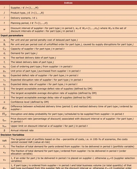
Notations are shown in Table 1.
Now we propose a mixed integer multi objective programming model for selection of a supply portfolio in the presence of supply delays and disruptions with discounts constraints. As mentioned before, the DM needs to select a dynamic supply portfolio, i.e. the allocation of orders for parts among the suppliers and among the planning periods. A dynamic supply portfolio in non-discount environment is defined as:
∑
i∈I
∑
t∈Tand 0 ≤ Fit ≤ 1 is the fraction of the total demand for parts (all parts) ordered from supplier i in period t.
Indices
i Supplier, i є I={1,...,M}
j Product type, j є J={1,...,N}
l Delivery scenario, l є L
t Planning period, t є T={1,...,H}
w Discount interval of supplier i for part type j in period t, wijtє Wijt={1,...,mijt} where Wijt is the set of
discount intervals of supplier i for part type j in period t
Input parameters
aj Per unit and per period penalty cost of delayed part type j
Bj Per unit and per period cost of unfulfilled order for part type j, caused by supply disruptions for part type j
Cijt Capacity of supplier i for part type j in period t
dj Demand for part type j
ej The earliest delivery date of part type j
fj The latest delivery date of part type j
oijt Cost of ordering part type j from supplier i in period t
pijt Unit price of part type j purchased from supplier i in period t
qijt Expected defect rate of supplier i for part type j in period t
rijt Expected disruption rate of supplier i for part type j in period t
sijt Expected delay rate of supplier i for part type j in period t
q The largest acceptable average defect rate of supplies (defined by DM) r The largest acceptable average disruption rate of supplies (defined by DM) s The largest acceptable average delay rate of supplies (defined by DM) α Confidence level (defined by DM)
Δl
ijt Difference between scheduled delivery time (period t) and realized delivery time of part type j ordered by supplier i
Пl
ijt Disruption and delay probability for part type j scheduled to be supplied from supplier i in period t
ξijtw Price discount rate (percentage of discount) associated with discount interval w of supplier i for part type j in period t
bijtw Upper limit on discount interval w of supplier i for part j in period t
β Annual interest rate
Decision Variables
VaR The targeted cost of portfolio based on the cannot exceed VaR (value-at-risk) ∝-percentile of costs, i.e. in 100∝% of scenarios, the costs
Fit The fraction of total demand for parts ordered from supplier i to be delivered in period t (portfolio variable)
xijt The fraction of total demand for part type j ordered from supplier i to be delivered in period t (order allocation variable)
yijt 1, if an order for part j to be delivered in period t is placed on supplier i; otherwise yvariables) ijt=0 (supplier selection
zijt
1, if part type j is ordered from supplier i in period t and total business volume (or total quantity) of that part type purchased from this supplier falls on the discount interval w; otherwise Zijtw=0 (customer order
allocation variable)
Uijtw 1, if total business volume (or total quantity) part type j from supplier i falls on the discount interval w in period t; otherwise = 0
T' Tail cost for delivery scenario l (auxiliary variable to make CVaR equation linear) Qijtw Auxiliary variable for making purchasing cost term in a linear expression
Sawik (2011a) suggested that the dynamic supply portfolio should be checked over the time horizon against the highest acceptable defect rate, delay rate and disruption rate of supplies. Now, denote by q, r and s the maximal acceptable average defect rate, delay rate and disruption rate, respectively. We will trace this suggestion in our model.
In make to order environment, in which custom parts are typically ordered in small lot sizes, supplier may sometimes offer discounts that depends on total value of sales volume (business volume) or on total quantity of ordered parts. In the context of business volume, discount the quantity or variety of purchased parts does not affect the offered price, while for the quantity discount the price does not depend on the total amount of sales volume (Sawik, 2010).
The procedure of Sawik (2010) for considering discount constraints is as follows. Assume that each supplier i offers cumulative (all-units) price breaks having bijtw discount intervals according to the total business volume (or the total quantity), (bijtw-1, bijtw], where bijtw is upper limit on the wth business volume (or quantity) discount interval for supplier i and part j in period t and bijt0=0 for all iєI, jєJ and tєT. Let 0<ξijtw<1 be the discount rate (percentage of discount) associated with interval w of supplier i for part type j in period t. If total business volume (total quantity) from supplier i falls on interval w in period t, then the price of each part type j is ((1-ξijtw).pijt). The following discount interval selection variable needs to be added to enhance the supplier selection and to order allocation problem for the discount environment (Sawik, 2010):
Uijtw=1 if total business volume (or total quantity) for part type j from supplier i falls on the discount interval w in period t; otherwise Uijtw=0.
Furthermore, the order assignment variable Zijwt needs to be clarified as follows:
Zijtw = 1, if parts type j are ordered from supplier i and total business volume (or total quantity) of parts type j purchased from this supplier falls on the discount interval w in period t; otherwise Zijtw = 0.
It is obvious that in make-to-order manufacturing, no inventory of custom parts can be kept on hand and the parts are requisitioned with each customer order. So inventory balance constraints do not need to be considered in the model. In addition, we can assume that parts would be delivered within a time window [ej,fj] and derived from the customer requested due date to reduce any further inventory holding cost. The delivery for part type j cannot be earlier than the earliest date ej. On the other hand, the required parts type j can be delivered late, beyond the latest date fj, or not delivered at all. Then, delay or disruption penalty costs will be charged.
per period cost of unfulfilled order for part type j, caused by supply disruptions for part type j. For delivery scenarios form (l=1) to (l=L-1) and each part type in each period deliveries which are later than fj, are penalized by aj. We can assume that fj is always smaller than H. The total expected delay penalty cost overall delivery scenarios, given an order allocation vector Z, is then given by:
∑
l=1 L
∑
i∈I
∑
j∈Jt∈T: I≤Δlijt∑
≤H−t, fj<t+ΔijtlПijtl a
j(t+Δijtl −fj)djxijt (3)
Note that in equation (3) summations have two following limitations:
Summation on t is only for those parts which their fj are smaller than the sum of the time scheduled for deliveries of them and its corresponding delay of concerned scenario, and
Summation on l is only for scenarios that their corresponding delays are between (1) to (H-t). i.e. those scenarios that show delays not disruptions.
Also it is obvious that if fj=H, then no delivery within the planning horizon can be delayed and penalized. However, any delay beyond H, by convention is a disruption, and hence penalized with the cost of unfulfilled orders (Bj). The total expected penalty cost of unfulfilled orders for parts due to supply disruptions (i.e. deliveries delayed until period H+1) is:
∑
i∈I
∑
j∈Jt∈T : Δ∑
ijtl=H−t+1ПijtL
(Bjdj)xijt (4)
The total business volume or total quantity of parts purchased from supplier i is,
∑
j∈J
∑
t∈Tw∑
∈WijtpijtdjxijtZijtw or
∑
j∈J
∑
t∈Tw∑
∈WijtdjxijtZijtw , respectively. It is clear that these two
expressions are nonlinear and will be made linear by fifth part of constraints in the next section. Notice that the total business volume or the total quantity purchased from each supplier i falls on exactly one discount interval of this supplier, and their phrases are nonlinear that will be reformed to a linear phrase.
Now, the average purchasing and ordering cost for all demand (D) can be expressed as follows:
f(y, Z,x) =
∑
i∈I∑
j∈J∑
t∈Toijtyijt+
∑
i∈I
∑
j∈Jt∑
∈Tw∑
∈Wijt(1−ξijtw)pijtdjZijtwxijt (5)
It is clear that y, Z and x are decision variables. The second part of equation (5) is a nonlinear term so it will be changed to linear term by some constraints and will be mentioned in the next part. Here the performance of the dynamic portfolio with discount in expected costs section can be measured by the sum F(y, Z, x) of average cost per part of ordering, purchasing, defects, delays and disruptions, respectively, in which the cost of a defective parts is assumed to be identical with its regular price:
F(y ,Z, x) = (5) + (
∑
i∈I∑
j∈J∑
t∈TNow the procedure of evaluating the performance of the dynamic supply portfolio in risk section could be clarified. First it is necessary to discuss a little about main general concepts of VaR and CVaR, so for more details interested readers are referred to (Rockafellar & Uryasev, 2002; Uryasev, 2000).
Let αє(0,1) represents the confidence level for the cost distribution across all scenarios. The following two risk measures are commonly used in portfolio selection problems.
VaR at a 100 α% confidence level is the targeted cost of the portfolio such that for 100 α% of the scenarios, the costs will not exceed VaR. In other words, VaR is a parameter (fixed by the DM) or a decision variable based on the α-percentile of costs, i.e. in 100(1-α) % of the scenarios, the costs may exceed VaR. For instance, 90%-VaR is an upper estimation of losses which is exceeded with 10% probability (Rockafellar & Uryasev, 2002; Uryasev, 2000).
CVaR at a 100 α% confidence level is the expected cost of the portfolio in the worst 100(1-α)% of the cases. In other words, we allow 100(1-α) % of the outcomes to exceed VaR, and the mean value of these outcomes is represented by CVaR. So α-conditional Value-at-Risk (α-CVaR) is the minimizing of “the expected value of the costs in the (1-α)100% worst cases” (Rockafellar & Uryasev, 2002; Uryasev, 2000).
VaR represents the maximum cost associated with a specified confidence level of outcomes (i.e. the likelihood that a given portfolio’s cost will not exceed the defined amount of VaR). However, VaR does not explain the magnitude of the cost when the VaR limit is exceeded. In other words, VaR is the acceptable cost level above which we want to minimize the number of realizations and CVaR considers those portfolio outcomes, where costs exceed VaR. CVaR also can be considered as a weighted measure of VaR and the costs above VaR, which may be extremely high costs. When using CVaR to minimize worst-case costs, CVaR is always not less than VaR (Sawik, 2011a).
So we can conclude that the CVaR is a superior than the VaR. Because it is able to quantify losses more efficiently than the discrete distributions, and moreover it is coherent against of the VaR. In addition, optimization of the CVaR leads to optimize of the VaR and also linear programming approaches can be used for minimization of the CVaR. In the dynamic supply portfolio selection problem discussed in this section α is assumed to be fixed by DM to control the risk of losses due to supply delays and disruptions. The DM is willing to accept only portfolios which the total probability of scenarios with costs greater than VaR is not greater than 1-α. Furthermore, the DM wants to minimize the worst-case costs exceeding VaR.
probabilities given as πl for β
l, l=1,…, L (l is representative of an individual scenario) with πl ≥
0 and Ll =
π
1l=
1
å
. For g(x,β), the α-CVaR can be stated by the following minimization formula:Ga(x ,VaR) =VaR+ 1
1−αE[(g(x ,β)−VaR) +
] (7)
Where (g(x,β)-VaR)+ = Max{g(x,β)-VaR,0}.
Let α-CVaR for loss random variable g(x,β) be hα(x). So, the α-CVaR equation can be restated as follows:
hα(x) =min{VaR+ 1
1−αe[Max{g(x,B)−VaR,0}]} (8)
The above model is non-linear programming problem. And so, by considering additional variables Tl for representing Max{g(x,β)-VaR,0} for all (l=1,…, L), this non-linear equation can be transformed into a linear programming model as follows (Uryasev, 2000):
hα(x) =min
{
VaR+ 11−α
∑
l=1 LπlTl
}
(9)S.t.
Tl ≥ g(x,β
l)-VaR; lєL
Tl ≥ 0; lєL
From another point of view Tl can be the amount by which costs (g(x,β
l)) in scenario l exceed
VaR. Thus by the above model the portfolio will be optimized by calculating VaR and minimizing CVaR simultaneously. In our model to select dynamic supply portfolio due to equation (9) for minimizing expected worst-case cost per part we have (corresponding constraints will be mentioned in the next part):
CVaR(x) =VaR+
∑
i∈I∑
j∈J∑
t∈T∑
l∈L Пijtl Tl1−α (10)
Now we summarize equations and phrases in the former section in order to exhibit the complete form of our model.
Objective #1: Minimizing the net present value of expected cost per part (the first objective is like equation (6) with additional coefficients to consider time value of money for each phrase):
F1(y ,Z, x) =
∑
i∈I∑
j∈J∑
t∈Toijtyijt
D(1+β)t+
∑
i∈I∑
j∈Jt∑
∈Tw∑
∈Wijt(1−ξijtw)pijtdjQijtw
D(1+β)t +
∑
i∈I∑
j∈J∑
t∈Tdjpijtqijtxijt D(1+β)t
+
∑
l=1 L−1
∑
i∈I
∑
j∈Jt∈T :1≤Δlijt∑
≤H−t, fj<t+ΔijtlПijtl a j(t+Δijt
l
−fj)djxijt
D(1+β)t +
∑
i∈I∑
j∈Jt∈T : Δ∑
ijtl=H−t+1Пijtl
(Bjdj)xijt
Where:
D=
∑
j=1 N
dj
Objective #2: Selection of dynamic supply portfolio to minimize expected worst-case costs: F2 (Var, T) = Equation (10).
Constraints:
1. Order assignment constraints:
All the demands for each part type in each period are supplied by exactly one supplier in one discount interval.
∑
i∈Iw
∑
∈WijtZijtw=1; j∈J ,t∈T (12)
For each supplier the total quantity of ordered parts cannot exceed its capacity.
djxijt≤cijtyijt; i∈I, j∈J, t∈T (13)
For each part type the total dedications to suppliers must be equal to 1 and corresponding deliveries must not be delivered earlier than the earliest and not later than the latest delivery date.
∑
i∈It∈T : e
∑
j≤t≥fjxijt=1; j∈J (14)
2. Portfolio selection constraints:
The portfolio definition constraint is:
Fit=
∑
j∈J djxijt∑
j∈J
dj ; i∈I, t∈T (15)
The supplier i is selected for delivery of parts in period t if at least one order for part type j is assigned to supplier i in period t.
yijt≥xijt; i∈I, j∈J,t∈T (16)
The average defect rate of the portfolio cannot be greater than q.
∑
i∈I
∑
j∈J∑
t∈Tqijtxijt≤̄q (17)
The average disruption rate of the portfolio cannot be greater than r.
∑
i∈I
∑
j∈J∑
t∈Trijtxijt≤̄r (18)
The average delay rate of the portfolio cannot be greater than s.
∑
i∈I
∑
j∈J∑
t∈TAlso we have the following constraints:
0≤xijt≤1; i∈I, j∈J ,t∈T (20)
0≤fit≤1; i∈I,t∈T (21)
yijt∈{0, 1}; i∈I, j∈J ,t∈T (22)
zijtw∈{0, 1}; i∈I, j∈J,t∈T ,w∈Wijt (23)
3. Risk constraints:
The tail cost of scenario l for all parts which is supplied from all suppliers is defined by the non-negative amount which cost per part in scenario l exceeds VaR,
Tl ≥ Right hand side of equation (11) -VaR; I є L (24)
Tl ≥ 0; I є L (25)
It is worthy to say that the variable VaR does not need to be constrained of being non-negative. Since Tl is constrained of being non-negative, the model tries to decrease VaR and have a positive impact on the objective function. However, large reduction in VaR may result in more scenarios with costs more than VaR (Sawik, 2011a).
Discount constraints are followed by Sawik (Uryasev, 2000) with modifications:
For a business volume discount environment, the total business volume purchased from each selected supplier can be exactly in one discount interval.
(bi, j , t, w−1+1)uijtw≤pijtdjQijtw≤bijtwuijtw; i∈I, j∈J,t∈T ,w∈Wijt (26)
(where Qijtw = xijt zijtw) or
For a quantity discount environment, the total quantity purchased from each selected supplier can be exactly in one discount interval.
(bi, j , t, w−1+1)uijtw≤djQijtw≤bijtwuijtw; i∈I, j∈J,t∈T ,w∈Wijt (27)
(where Qijtw = xijt zijtw)
Parts are ordered from supplier i, if supplier i is selected and assigned at least one part order.
∑
w∈Wijt
uijtw=yijt; i∈I, j∈J, t∈T (28)
zijtw≤uijtw; i∈I, j∈J ,t∈T ,w∈Wijt (29)
Also we have the following constraints.
uijtw∈{0,1}; i∈I, j∈J, t∈T , w∈Wijt (30)
zijtw∈{0, 1}; i∈I, j∈J,t∈T ,w∈Wijt (31)
We define Qijtw = Zijtw. xijt as an auxiliary variable. Then we need to add the following constraints to our model.
Qijtw≥0; i∈I, j∈J,t∈T ,w∈Wijt (32)
Qijtw≤zijtw; i∈I, j∈J, t∈T , w∈Wijt (33)
Qijtw−(M.(1−zijtw)) ≤xijt; i∈I, j∈J, t∈T , w∈Wijt (34)
Qijtw+(M.(1−zijtw)) ≥xijt; i∈I, j∈J, t∈T , w∈Wijt (35)
5. Solution methods
After developing the bi-objective mixed integer program for the dynamic supplier selection portfolio in a discount environment, now we have to propose an appropriate method for solving it. Reviewing literature for the procedure of solving same models shows that most of them solved them in small to medium scales test problems by AMPL programming language and the CPLEX solver (Sawik, 2010; Sawik, 2011c; Sawik, 2011a; Sawik, 2011b; Sawik, 2012). So as our model is multi-objective, we must search methods for solving multi objective models.
For solving small to medium size of our model, we suggest the Reservation Level driven Tchebycheff Procedure (RLTP) that could be coded in common software packages like Lingo or GAMS. This method is announced as a strong method for generating non-dominated solutions by literature for multi objective mathematical models. RLTP is suitable for the proposed model in this paper; because an interactive procedure is made by the DM for determining the tradeoff between worst case costs (CVaR) and expected cost, hence the DM can select the best solution based on his/her risk preference through this method. In fact this approach uses reservation levels based upon DM responses for reducing of the objective space in each of its iterations. Some other advantages of RLTP are that it produces only Pareto-optimal solutions and can solve problems with non-convex nature; also this method is suitable for mixed integer multi-objective models.
objective problems, NSGA-II. This method is so appropriate for solving multi objectives models and has been applied sufficiently in literature of multiple objective models. This method produces Pareto-optimal solutions and is appropriate for mixed integer multi-objective mathematical models.
It should be mentioned that the purpose of this paper is to develop a new model and suggest solution algorithms for the small, medium and large size problems. Undoubtedly other exact and meta-heuristic algorithms may have better results and this requires more discuss that is out of the scope of this paper and could be investigated in the future researches. In what follows, we describe a little about our selected methods i.e. RLTP and NSGA-II. Interested readers can refer to references that will be mentioned.
5.1. The exact solution procedure
The methods of multi-objective optimization have been successfully applied in the literature. Tchebycheff metric based approaches have become popular for sampling the set of nondominated solutions in an interactive search for the most preferred solution in multiple objective decision making situations. These approaches systematically reduce the set of nondominated solutions which remain available for identification and selection from one iteration to the next (Reeves & MacLeod, 1999). Hereafter, we will prepare a little definition about the Reservation Levels Tchebycheff metric Procedure.
Suppose we have K objective functions, in RLTP method first we have to specify the number of solutions to be presented to the DM at each iteration, (P ≥ K), also we need to compute a reference vector, z**, where zi**= max {fi(x) / x є S}+εi and the εi is small positive scalar for each objective. Set Rli=-∞, (i=1,…, K) where RLi is the reservation level for the ith objectives. Second it is necessary to generate a group of 2P dispersed weight vectors, A={λ є Rk / λ
iє(0, 1), ∑λi=1. Third, the associated Tchebycheff program for each weight vector must be solved (the following model):
Min {α-ρ∑zi} (36)
s.t.
α≥ λi(zi**-zi); i=1,…,k fi(x)=zi ; i=1,…,k zi ≥ RLi ; i=1,…,k
xєS
proceed to step 4. Otherwise, have the DM selects his/her current most preferred solution and stop. Forth, DM must partition the current solutions into more and less preferred solution, and adjust the RLs. Now we have to return to step 2 and continuing continue the algorithm. Additional explanation about RLTP can be seen in Reeves & MacLeod (1999).
Using the RLTP algorithm and considering our model constraints, we arrive at a single-objective, mixed integer programming model in each iteration; which can be solved efficiently using a linear programming solver.
5.2. The proposed NSGA-II method
Optimization problems are involved in maximizing or minimizing of the objective value function of the problem in order to satisfy all sets of constraints. If we have only one objective, the problem is considered as single-objective and with the use of the most meta-heuristics algorithms such as tabu search (TS), differential evolution algorithm (DEA), genetic algorithm (GA), simulated annealing (SA), particle swarm optimization (PSO), etc. a near global optimum solution or even global optimum solution can be obtained (Coello, Lamont & Veldhuizen, 2007). But if it is desired to consider more than one objective simultaneously, the problem is considered as multi-objective optimization problem and former algorithms are not proper anymore because they only find one solution in each running, therefore, new algorithms must be designed for these type of problems and the non-dominated sorting genetic algorithm (NSGA) was one of the first proposed algorithms by Srinivas and Deb (1994) for solving multi-objective optimization problems. Highlights of this algorithm are presented as follows:
• Solutions are sorted based on how many solutions are better than the current solution.
• Fitness for solution is assigned based on their rank and non-dominating of other solutions.
• Using fitness sharing method for near solutions in order to solutions’ variations are set properly and solutions are distributed uniformly in search set.
Highlights of this algorithm are presented as follows:
• Using binary tournament selection operator.
• Defining crowding distance as alternative property for fitness sharing.
• Creating and saving non-dominated solutions which are obtained from pervious algorithm steps.
In NSGA-II the same as all evolutionary algorithms (EV), the first step is to create initial population. A good population size is related to the problem, at one side by increasing the population size, the chance of the algorithm to find a better solution will be improved, but at the other side the computational time of the algorithm for searching solutions increases exponentially, in this paper, we consider 100 as the population size. At the second step the fitness functions of all solutions are evaluated which at this paper these values are calculated by equations (10) and (11). If there is only one fitness function we can easily sort solutions but when there is more than one fitness function, the solutions should be ranked and sorted based on all fitness functions, therefore, solutions are divided into two main categories, dominated and non-dominated solutions. In a minimization problem, consider two solutions, m1 and m2, the solution m1 dominates the solution m2 if and only if the following conditions are satisfied.
i є {1, 2,..., n}: fi(m1) ≤ fi(m2) (a)
j є {1, 2,..., n}: fj(m1) ≤ fj(m2) (b)
If both of the above conditions are satisfied, then the solution m1 dominates the solution m2, and m1 is a non-domination solution, but if each one of the conditions (a) or (b) is violated, the solution m1 does not dominate m2, and based on these conditions, the NSGA-II ranks solutions. At the fourth step, some solutions of each generation are selected by the binary tournament selection method. Binary tournament selection method selects randomly two solutions through population, and then compares them and finally the better is selected. Selection criteria in NSGA-II primarily are based on solution rank and after that are based on crowding distance. It is more favorable whatever solution rank is lower and crowding distance is higher.
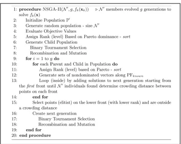
distance. As the same size as main population, members are selected from new population. The selected members create next generation population, and this cycle continues until termination conditions are fulfilled. Figure 1 and Figure 2, show schematic illustration of crowding distance criterion and pseudo-code of the NSGA-II, respectively (more information about these pictures are available in their corresponding references which are noted below them).
Figure 1. Schematic illustration of crowding distance criterion (Boloori Arabani, Zandieh & Ghomi, 2011)
6. Numerical experiments
Now, numerical examples are presented to demonstrate possible applications of the proposed approach for supplier selection portfolio in a discount environment. As we have suggested two solution methods, in this part a test is regarded for each of them. Small size test problems are solved in a reasonable computation time by GAMS. But as the dimension of the test problems grow, computation time is amplified exponentially in GAMS. Hence large size test problems require the meta-heuristic method to be solved.
6.1. Small size test problem with RLTP
6.1.1. Defining parameters
Our small size example includes 3 suppliers; 3 part types; 3 periods; and 3 scenario deliveries. Also we only consider quantity discount constraints in this example with 3 discount intervals for all suppliers and all part types in all periods. For delivery scenarios of supplier i, part type j and period t we assumed that the delivery scheduled for that period occurs either in period t or in period H or not all; i.e. ordered supplies may occur on-time (Δl
ijt= 0; for all i, j, t) or with the
longest delay (Δl
ijt = H-t; for all i, j, t) or never (Δlijt = H-t+1; for all i, j, t). The probabilities of
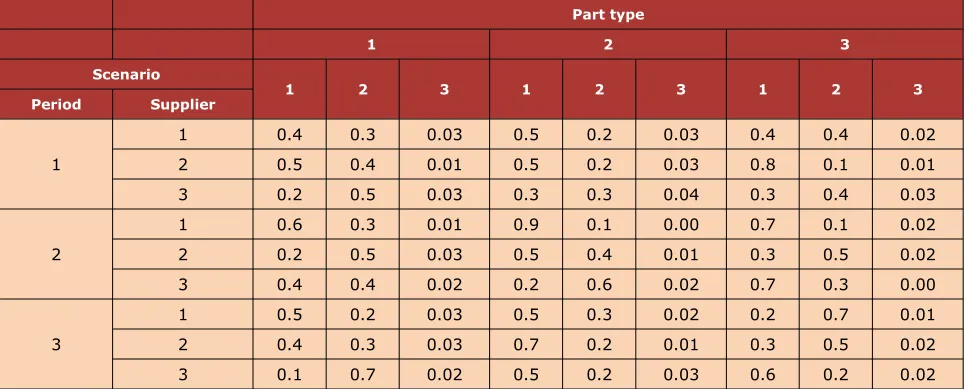
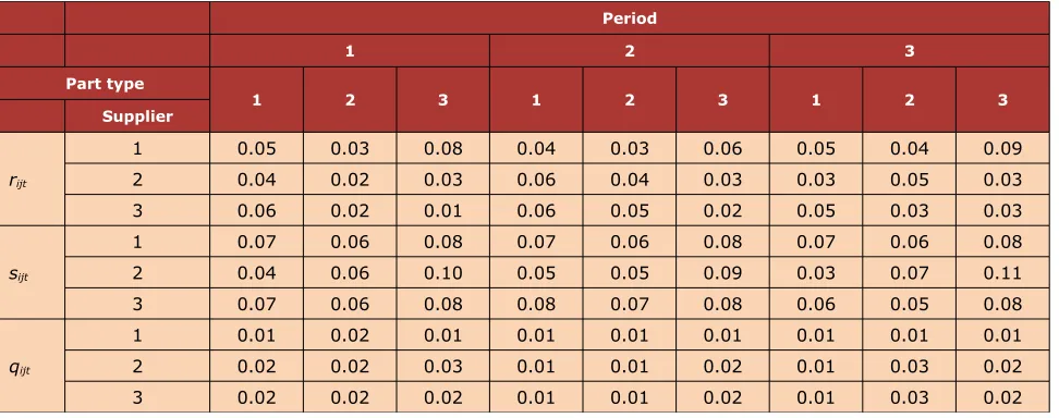
different scenarios (πijtl) are shown in Table 2. It should be noted that we assumed that the probability of occurrence a special scenario in a particular period is independent from earlier periods and their scenarios. Also the source of random generation for other parameters is shown in Table 3, Table 4, Table 5 and Table 6.
Part type
1 2 3
Scenario
1 2 3 1 2 3 1 2 3
Period Supplier
1
1 0.4 0.3 0.03 0.5 0.2 0.03 0.4 0.4 0.02
2 0.5 0.4 0.01 0.5 0.2 0.03 0.8 0.1 0.01
3 0.2 0.5 0.03 0.3 0.3 0.04 0.3 0.4 0.03
2
1 0.6 0.3 0.01 0.9 0.1 0.00 0.7 0.1 0.02
2 0.2 0.5 0.03 0.5 0.4 0.01 0.3 0.5 0.02
3 0.4 0.4 0.02 0.2 0.6 0.02 0.7 0.3 0.00
3
1 0.5 0.2 0.03 0.5 0.3 0.02 0.2 0.7 0.01
2 0.4 0.3 0.03 0.7 0.2 0.01 0.3 0.5 0.02
3 0.1 0.7 0.02 0.5 0.2 0.03 0.6 0.2 0.02
Parameter Value Parameter Value
aj ~Uniform[40;80] (details in Table 4) rijt In Table 6
Bj (details in Table 4) ~Uniform[50;100] sijt In Table 6
Cijt [1.8∑dj /M] for all i and all t q 0.20
dj ~Uniform[120;180]
(details in Table 4) r 0.30
ej 1 for all j s 0.25
fj All parts should be delivered until the end of theperiod that they are ordered in (t) for all j α 0.75
oijt 400 for all i, all j and all t Δlijt Mentioned former
pijt Table 5 Пlijt In Table 2
qijt In Table 6 ξijtw 0.05(w-1) for all i, all j and all t
bijtw [w.cijt/mijt];w=1,…,mijt β 0.20
mijt 3 for all i, all j and all t
Table 3. Values of all parameters
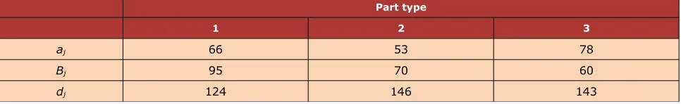
Part type
1 2 3
aj 66 53 78
Bj 95 70 60
dj 124 146 143
Table 4. Values of aj, Bj and dj
Period
1 2 3
Part type
1 2 3 1 2 3 1 2 3
Supplier
pijt
1 20 12 52 20 8 70 21 16 60
2 23 26 60 23 9 72 25 12 54
3 23 12 52 27 12 60 22 13 64
Period
1 2 3
Part type
1 2 3 1 2 3 1 2 3
Supplier
rijt
1 0.05 0.03 0.08 0.04 0.03 0.06 0.05 0.04 0.09
2 0.04 0.02 0.03 0.06 0.04 0.03 0.03 0.05 0.03
3 0.06 0.02 0.01 0.06 0.05 0.02 0.05 0.03 0.03
sijt
1 0.07 0.06 0.08 0.07 0.06 0.08 0.07 0.06 0.08
2 0.04 0.06 0.10 0.05 0.05 0.09 0.03 0.07 0.11
3 0.07 0.06 0.08 0.08 0.07 0.08 0.06 0.05 0.08
qijt
1 0.01 0.02 0.01 0.01 0.01 0.01 0.01 0.01 0.01
2 0.02 0.02 0.03 0.01 0.01 0.02 0.01 0.03 0.02
3 0.02 0.02 0.02 0.01 0.01 0.02 0.01 0.03 0.02
Table 6. Values of expected defect rate, disruption rate and delay rate of supplier i for part type j in period t
6.1.2. Findings through RLTP
The proposed model was solved through coding in GAMS 23.5 and RLTP was implemented for test problems. We developed a mixed integer model (MIP) so the CPLEX solver on a laptop with Intel Core i7 processor running at 2 GHz and with 4GB RAM (DDR3) was used. In what follows, first, we describe the results through the steps of RLTP and after that the final results will be illustrated.
6.1.3. Implementing RLTP for the proposed model
As declared in section 5, to implement RLTP for the mentioned example, following steps are done:
Iteration 1:
As we have 2 (K=2) objectives so we consider presenting 4 (n=4) solutions to the DM at each iteration. Also the best solution for each individual objective is obtained by solving two SOP (Single Objective Programming)model with corresponding constraints, the results are:
Z1*= 23.4764
Z2*= 23.4764
Reservation levels (RLs) for the first iteration will be considered as follows:
RL21= 32 (Second objective reservation level in iteration 1)
Now we generate a group of 8 (=2×n) dispersed weight vectors randomly to use them in the next step. The generated vectors are shown in Table 7:
Objective 1 Objective 2
λ1 0.45 0.55
λ2 0.5 0.5
λ3 0.65 0.45
λ4 0.2 0.8
λ5 0.6 0.4
λ6 0.3 0.7
λ7 0.9 0.1
λ8 0.63 0.37
Table 7. Weight vectors for each objective
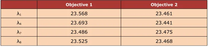
Here we solve the associated AWTP (“Augmented weight Tchebycheff procedure”, for more explanation see Reeves & MacLeod, 1999) model for each λ and present the n (=4) most different (maximally dispersed) of the resulting objective vector to the DM. The results are presented in Table 8.
Objective 1 Objective 2
λ1 23.568 23.461
λ4 23.693 23.441
λ7 23.486 23.475
λ8 23.525 23.468
Table 8. Objective values for selected λ
Now if the DM is satisfied with the best values of each objective, the RLTP will stop; otherwise it is necessary to go the next step that means the next iteration will start. In the proposed example we suppose the DM is not satisfied with the presented values so next iteration will be as follows.
Iteration 2:
The most preferred The least preferred
Objective 1,Objective 2 23.568, 23.461 23.693, 23.441
Objective 1,Objective 2 23.486, 23.475 23.525, 23.468
Table 9. The most and the least preferred of objectives
The RLs have to be adjusted and the following procedure will be used:
For each objective in each iteration, the difference between the worst value of the current most preferred solution for that objective and the worst value for that objective over all current solutions was determined. A percentage of that difference, 50% in this example, was then subtracted from the current most preferred solution value to arrive at the RL for that objective for the next iteration. To illustrate, the worst value of the first objective in the initial most preferred solution was 23.568. The worst initial value for that objective over the set of all current solution was 23.693 for a difference of 0.125. Subtracting 50% of that difference from the worst solution value over the set of all current solution yields a RL for the second iteration of 23.6305. This procedure for the second objective will produce 23.475. Using a higher or lower percentage would decrease or increase the rate of objective space reduction, respectively. The results of this part are:
RL12= 23.6305 (First objective reservation level in iteration 2)
RL22= 23.475 (Second objective reservation level in iteration 2)
After this adjustment, we go back again to step 2 of RLTP.
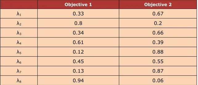
The generated vectors for second iteration are shown in Table 10.
Objective 1 Objective 2
λ1 0.33 0.67
λ2 0.8 0.2
λ3 0.34 0.66
λ4 0.61 0.39
λ5 0.12 0.88
λ6 0.45 0.55
λ7 0.13 0.87
λ8 0.94 0.06
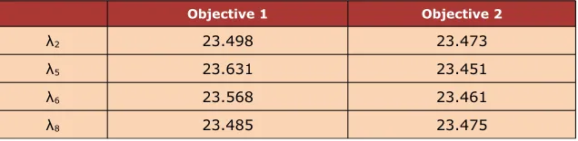
Solving the associated model for each λ and presenting the 4 most different (maximally dispersed) of the resulting objective vector to the DM, is done in Table 11.
Objective 1 Objective 2
λ2 23.498 23.473
λ5 23.631 23.451
λ6 23.568 23.461
λ8 23.485 23.475
Table 11. Objective values for selected λ
Finally in this example we can suppose that the DM is satisfied by solution that is produced by λ6, i.e. 23.568 for objective#1 and 23.461 for objective#2 as the most preferred solution and RLTP is stopped. It is important to emphasis that the RLTP procedure is an interactive way for finding Pareto front. Also RLTP makes it possible to embed the risk preference of the DM by considering different weights for each objective i.e. as the first objective minimizes the expected net present value of costs and the second objective minimizes the worst case costs, so by dedicating larger weights to the first objective we consider the DM as a risk seeker one while by dedicating larger weights for the second objective means considering the DM as a risk avoiding one. Figure 1 shows the Pareto front which was made through two steps of RLTP. In other words the tradeoff between the expected cost and the expected worst-case cost is clearly shown in Figure 1, where the convex efficient frontier of Mean Cost-CVaR model for the confidence level α =0.75 is presented. As mentioned in (Reeves & MacLeod, 1999), RLTP only produces non-dominated solutions and this claim is illustrated in Figure 3.
6.1.4. Presenting and analyzing final results
In this section the details of the selected solution through RLTP (i.e. 23.568 for objective#1 and 23.461 for objective#2) is intended to be described. The model is run and the results are given as follows.
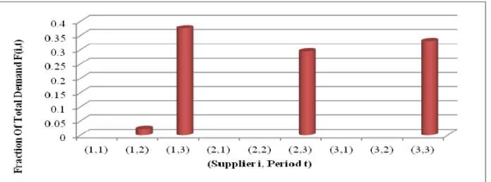
Since the main goal of the model is to determine the portfolio’s variables, we go straight ahead to this part of solution first. The optimal supply portfolios (fraction of total demand dispersed between suppliers in the planning periods) are shown in Figure 6. In Figure 3 average of the defect rate, delay rate disruptions rate for all part types for each period and each supplier are shown. Comparison of Figure 6 and Figure 7 indicate the lowers are defect, disruption and delays rates, the greater is the fraction of total demand. It is also observed that the supplies (i,t) associated with the lowest average disruption and delay rate (1,3) are allotted the largest fraction of total demand. The results indicate that the average disruption and defect rates are key determinants in the decision of dynamic allocation of demand among the suppliers.
Figure 4. Supply portfolio for α=75%
Figure 5. Average of the expected defect rate, expected delay rate and expected disruptions rate for all part types for each period and each supplier
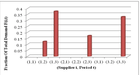
highest 25% of all outcomes scenarios. Now we solve again the example by α=20 %. The resulted portfolio is shown in Figure 8. By comparing Figure 6 and Figure 8 we can see when α increases, a more risk-averse DM increases the number of selected supplies to mitigate the impact of risks by diversification of the supply portfolio (the number of selected supplies is 3 for α=25 % and 4 for α=75 %).
Figure 6. Supply portfolio for α=25%
Figure 7. Supply portfolio for α=75% with an increase in delay and disruption penalizes
Part type 1 2 3
aj 66 53 78
Bj 95 70 60
Table 12. New values of aj, Bj
The computational results for objective values and important variables are summarized in Table 13. As we can see, CVaR measure has a greater or equal value respect to VaR measure. The results acquired for risk measures in Table 13 confirm this judgment. The result of the VaR for α=0.75 in test problem shows that the smallest value such that probability that loss exceeds or equals to this value (23.461) is not larger than 1-α (25%). Because of discrete distribution of scenarios and little number of scenarios, in high confidence level the VaR and CVaR values lead to equal values; however, in less confidence level the difference of these two risk measures is appeared (for α=0.25). Also, obviously, by increasing in confidence level the VaR and CVaR measures increase respect to measures with less confidence level. The results in Table 13 confirm this idea. It can be concluded the CVaR measure is more conservative than VaR measure and so, it is more suitable for risk-averse DMs. In Table 14 the size of mixed integer program is represented by the total number of variables, number of binary variables, number of constraints, and number of non-zero coefficients in the constraint matrix.
Values
Confidence level α=0.75 α=0.25
RLTP Objective 0.002 0.0003
Objective#1 (Expected cost) 23.568 23.476
Objective#2 (CVaR) 23.461 23.374
VaR 23.461 22.777
Portfolio variable (Fit)
F12=0.022
F13=0.375
F23=0.273
F33=0.330
F13=0.375
F23=0.295
F33=0.330
Order allocation variable (xijt)
X122=0.074
X133=1
X223=0.926
X313=1
X133=1
X223=1
X313=1
Table 13. The solution results for multi objective model by the selected solution by weight vector λ6 in Table 10
Total number of variables Number of binary variables Number of equations Number of non-zero coefficients
314 189 475 1799
6.2. Large size test problem with NSGA-II
In this part we develop a test problem for large size problems that includes 5 suppliers; 10 part types; 12 periods; 3 delivery scenarios and 5 discount intervals. This size of model can be considered as a real size that can be applicable in real word. To demonstrate the capability of our meta-heuristic algorithm first we tried to make some non-dominated solutions by RLTP and then by our NSGA-II method for this test problem. Hence, we can compare solutions and see how good NSGA-II method is. It should be noted that a lot of test problems were made by the provided code in MATLAB (R 2010a version) (MATLAB, 2010), but for a lot of test problems RLTP method which is coded by GAMS could not make any solutions after a long time, so the comparison with our NSGA-II was not possible. Parameters of the proposed model are shown in Table 15.
Parameter Value Parameter Value
aj ~ Uniform [100; 200] rijt ~Uniform [0.001;0.009]
Bj ~ Uniform [200;400] sijt ~Uniform [0.001;0.004]
Cijt ~ Uniform [500;700] q 0.95
dj ~ Uniform [300; 700] r 0.80
ej 1 for all j s 0.97
fj All parts should be delivered until the end ofthe period they are ordered in (t) for all j α 0.75
oijt ~ Uniform [100;150] Δlijt Mentioned former
pijt ~ Uniform [500;700] Пlijt ~Uniform [0.05;0.25](for l=1,…,l=L-1)
qijt ~ Uniform [0.001;0.004] Пlijt ~Uniform [0.01;0.12](for l=L)
bijtw [w.cijt/mijt]; w= 1,…,(mijt=40) ξijtw 0.05(w-1) for all i, all j and all t
mijt 40 for all i, all j and all t β 0.20
Table 15. Values of all parameters
As mentioned in section 5, RLTP method needs the best possible solution of each objective individually. CPLEX solver after a considerable time and gap made the following results for each objective.
Z1* = 92.184508 (Absolute gap: 54.232942)
Z2* = 97.654553 (Absolute gap: 68.425849)
Reservation levels (RLs) for the first iteration will be considered as follows:
RL11 = 200 (First objective reservation level in iteration 1)
As we have 2 (K=2) objectives so we will consider to present 8 (n=8) solutions to the DM at each iteration. So we randomly generate a group of 16 (=2×n) dispersed weight vectors to use them in the next step. The generated vectors are shown in Table 16.
Objective 1 Objective 2
λ1 0.4 0.6
λ2 0.6 0.4
λ3 0. 5 0.5
λ4 0.3 0.7
λ5 0.7 0.3
λ6 0.55 0.45
λ7 0.18 0.82
λ8 0.38 0.62
λ9 0.43 0.57
λ10 0.21 0.79
λ11 0.38 0.62
λ12 0.71 0.29
λ13 0.78 0.22
λ14 0.69 0.31
λ15 0.03 0.97
λ16 0.59 0.41
Table 16. Weight vectors for each objective
Here we solve the associated AWTP (“Augmented weight Tchebycheff procedure”, for more information see Reeves & MacLeod (1999)) model for each λ and present the n (=3) most different (maximally dispersed) of the resulting objective vector to the DM. The results, which are presented in Table 16 and RLTP, are stopped after one iteration. It should be noted that the solutions for each λ had considerable gap for RLTP objective function that those gaps are shown in the last column of Table 17.
Objective 1 Objective 2 RLTP objective functionabsolute gap
λ2 99.023 123.286 1.05819
λ4 103.163 122.458 1.050982
λ6 101.066 123.322 1.060341
λ7 103.286 120.944 1.046173
λ9 100.158 127.046 1.072544
λ13 98.720 122.201 1.177907
λ14 102.107 122.045 1.121844
λ16 104.298 123.850 1.083998
NSGA-II method made the following results for each objective. Results of iterations 57, 100 and 350 are illustrated in Table 18.
Iteration Objective 1 Objective 2
57
98.9398692 212.2468078 104.4850313 97.65857192 100.4196316 116.9182974 101.8503318 102.0474934 103.050333 97.81699661 102.3275586 99.30488047 102.869205 98.0832395
100
98.9398692 212.2468078 104.0845977 97.30380731 99.5061131 115.2043315 99.5061131 115.2043315 99.94955866 101.7087943
350
95.89775 99.28186964 100.2331273 94.4763972 97.96652779 94.79240783 100.0887156 94.58571687
Table 18. Objective values for selected λ
Now in Figure 8, we can comprise RLTP and NSGA-II methods. As shown in this figure NSGA-II has made more dispersed and a lot better solutions than NSGA-II. Also RLTP has a lot of difficulty in finding the best solution of each objective individually as well as in finding the solution of RLTP objective function. Details of one solution through RLTP for instance are shown in Table 19 and Table 20; also Figure 9, depicts the results of portfolio variables which are the most important results of the model. The same sensitive analysis like section 6.1.4 can be developed for large scales, but for avoidance of repetition they are not motioned again here.
Iteration 350
Objective#1 100.0887
Objective#2 (CVaR) 94.58572
Confidence Level 0.75
Table 19. Objective’s values and confidence level of NSGA-II for the proposed test problem
Supplier
1 2 3 4 5
Period
1 0.000435 0.005685 0.003427 0.002858 0.001869
2 0 0.003182 0.001667 0.003968 0.005457
3 0 0.003181 0.001869 0 0.009224
4 0 0.007535 0.004192 0.000678 0.001869
5 0.008436 0 0.001869 0.003181 0.000787
6 0.0029 0.001667 0.003695 0.003181 0.002831
7 0.002304 0.004848 0.003588 0 0.003534
8 0 0.004373 0.006717 0.000435 0.002749
9 0.005515 0.000678 0.005577 0.002504 0
10 0.005635 0.001741 0.001869 0.005029 0
11 0.087507 0.088612 0.002504 0.002254 0
12 0 0.1686 0.335864 0 0.171919
Table 20. Results of portfolio variables (Fit) resulted from NSGA-II
Figure 9. Values of supply portfolio variables for α=75% in a large size test problem
7. Conclusion and future research
be applied for the selection of suppliers and the allocation of orders quantity in supply chains with risks and discount constraints. As we considered dynamic supply portfolio, not only orders are allotted between suppliers but also are dispersed in planning horizon; hence the risks are mitigated and dispersed much more than the static supply portfolio. Our multi objective model minimizes the net present value of expected total cost over all scenarios; and at the same time the model aims to minimize the mean outcomes of scenarios which their costs exceeds VaR. Two solution methods proposed in this paper for solving the model, the first one, which was coded in GAMS and solved through CPLEX solver, is RLTP. This method solved small to medium size test problems. The other method is NSGA-II and solved large size test problems. The non-dominated supply portfolios, which were made, emphasized the effect of varying cost/risk preference of the DM. To demonstrate the effectiveness of the proposed model, various test problems were developed and results were reported.
Sensitive analysis was done and limited computational experiments indicated that the most important results from sensitive analysis was that the disruption and delay rates of suppliers are the most effective parameters in finding the optimal portfolio. The suppliers associated with the lowest disruption and delay rates are allotted the largest fraction of total demand. On the other hand, experiments demonstrated that the more risk averse the supply portfolio is, i.e. the higher confidence level (α), the more supplies are selected over planning horizon. Furthermore, the number of selected suppliers increases with the confidence level, which demonstrates that the impacts of risks are mitigated by diversification of the supply portfolios.
References
Boloori Arabani, A., Zandieh, M., & Ghomi, S.M.T. (2011). Multi-objective genetic-based algorithms for a cross-docking scheduling problem. Applied Soft Computing, 11(8), 4954-4970. http://dx.doi.org/10.1016/j.asoc.2011.06.004
Coello, C.A.C., Lamont, G.B., & Veldhuizen, D.A.V. (2007). Evolutionary algorithms for solving multi-objective problems. Springer.
Deb, K., Pratap, A., Agarwal, S., & Meyarivan, T.A.M.T. (2002). A fast and elitist multiobjective genetic algorithm: NSGA-II. Evolutionary Computation, IEEE Transactions on, 6(2), 182-197. http://dx.doi.org/10.1109/4235.996017
Ho, W., Xu, X., & Dey, P.K. (2010). Multi-criteria decision making approaches for supplier evaluation and selection: A literature review. European Journal of Operational Research, 202(1), 16-24. http://dx.doi.org/10.1016/j.ejor.2009.05.009
Knemeyer, A.M., Zinn, W., & Eroglu, C. (2009). Proactive planning for catastrophic events in supply chains. Journal of Operations Management, 27(2), 141-153.
http://dx.doi.org/10.1016/j.jom.2008.06.002
Lee, A.H.I. (2009a). A fuzzy AHP evaluation model for buyer-supplier relationships with the consideration of benefits, opportunities, costs and risks. International Journal of Production Research, 47(15), 4255-4280. http://dx.doi.org/10.1080/00207540801908084
Lee, A.H.I. (2009b). A fuzzy supplier selection model with the consideration of benefits, opportunities, costs and risks. Expert Systems with Applications, 36(2-2), 2879-2893.
http://dx.doi.org/10.1016/j.eswa.2008.01.045
MATLAB (Version 7.10.0.499 [R2010a]). (2010). The MathWorks, Inc. Protected by US and international patents.
Meena, P.L., & Sarmah, S.P. (2013). Multiple sourcing under supplier failure risk and quantity discount: A genetic algorithm approach. Transportation Research Part E: Logistics and Transportation Review, 50, 84-97. http://dx.doi.org/10.1016/j.tre.2012.10.001
Meena, P.L., Sarmah, S.P., & Sarkar, A. (2011). Sourcing decisions under risks of catastrophic event disruptions. Transportation research part E: logistics and transportation review, 47(6), 1058-1074. http://dx.doi.org/10.1016/j.tre.2011.03.003
Ravindran, A.R., Bilsel, R.U., Wadhwa, V., & Yang, T. (2010). Risk adjusted multicriteria supplier selection models with applications. International Journal of Production Research, 48(2), 405-424. http://dx.doi.org/10.1080/00207540903174940
Reeves, G.R., & MacLeod, K.R. (1999). Some experiments in Tchebycheff-based approaches for interactive multiple objective decision making. Computers & operations research, 26(13), 1311-1321. http://dx.doi.org/10.1016/S0305-0548(98)00108-7
Rockafellar, R.T., & Uryasev, S. (2002). Conditional value-at-risk for general loss distributions. Journal of Banking and Finance, 26(7), 1443-1471. http://dx.doi.org/10.1016/S0378-4266(02)00271-6
Sawik, T. (2010). Single vs. multiple objective supplier selection in a make to order environment. Omega, 38(3-4), 203-212. http://dx.doi.org/10.1016/j.omega.2009.09.003
Sawik, T. (2011a). Selection of a dynamic supply portfolio in make-to-order environment with risks. Computers and Operations Research, 38(4), 782-796.
http://dx.doi.org/10.1016/j.cor.2010.09.011
Sawik, T. (2011b). Selection of supply portfolio under disruption risks. Omega, 39(2), 194-208.
http://dx.doi.org/10.1016/j.omega.2010.06.007
Sawik, T. (2011c). Supplier selection in make-to-order environment with risks. Mathematical and Computer Modelling, 53(9-10), 1670-1679. http://dx.doi.org/10.1016/j.mcm.2010.12.039
Sawik, T. (2012). Selection of resilient supply portfolio under disruption risks. Omega, 41(2), 259-269. http://dx.doi.org/10.1016/j.omega.2012.05.003
Srinivas, N., & Deb, K. (1994). Multi objective optimization using nondominated sorting in genetic algorithms. Evolutionary computation, 2(3), 221-248.
http://dx.doi.org/10.1162/evco.1994.2.3.221
Stadtler, H. (2007). A general quantity discount and supplier selection mixed integer programming model. OR Spectrum, 29(4), 723-744. http://dx.doi.org/10.1007/s00291-006-0066-z
Tang, C.S. (2006). Perspectives in supply chain risk management. International Journal of Production Economics, 103(2), 451-488. http://dx.doi.org/10.1016/j.ijpe.2005.12.006
Tsai, W., & Wang, C.H. (2010). Decision making of sourcing and order allocation with price discounts. Journal of Manufacturing Systems, 29(1), 47-54.
http://dx.doi.org/10.1016/j.jmsy.2010.08.002
Ustun, O., & Demirtas, E.A. (2008). An integrated multi-objective decision-making process for multi-period lot-sizing with supplier selection. Omega, 36(4), 509-521.
http://dx.doi.org/10.1016/j.omega.2006.12.004
Wu, D.D., & Olson, D. (2010). Enterprise risk management: A DEA VaR approach in vendor selection. International Journal of Production Research, 48(16), 4919-4932.
http://dx.doi.org/10.1080/00207540903051684
Wu, D.D., Zhang, Y., Wu, D., & Olson, D.L. (2010). Fuzzy multi-objective programming for supplier selection and risk modeling: A possibility approach. European Journal of Operational Research, 200(3), 774-787. http://dx.doi.org/10.1016/j.ejor.2009.01.026
Xia, W., & Wu, Z. (2007). Supplier selection with multiple criteria in volume discount environments. Omega, 35(5), 494-504. http://dx.doi.org/10.101