Abstract
Traditional data repositories introduced for the needs of business processing, typically focus on the storage and querying of crisp domains of data. As a result, current commercial data repositories have no facilities for either storing or querying imprecise/ approximate data.
No significant attempt has been made for a generic and application- independent representation of value imprecision mainly as a property of axes of analysis and also as part of dynamic environment, where potential users may wish to define their “own” axes of analysis for querying either precise or imprecise facts. In such cases, measured values and facts are characterised by descriptive values drawn from a number of dimensions, whereas values of a dimension are organised as hierarchical levels.
In this paper, an extended multidimensional model named IF-Cube is put forward, which allows the representation of imprecision in facts and dimensions and answering of queries based on imprecise hierarchical preferences.
Since the emergence of the OLAP technology, [1] different proposals have been made to give support to different types of data and application purposes. One of these is to extend the relational model (ROLAP) to support the structures and operations typical of OLAP. Further approaches [2, 3] were based on extended relational systems to represent data-cubes and operate over them. Another approach would be to develop new models using a multidimensional-cubic view of the data [4].
Nowadays, information and knowledge-based systems need to manage imprecision in the data, and more flexible structures are needed to represent the analysis domain. Models have been proposed for managing imprecision, as part of an incomplete data-cube [5], in the facts and the definition of facts using different
D
r.s
c.
Erm
ir R
O
G
OVA
The use of intuitionistic fuzzy cube and
operators in treating imprecision in data
repositories
levels in the dimensions [6].
Nevertheless, these models continue to use inflexible hierarchies, thus making it difficult to merge reconcilable data from different sources with some incompatibilities in their schemata. These incompatibilities arise due to different perceptions/views about a particular modelling reality.
In addressing the problem of representing flexible hierarchies, here is proposed a new multidimensional model that is able to deal with imprecision over conceptual hierarchies utilising the concept of H-IFS.
The use of conceptual hierarchies or H-IFS enables one to:
• define the structures of a dimension in a more perceptive way to the final user, thus allowing a more perceptive use of the system.
•query information from different sources or even utilize domain preferences and enhance the description of hierarchies, thereby getting more knowledgeable query results. H-IFS is a unique way for incorporating “kind-of” relations, or conceptual hierarchies as part of a Knowledge based OLAP analysis (KNOLAP).
In the following sections, OLAP foundations are reviewed and a model aimed at resolving imprecision at the “Cube” or data level is proposed. The semantics of the Intuitionistic fuzzy cubic representation are introduced in contrast to the basic multidimensional-cubic structures. Overall, the introduced Intuitionistic Fuzzy cubic representation [7,8] allows users to deal with imprecision not only at the level of dimensions with the aid of H-IFS but also at the level of facts or data. The basic cubic operators are extended and enhanced with the aid of Intuitionistic Fuzzy Logic [9,10].
1.1 Semantics of the IF-Cube vs. Crisp Cube
In this section the semantics of Multidimensional modelling and Intuitionistic Fuzzy Logic are reviewed, and based on these a unique concept named Intuitionistic Fuzzy Cube (IF-Cube) is proposed. The IF-Cube, in conjunction with the utilisation of H-IFS, allows users to model the following cases:
• Well defined hierarchies/dimensions and imprecise data
• H-IFS based hierarchies/dimensions and imprecise data
Overview of the Cube Model
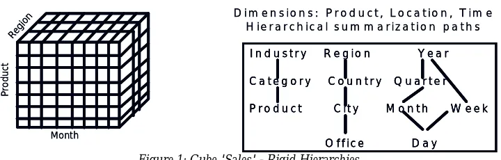
Figure 1: Cube 'Sales' - Rigid Hierarchies
A cubic structure [4] is defined as a 4-tuple <D, M, A, F> where the four components indicate the characteristics of the cube. These characteristics are:
• a set of n dimensions D = {d1,d2,…,dn} where each di is a dimension name,
extracted from a domain domdim(i).
• a set of k measures M = {m1,m2,…,mk} where each mi is a measure name,
extracted from a domain dommeasure(i).
• The set of dimension names and measures names are disjoint; i.e. D∩M=0.
• A set of t attributes A = {a1, a2,…,at} where each ai is an attribute name,
extracted from a domain domattr(i).
• A one-to-many mapping F:DàA, i.e. there exists, corresponding to each dimension, a set of attributes.
1.1.1 Semantics of the IF-Cube
In contrast, an IF-Cube is an abstract structure that serves as the foundation for the multidimensional data cube model. Cube C is defined as a five-tuple (D, l, F, O, H) where:
• D is a set of dimensions
• l is a set of levels l1,…, ln,
• A dimension di = (l ≤ O, l┴, l┬) dom(di) where l = li i=1...n.
• li is a set of values and li ∩ lj = {},
• ≤ O is a partial order between the elements of l.
• To identify the level l of a dimension, dl is used as part of a hierarchy. l┴: base level l┬: top level
for each pair of levels li and lj there exist the relation: μij : li × lj à [0,1] νij : li × lj à [0,1] 0 < μij + νij < 1
• F is a set of fact instances with schema: F = {<x, μF(x) , νF(x)>| x∈ X }, where x=<att1,…,attn> is an ordered tuple belonging to a given universe X, μF(x) and νF(x) are the degree of membership and non-membership of x in the fact table F respectively.
• H is an object type history that corresponds to a cubic structure (l, F, O, H′) which allows the tracing back the evolution of a cubic structure after performing a set of operators i.e. aggregation.
P
ro
d
uct
Regi on
Month
P
ro
d
uct
Regi on
Month
D i m e n s io n s : P r o d u c t , L o c a t io n , T im e H ie r a r c h ic a l s u m m a r iz a t i o n p a t h s
I n d u s t r y R e g io n Y e a r
C a t e g o r y C o u n t r y Q u a r t e r
P r o d u c t C it y M o n t h W e e k
O f f ic e D a y
D i m e n s io n s : P r o d u c t , L o c a t io n , T im e H ie r a r c h ic a l s u m m a r iz a t i o n p a t h s
I n d u s t r y R e g io n Y e a r
C a t e g o r y C o u n t r y Q u a r t e r
P r o d u c t C it y M o n t h W e e k
O f f ic e D a y I n d u s t r y R e g io n Y e a r
C a t e g o r y C o u n t r y Q u a r t e r
P r o d u c t C it y M o n t h W e e k
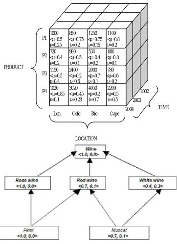
The example below provides a sample imprecise cube (D, l, F, O, H) i.e. sales and a conceptual flexible hierarchy product with reference to wine consisting of li,…,ln levels with respective levels of membership and non membership < μij νij, > .
PRODUCT
TIME
LOCATION
2003 Lon
P4 P3
1000
850 1250 1100
<μ=0.5 <μ=0.75 <μ=0.75 <μ=0.8
ν=0.25 ν=0.2 ν=0.15 ν=0.2
720 980 530 680
<μ=0.4 <μ=0.5 <μ=0.4 <μ=0.8
ν=0.2 ν=0.1 ν=0.2 ν=0.1
1150 2400 2000 780
<μ=0.5 <μ=0.2 <μ=0.7 <μ=0.6
ν=0.4 ν=0.6 ν=0.1 ν=0.2
1020 3020 4050 2200
<μ=0.85 <μ=0.45 <μ=0.2 <μ=0.5
ν=0.1 ν=0.28 ν=0.7 ν=0.5
P2 P1
Oslo Rio Cape 2004
2002
Figure 2: Imprecise cube 'Sales' Figure 3: H- IFS Hierarchy 'Wine’
The defined IF OLAP Cube and the proposed OLAP operators make it possible to do the following:
• accommodate imprecise facts.
• utilize conceptual hierarchies defined as H-IFS used for aggregation purposes in the cases of roll-up and roll-down operations.
• offer a unique feature such as keeping track of the history when there is movement between different levels of a hierarchical order.
In the next section, first the current cubic operators are reviewed and then the IF-Operators are explained. These operators have been extended and redefined in order to cope with or multidimensional model.
1.2 IF-cubic operators vs. normal cubic operators
process imprecise information. In the subsections below, first the original operators will be shown and then the new IF-Operators presented, which will be able to deal with the new multidimensional structure.
1.2.1 Overview of the cubic operators
The cubic model proposed in [4], which is considered by many OLAP experts to be the fundamental one when it comes to the cubic model, also describes the algebraic operators necessary for the functioning of the multidimensional cube that have been adopted widely. Below is shown a brief description of these operators, the full descriptions of which can be found on [4].
Restriction (σ): This operator restricts the values on one or more dimensions. It has an atomic predicate, denoted by p, that is a logical expression involving a single dimension or a compound predicate, denoted by P the is an expression involving a set of atomic predicates.
Mathematical notation: σp(Ci)=Co Example: σ(year=2009) (Sales)
Aggregation (α): This operator performs aggregation on one or more dimensions. This operator is based on relational aggregate functions (e.g. SUM AVG MAX) and allows these functions to be applied to cubes with one or more dimensions specified as grouping attributes.
Mathematical notation: α h,m, S (CI)=CO Example: α [SUM(amount),{product_name, year}](Sales)
Cartesian product (×): This is a binary operator that can be used to relate two cubes.
Mathematical notation: CI1 × CI2 = CO
Join (|×|): The join operator is a special case of the Cartesian product operator that is used to relate two cubes having one or more dimensions in common and having identical mapping from the common dimensions to the respective attribute sets of these dimensions.
Mathematical notation:: C1 |×| C2 = σp(C1×C2) where p is the predicate and C1and C2 are the two cubes.
Union (∪ ): This operator finds the union of two input cubes. If, for example, two cubes Sales_Engand and Sales_Wales contain the sales figures corresponding to the respective regions, and the user would like to consolidate the data for both regions into a single cube. This would be achieved by using the union operator.
Mathematical notation: CI1 ∪ CI2 = CO
Mathematical notation: CI1 - CI2 = CO
1.2.2 The IF-cubic operators
In this section the IF-Cubic operators are defined and explained. Each operator is presented in the following format: the operator’s name, symbol, textual description, input, output, mathematical description and an example of the operator.
Basic operators
Selection (Σ): The selection operator selects a set of fact-instances from a cubic structure that satisfy a predicate (θ). A predicate (θ) involves a set of atomic predicates (θ1, …, θn) associated with the aid of logical operators p (i.e. ∧,
∨, etc.). Only the cells that satisfy the predicate p are captured into the result cube. If θ’ is an Intuitionistic fuzzy predicate, then the set of possible facts that satisfy the θ should carry a degree of membership μ and non-membership ν expressed as follows:
F = {<x, min(μF(x), μ(θ(x))), max(νF(x), ν(θ(x))))> | x∈ X }
Thus the resulting cube populated with fact instances that either satisfy the predicate (θ) completely or to some degree of certainty. Whereπ = 1 – (μ + ν) and acts as an index of the uncertainty, i.e. the higher the value of π, the more uncertain the fact instance is, even though it may entail the same level of membership μ.
Input: Ci = (D, l, F, O, H) and the predicate θ. Output: Co= (D, l, Fo, O, H),where
Fo⊆ F and Fo={f | (f ∈F)∧(f satisfies θ)}.
Mathematical notation:
∑
θ(
C
i)
=
C
o.
Example: Find the sales amount of 1000 with membership of greater than 0.4 and non-membership of less than 0.3 for all products in all cities during 2004:4
Σ(amount=1000 ∧ (μ>0.4 ∧ν<0.3) ∧ year=2004 )(Sales)=CResult
Cubic Projection (Π): In cubic instances that hold non-deterministic facts, there can be no projecting-out of any of individual domains. The reason behind this statement is that unlike deterministic cubes, in non-deterministic ones the membership and non-membership of a fact instance determines the likelihood of all domains involved in that cube/fact instance. Hence, projecting out a domain, would result in loss of information.
Input: Ci = (D, l, F, O, H). Output: Co= (D, l, F, O, H).
Mathematical notation: ΠF (Ci) = Co.
Example: Project the cube from the previous example:
Basic Cubic Product (⊗): This is a binary operator Ci1⊗ Ci2. It is used to relate two cubes Ci1and Ci2 assuming that D1 ⊆ D2and O1, O2 are reconcilable
partial orders. Thus, l1, l2 could lead to 1o being a ragged hierarchy.
Input: Ci1 = (D1, l1, F1, O1, H1)and Ci2 = (D2, l2, F2, O2, H2).
Output: Co= (Do, lo, Fo, Oo, Ho),where
Do= D1∪D2, lo= l1∪l2, Oo= O1∪O2, Ho= H1∪H2,
Fo= F1×F2 ={<<x, y>,min(μf1(x), μf2(y)), max(νf1(x), νf2(y))> |<x, y> ∈X×Y}.
Mathematical notation: Ci1⊗Ci2 = Co.
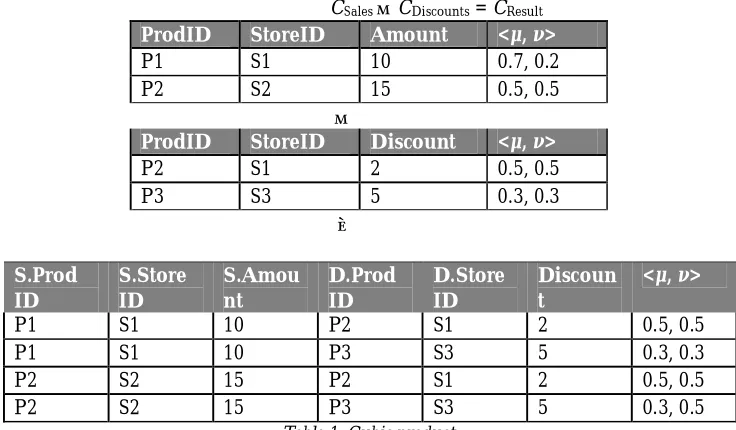
Example: Consider the two cubes one wants to relate, Ci1: CSales and Ci2: CDiscounts.
CDiscounts has the same dimensions as CSales except the measure amount is not
sale but is a discount. In that case the cubic product of these two, would be: CSales ⊗CDiscounts = CResult
ProdID StoreID Amount <μ, ν>
P1 S1 10 0.7, 0.2
P2 S2 15 0.5, 0.5
⊗
ProdID StoreID Discount <μ, ν>
P2 S1 2 0.5, 0.5
P3 S3 5 0.3, 0.3
⇓
S.Prod ID
S.Store ID
S.Amou nt
D.Prod ID
D.Store ID
Discoun t
<μ, ν>
P1 S1 10 P2 S1 2 0.5, 0.5
P1 S1 10 P3 S3 5 0.3, 0.3
P2 S2 15 P2 S1 2 0.5, 0.5
P2 S2 15 P3 S3 5 0.3, 0.5
Table 1: Cubic product
Union (∪ ): The union operator is a binary operator that finds the union of two cubes. Ci1 and Ci2 have to be union compatible. The operator also coalesces the value-equivalent facts using the minimum membership and maximum non-membership.
Input: Ci1 = (D1, 11, F1, O1, H1)and Ci2 = (D2, l2, F2, O2, H2).
Output: Co= (Do, lo, Fo, Oo, Ho),where
Do = D1 = D2, lo= l1 = l2,
Oo= O1 = O2, Ho= H1= H2,
Fo= F1∪ F2 =
={<x,max(µF1(x),µF2(x)),min(νF1(x),νF2(x))> | x ∈ X}.
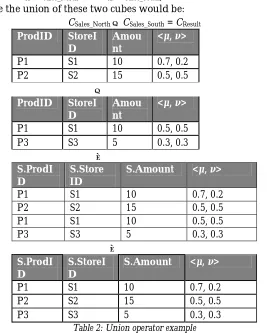
Example: Consider the two cubes one want to relate, Ci1: CSales_North and Ci2: CSales_South,
in that case the union of these two cubes would be: CSales_North ∪CSales_South = CResult
ProdID StoreI
D
Amou nt
<μ, ν>
P1 S1 10 0.7, 0.2
P2 S2 15 0.5, 0.5
∪
ProdID StoreI
D
Amou nt
<μ, ν>
P1 S1 10 0.5, 0.5
P3 S3 5 0.3, 0.3
⇓
S.ProdI D
S.Store ID
S.Amount <μ, ν>
P1 S1 10 0.7, 0.2
P2 S2 15 0.5, 0.5
P1 S1 10 0.5, 0.5
P3 S3 5 0.3, 0.3
⇓
S.ProdI D
S.StoreI D
S.Amount <μ, ν>
P1 S1 10 0.7, 0.2
P2 S2 15 0.5, 0.5
P3 S3 5 0.3, 0.3
Table 2: Union operator example
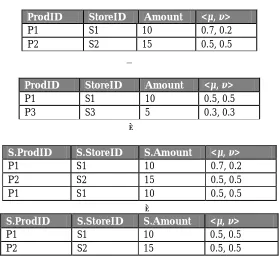
Difference (-): The difference operator is a binary operator that the difference of two cubes. It is similar to the difference operator in relational algebra. Ci1 and Ci2 have to be union compatible. The difference operator removes the portion of the cube Ci1 that is common to both cubes.
Input: Ci1 = (D1, l1, F1, O1, H1)and Ci2 = (D2, l2, F2, O2, H2).
Output: Co = (Do, lo, Fo, Oo, Ho), where
Do = D1 = D2, lo = l1 = l2, Oo= O1 = O2,
Ho= H1= H2,
Fo= F1∩ F2 = {<x, min(µF1(x),µF2(x)), max(νF1(x),νF2(x))> | x∈X}.
Mathematical notation: Ci1– Ci2 = Co.
Example: Consider the two cubes one wants to relate, Ci1: CSales_North and Ci2: CSales_South,
CSales_North – CSales_South = CResult
ProdID StoreID Amount <μ, ν>
P1 S1 10 0.7, 0.2
P2 S2 15 0.5, 0.5
_
ProdID StoreID Amount <μ, ν>
P1 S1 10 0.5, 0.5
P3 S3 5 0.3, 0.3
⇓
S.ProdID S.StoreID S.Amount <μ, ν>
P1 S1 10 0.7, 0.2
P2 S2 15 0.5, 0.5
P1 S1 10 0.5, 0.5
⇓
S.ProdID S.StoreID S.Amount <μ, ν>
P1 S1 10 0.5, 0.5
P2 S2 15 0.5, 0.5
Table 3: Difference operator example
Extended Operators
Join (Θ): The join operator relates two cubes having one or more dimensions in common, and having identical mappings from common dimensions to the respective attribute sets of these dimensions. This operation can be expressed using Cubic Product operation.
Ci1 = (D1, l1, F1, O1, H1)and Ci2 = (D2, l2, F2, O2, H2) are candidates to join if D1 ∩
D2≠ 0.
Input: Ci1 = (D1, 11, F1, O1, H1)and Ci2 = (D2, l2, F2, O2, H2).
Output: Co= (Do, lo, Fo, Oo, Ho).
Mathematical notation: Ci1 ΘCi2 = σp(Ci1⊗ Ci2).
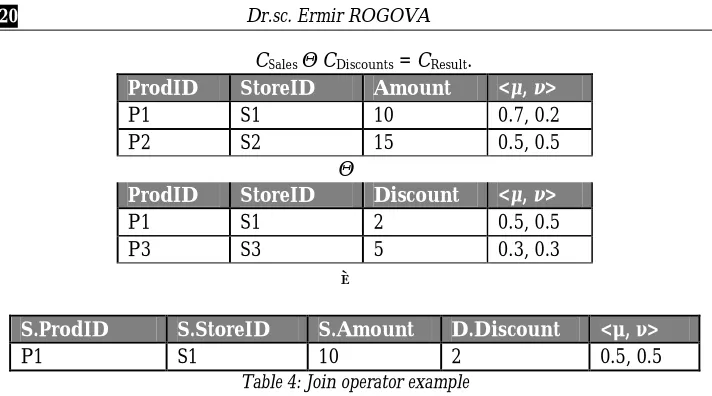
Example: Consider the two cubes one wants to relate, Ci1: CSales and Ci2:
CDiscounts. CDiscounts has the same dimensions as CSales except the measure amount
is not sale but is a discount.
CSales ΘCDiscounts = CResult.
ProdID StoreID Amount <μ, ν>
P1 S1 10 0.7, 0.2
P2 S2 15 0.5, 0.5
Θ
ProdID StoreID Discount <μ, ν>
P1 S1 2 0.5, 0.5
P3 S3 5 0.3, 0.3
⇓
S.ProdID S.StoreID S.Amount D.Discount <μ, ν>
P1 S1 10 2 0.5, 0.5
Table 4: Join operator example
Aggregation (A): The aggregation operator performs aggregation on one or more dimensional attributes utilizing Intuitionistic Fuzzy functions such as IFSSUM, IFSAVG, IFSMIN, IFSMAX. An aggregation operator A is a function A(G), where G = {<x, μF(x), νF(x)>| x∈ X},where x=<att1, …, attn> is an ordered tuple,
belonging to a given universe X, {att1, …, attn} is the set of attributes of the
elements of X, μF(x) and νF(x) are the degree of membership and non-membership of x.
The result is a bag of the type {<x′, μF(x′), νF(x′)> | x′∈ X}.To this extent, the bag is a group of elements that can be duplicated and each one has a degree of μ and ν.
Input: Ci = (D, l, F, O, H) and the function A(G). Output: Co = (D, lo,Fo, Oo, Ho).
The definition of aggregation operator points to the need of defining the IFS extensions for traditional group operators such as SUM, AVG, MIN and MAX.
Group Operations & Operators
In this section an investigation is made on how traditional group operations can be redefined to cope with the IFS representation of data. Note that the introduction of the IF facts influence the evaluation of aggregates at different levels:
• Will the result over which the aggregate is performed be either crisp or Intuitionistic Fuzzy?
• What is the meaning of the result after the IF aggregation is performed? Using the standard definitions for the group operators (SUM, AVG, MIN and MAX) as foundations, their IF extensions and meaning is provided.
with 1 ≤ i ≤ m. The fact instances fi are assumed to take Intuitionistic fuzzy values for the attribute attn-1 for i = 1to m
fi [attn-1] = {<μi(uki), νi(uki)>/ uki | 1 ≤ki ≤n}.
The IFSsumof the attribute attn-1of the fact table F is defined by:
≤ ≤ ∀ = ∧ = > < = =
∑
= = − )) ,..., 1 : ,..., ( )) ( ), ( ( min (( | / )) )( (( 1 1 1 1 1 n k k k k u y u u u y u F att IFS m m km k k ki ki i ki i m i n SUM i ν µIFSAVG : The IFSAVG aggregate, like its standard counterpart, is only defined for numeric domains. This aggregate makes use of the IFSSUM that was discussed previously and the standard COUNT. The IFSAVG can be defined as:
IFSAVG((attn-1)(F) = IFSSUM((attn-1)(F)) / COUNT((attn-1)(F)).
IFSMAX : The IFSMAX aggregate, like its standard counterpart, is only defined for numeric domains. Given a fact F defined on the schema X(att1, …,attn), let at
n-1 defined on the domain U={u1, …, un). The fact F consists of fact instances fi
with 1 ≤ i ≤ m. The fact instances fi are assumed to take intuitionistic fuzzy values for the attribute attn-1 for i = 1 to m
fi[attn-1] = {<μi(uki), νi(uki)>/ uki | 1 ≤ki ≤n}.
The IFSsumof the attribute attn-1of the fact table F is defined by:
(
)
{
/ |(( min ( ( ), ( )) max ( ( ), ( ))( ,..., :1 ,..., ))}
)) )( (( 1 1 1 1 1 n k k k k u u y u u u y u F att IFS m m ki i ki i m i ki i ki i m i n MAX ≤ ≤ ∀ = ∧ = > < = + = = − ν µ ν µ
IFSMIN: The IFSMIN aggregate, like its standard counterpart, is only defined for numeric domains. Given a fact F defined on the schema X(att1, …,attn), let
attn-1 defined on the domain U={u1, …, un). The fact F consists of fact instances fi
with 1 ≤ i ≤ m. The fact instances fi are assumed to take intuitionistic fuzzy values for the attribute attn-1 for i = 1 to m therefore fi[attn-1] = {<μi(uki), νi(uki)>/
uki | 1 ≤ki≤n}. The IFSsumof the attribute attn-1of the fact table F is defined by:
(
)
{
/ |(( min ( ( ), ( )) min ( ( ), ( ))( ,..., :1 ,..., ))}
)) )( (( 1 1 1 1 1 n k k k k u u y u u u y u F att IFS m m ki i ki i m i ki i ki i m i n MIN ≤ ≤ ∀ = ∧ = > < = = = = − ν µ ν µ
It can be observed that the IFSMIN is extended in the same manner as IFSMAX aggregate except for replacing the symbol max in the IFSMAX definition with
min.
The definition of the extended group operations makes it possible to define the extended group operators Roll up (∆), and Roll Down (Ω).
Roll up (∆): The result of applying Roll up over dimension di at level dlr using
the aggregation operator A over a datacube Ci = (Di, li, Fi, O, Hi) is another datacube Co = (Do, lo, Fo, O, Ho).
Output: Co = (Do, lo, Fo, O, Ho).
An object of type history is a recursive structure:
H =
{
ω is the initial state of the cube
(l, D, A, H’) is the state of the cube after performing an operation on the cube
The structured history of the datacube allows the storing of all the information when applying Roll up and the recall of it back when Roll Down is performed. In order to be able to apply the operation of Roll Up the IFSSUM aggregation operator needs to be put to use.
Roll Down (Ω): This operator performs the opposite function of the Roll Up operator. It is used to roll down from the higher levels of the hierarchy with a greater degree of generalization, to the leaves with the greater degree of precision. The result of applying Roll Down over a datacube Ci = (D, l, F, O, H) having H= (l’, D’, A’, H’) is another datacube Co= (D’, l’, F’, O, H’).
Input: Ci = (D, l, F, O, H).
Output: Co = (D’, l’, F’, O, H’) where F’à set of fact instances defined by
operator A.
To this extent, the Roll Down operative makes use of the recursive history structure previously created after performing the Roll Up operator.
1.3 Conclusions
In this paper the context of value imprecision was revised, as part of an MOLAP based environment. A new approach for extending the MOLAP model was presented, so that it can include treatment of value uncertainty as part of a multidimensional model, inhabited by concepts and flexible hierarchical structures of organization. A new multidimensional-cubic model named the IF-Cube was introduced, which is able to operate over data with imprecision either in the facts or in the dimensional hierarchies.
The main contribution of this new multidimensional-cubic model is that is able to operate over data with imprecision in the facts and the summarisation hierarchies. Classical models imposed a rigid structure that made the models present difficulties when merging information from different but still reconcilable sources.
References:
1. R. Kimball, The Data Warehouse Toolkit. New York, John Wiley & Sons, 1996. 2. S. Chaudhuri, U. Dayal, V. Ganti Database Technology for Decision Support
Systems. In: Computer, Vol. 34, p. 48-55, 2001
3. M. Jarke, Fundamentals of data warehouses. Springer, London, 2002
4. H. Thomas & A. Datta, A Conceptual Model and Algebra for On-Line Analytical Processing in Decision Support Databases. Information Systems Research 12: pp.83-102, 2001
5. C. Dyreson, Information retrieval from an incomplete data cube, VLDB, Morgan Kaufman Publishers, pp. 532-543, 1996.
6. T. Pedersen, C. Jensen, and C. Dyreson, A foundation for capturing and querying complex multidimensional data, Information Systems, vol. 26, pp. 383-483, 2001. 7. E. Rogova, P. Chountas, On Imprecision Intuitionistic Fuzzy Sets & OLAP – The
Case for KNOLAP, IFSA’07, Springer-Verlag GmBh , Theoretical advances and application of fuzzy logic and soft computing, pp. 11-20
8. E. Rogova, P. Chountas, B. Kolev, Intuitionistic Fyzzy Knowledge-based OLAP, Notes on Intuitionistic Fuzzy sets, Vol. 13, No.2, ISSN 1310-4926, 2007, pp.88-100 9. K. Atanassov (1999). Intuitionistic Fuzzy Sets, Springer-Verlag, Heidelberg