A simulation-based robust biofuel facility location model for an integrated bio-energy logistics network

(1)

JIEM, 2014 – 7(5): 1415-1432 – Online ISSN: 2013-0953 – Print ISSN: 2013-8423 http://dx.doi.org/10.3926/jiem.1196

A Simulation-Based Robust Biofuel Facility Location Model

for an Integrated Bio-Energy Logistics Network

Jae-Dong Hong

1

_{, Keli Feng}

1

_{, Yuanchang Xie}

2

1

_{South Carolina State University (United States)}

2

_{University of Massachusetts Lowell (United States)}

[email protected], [email protected], [email protected]

Received: June 2014

Accepted: November 2014

Abstract:

Purpose:

The purpose of this paper is to propose a simulation-based robust biofuel facility

location model for solving an integrated bio-energy logistics network (IBLN) problem, where

biomass yield is often uncertain or difficult to determine.

Design/methodology/approach:

The IBLN considered in this paper consists of four

different facilities: farm or harvest site (HS), collection facility (CF), biorefinery (BR), and

blending station (BS). Authors propose a mixed integer quadratic modeling approach to

simultaneously determine the optimal CF and BR locations and corresponding biomass and

bio-energy transportation plans. The authors randomly generate biomass yield of each HS and

find the optimal locations of CFs and BRs for each generated biomass yield, and select the

robust locations of CFs and BRs to show the effects of biomass yield uncertainty on the

optimality of CF and BR locations. Case studies using data from the State of South Carolina in

the United State are conducted to demonstrate the developed model’s capability to better

handle the impact of uncertainty of biomass yield.

(2)

investments, and would assist potential investors in identifying the least cost or important

facilities to invest in the biomass and bio-energy industry.

Originality/value:

An optimal biofuel facility location model is formulated for the case of

deterministic biomass yield. To improve the robustness of the model for cases with

probabilistic biomass yield, the model is evaluated by a simulation approach using case studies.

The proposed model and robustness concept would be a very useful tool that helps potential

biofuel investors minimize their investment risk.

Keywords:

bio-energy logistics network, robust biorefinery location, biomass yield, simulation

approach

1. Introduction

Diverse and affordable energy is critical for the future of every country in the world. To reduce the dependence on foreign oil and also mitigate the environmental impacts (e.g., climate change, pollution) of using fossil fuel, a significant amount of research in the United States has recently been devoted to methods of producing biofuel. Less attention has been given to the cost of transporting bulky biomass feedstock to biorefinery plants. The biomass transportation cost is, however, significant compared to the biofuel production cost. For this reason, a majority of existing biorefinery plants in the United States are located in the Midwest where biomass, such as corn and soybean, is abundant.

With the soaring and unstable gasoline price and the increasing environmental concern, many other states in the U.S. are now seeking the opportunity to use biomass feedstocks, such as switchgrass, for producing biofuel. Also, under the Energy Independence and Security Act (EISA) of 2007, the United States Environmental Protection Agency (EPA) has developed a Renewable Fuel Standard Program (RFS) to ensure that gasoline in the U.S. contains a minimum percentage of renewable fuel. The latest RFS (2011) “will increase the volume of renewable fuel required to be blended into gasoline from 9 billion gallons in 2008 to 36 billion gallons by 2022.” Therefore, there is an immediate demand for biomass transportation cost analysis model to help locate new biorefineries optimally.

(3)

scale BRs working on novel refining processes, and more than $400 million for bio-energy centers (2011).

The vast expansion in biofuels production and use mandated by EISA will require the development of new methods and equipment to collect, store, and pre-process biomass in a manner acceptable to biorefineries. These activities, which constitute as much as 20% of the current cost of finished cellulosic ethanol, are comprised of four main elements:

• Harvesters & collectors that remove feedstocks from cropland and out of forests.

• Storage facilities that provide a steady supply of biomass to the biorefinery, in a manner that prevents material spoilage.

• Preprocessing/grinding equipment that transforms feedstocks to the proper moisture content, bulk density, viscosity, and quality.

• Transportation of feedstocks and biofuels

(4)

Figure 1. Schematic of Biomass/Bio-Energy Logistics Network

What complicates the decision of CF and BR locations is the uncertainty in biomass yield. Intuitively, different biomass yield scenarios will affect the optimality of a biofuel facility location plan. To develop a robust model, we first present a mixed integer quadratic program (MIQP) modeling approach to simultaneously determine the optimal locations of BRs and CFs and the transportation scheme for a given biomass yield scenario. We then investigate the effects of biomass yield on the optimality of the selected location by simulating the biomass yield of each HS, i.e., generating biomass yield for each HS using three probability distributions and finding the optimal locations of BRs and CFs for each yield scenario. Based on the simulation results, we identify the most frequently selected locations of BRs and CFs (referred to as ‘robust locations’,) for various biomass yields scenarios. By comparing the optimal solutions for the different biomass yield scenarios, a robust location is then identified.

2. Literature Review

Many existing studies have focused on bio-processing technologies to improve the biofuel yield and quality (Antonpoulou, Gavala, Skiadas, Angelopoulos & Lyberatos, 2008; Lee, Chou, Ham, Lee & Keasling, 2008; Ranganathan, Narasimhanm & Muthukumar, 2008; van Dyken, Bakken & Skjelbred, 2010; Weyens, Lelie, Taghavi, Newman & Vangronsveld, 2009). Although the cost of transporting bulky and unrefined biomass feedstock is also significant as compared to the total cost for producing biofuel, much less attention has been given to the understanding of biomass and bio-energy logistics systems and the reduction of biomass and bio-energy logistics costs.

(5)

Perpiñá, Alfonso, Pérez-Navarro, Peñalvo, Vargas & Cárdenas, 2009; Steen, Kang, Bokinky, Hu, Schimer, McClure et al., 2010) or on the optimization and simulation of the biomass collection, storage, and transport operations (Frombo, Minciardi, Robba, Rosso & Sacile, 2009; Kumar & Sokhansanj, 2007; Rentizelas, Tolis & Tatsiopoulos, 2009; Sokhansanj, Kumar & Turhollow, 2006). Eksioglu, Acharya, Leightley and Arora (2009) investigate the integrated biomass and biofuel logistics network design, simultaneously taking into account the optimization of facility locations (e.g., collection facilities, biorefineries), transportation, and inventory control. In their paper, several critical issues are not adequately addressed: for instance, how the uncertainty in biomass yield affects the robustness and optimality of the logistics network design and how to develop efficient heuristic algorithms to solve the formulated logistics model, which typically is an NP-hard problem.

The remaining of the paper is organized as follows. Section 3 introduces an integrated facility location and transportation model in detail. Following the description of the model formulation, case studies are conducted and analysis for simulation results is presented in section 4. Section 5 summarizes the developed models and research findings. It also provides recommendations for future research directions.

3. Development of Integrated Optimization Model

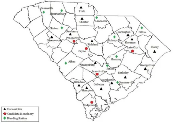
We propose the integrated optimization mathematical model by modifying the model (Eksioglu et al., 2009). In our proposed model, we assume that CFs can be located at any HS and a biorefinery (BR) can only be built at candidate BR location, since BR locations must satisfy some realistic requirements. This is a reasonable assumption at the planning stage for the bio-energy logistics model. It may be difficult to decide potential CF locations which are not HSs, since the assignment of HSs to a CF is not known.

Let F be the set of all harvesting sites (HSs) and potential collection facility (CF) locations, indexed by f. Now, let J, I, and K respectively be the set of CFs, BRs, and BSs, indexed by j, i, and k. Also, let L and G respectively be the set of capacities of BR and CF, indexed by l and g. The parameters used in this formulation are the following: is amortized annual cost of constructing and operating a BRi with the lt h size; is amortized annual cost of constructing

and operating a CFj with the gth size; and denote the actual capacity of lth and gth size of

BR and CF, respectively; βf and γf are conversion rates to bio-energy of biomass feedstock

shipped from CF to BR and from HS to BR, respectively; Sf denotes the yield of biomass

feedstock from HSf; Dk is the demand of biofuel for BSk; is the maximum number of HSs that

ship biomass directly to Bri; , , and are unit transportation cost (UTC) from HSf to

(6)

= * ,  ≥ 1 to denote a higher unit transportation cost for shipping biomass from HSf

directly to BRi.

The decision variables used in the mixed integer quadratic programming (MIQP) formulation are the following: is a binary variable that equals 1 if a biorefinery of size l is located in site

i, and 0 otherwise; is a binary variable that equals 1 if a collection facility of size g is located in site j, and 0 otherwise; is a binary variable that equals 1 if HSf’s yielded biomass

shipped to CFj and 0 otherwise; is a binary variable that equals 1 if HSf ships biomass

directly to BRi, and 0 otherwise; is a binary variable that equals to 1 if CFj is assigned to BRi,

and 0 otherwise; is the fraction of BRi’ produced biofuel shipped to BSk; is the fraction of

demand for BSk that must be satisfied by a dummy BRm, for the occurrence of shortage, that

is, the total demand of all BSs cannot be met because the total supply from all BRs is not enough, and 0 otherwise.

Letting Nb and Nc denote the maximum number of BRs and CFs to be built, we formulate the

following MIQP model that minimizes the total logistics cost (TLC), which is the sum of the annualized construction and operation cost for CFs and BRs and the transportation costs from HSs to CFs, HSs to BRs, CFs to BRs, and BRs to BSs:

(1)

(2)

(3)

(4)

(5)

(6)

(7)

(8)

(7)

(10)

(11)

(12)

(13)

Constraints (2) and (3) ensure that a BR and a CF of size l and g are located in sites i and j. Constraints (4) and (5) require that at most Nb BRs and Nc CFs can be constructed. Constraints

(6) ensure that each HS is assigned to a CF or a BR. Constraints (7) ensure that each selected CF should cover at least uj and at most uj HSs (set to 2 and 10 in this study). Constraints (8)

are capacity constraint for CFs, that is, the amount of biomass a CF receives should not exceed its capacity. Constraints (9) are capacity constraint for BRs, that is, the amount of biofuel a BR can produce should not exceed its capacity. Constraints (10) ensure that a CF supplies biomass to the selected BR sites only. Constraints (11) ensure that at most δi HS is directly covered by

BRi. Constraints (12) and (13) ensure that the total amount of biofuel converted from biomass

by all BRs is enough to satisfy the total demand of biofuel for all BSs. If not, a dummy biorefinery, BRm, is added to satisfy the shortage.

To solve the above MIQP problem, letting to linearize the term in Equations (1),

(9) and (11), we add the following:

(14)

Hereafter, this newly introduced model given by Equations (1)-(14) is referred to as the Integrated Biofuel Facility Location (IBFL) model.

4. Case Study

(8)

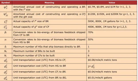
Although not shown in Figure 3, the actual distances among cities representing HSs, CFs, BRs, and BFs, are calculated. Table 1a shows the demands (in thousand gallons) for all BSs. These demands are hypothetical values and can be readily replaced by true demand data for real-world applications. The values of the input parameters are summarized in Table 1b. Based on these input data, an Excel Spreadsheet model is developed. Excel Analytic Solver Platform with VBA (Visual Basic for Applications) is used to solve the proposed model.

To simulate the uncertainty in biomass yields, we randomly generate biomass yield for each HS using three popular probability distributions. The minimum and maximum biomass yield values for each HS are obtained from the ranges shown in Figure 2. The probability distributions considered in this paper are normal distribution, uniform distribution, and triangular distribution.

(9)

Figure 3. Candidate Biorefinery, Harvesting Sites, and Blending Stations

No. Blending Station Demand(in 1000 gallons)

1 Aiken 300

2 Bishopville 200

3 Clinton 300

4 Dillon 150

5 Greenville 150

6 Lancaster 200

7 Manning 250

8 Santee 150

9 Spartanburg 300

10 Summerville 200

(10)

Symbol Meaning Value

Amortized annual cost of constructing and operating a BRi

with the lth _size $0.7M, $0.8M, and $1M for l=1, 2, 3.

Amortized annual cost of constructing and operating a CFj

with the gth size $120K, $150K, and $200K for g=1, 2, 3.

Actual capacity of lth_{size of BR} _{500K, 800K, 1M gallons for}_l_{=1, 2, 3.}

Actual capacity of gth_{size of CF} _{400K, 800K, 1M tons for g=1,2,3.}

βf Conversion rates to bio-energy of biomass feedstock shipped

from CF to BR 70%

γf Conversion rates to bio-energy of biomass feedstock shipped

from HS to BR 50%

δi Maximum number of HSs that ship biomass directly to BRi 1

Nb Maximum number of BRs to be built 3

Nc Maximum number of CFs to be built 6

Unit transportation cost (UTC) from HSfto CFj $0.08/mile/K metric tons

Unit transportation cost (UTC) from HSf to BR _2*

Unit transportation cost (UTC) from CFj to BRi $0.04/mile/K metric tons

Unit transportation cost (UTC) from BRi to BSk $0.01/mile/K gallons

Table 1b. Input Data Used for Case Study

Case 1. Normal Distribution: in this case, the mean biomass yield at HSf, μf, and its standard

deviation, σf, are obtained from

μf = (wf + Wf)/2 (15)

and

σf = (Wf – wf)/6 (16)

where wf and Wf denote minimum and maximum amounts of biomass yield at HSf shown in

Figure 2. To derive Equation (16), we assume that wf and Wf are located at three standard

deviations on either side of its mean.

Case 2. Uniform Distribution: we use the minimum, wf, and maximum value, Wf for the

parameters of the uniform distribution.

Case 3. Triangular Distribution: two skewed distributions are considered for biomass yield. The first one is a right-skewed distribution. Its mode, O(r)f, is located at

O(r)f = wf + (Wf – wf)/4 (17) The other one is a left-skewed distribution. Its mode, O(l)f, is located at

O(r)f = Wf – (Wf – wf)/4 (18)

For Equations (17) and (18), we assume that a mode is located at (Wf, – wf)/4 to the right side

of the minimum amount (wf) for the right-skewed distribution and to the left side of the

(11)

5. Numerical Results and Observations

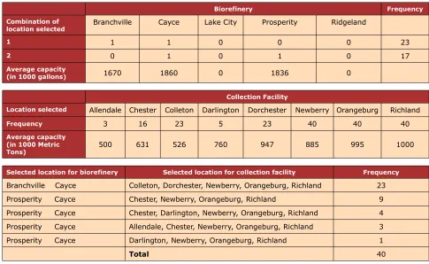
We assume shortage costs to be equal to zero, since the occurrence of biofuel shortage would not affect the optimal locations of BRs and CFs. We solve the developed model for forty (40) different sets of simulated biomass yields for each probability distribution and present the frequencies of BR and CF to be included in the optimal solutions in Tables 2a through 2d. ‘1’ for BR location columns in these tables denotes that this location is selected in the optimal solution and ‘0’ otherwise. For the case of normal distribution (see Table 2a), the frequencies for selected BR location set 1 {Branchville, Cayce} and BR location set 2 {Prosperity, Cayce} are 23 and 17, respectively, whereas for the case of uniform distribution, the frequencies for BR location set 1 {Branchville, Cayce} and BR location set 2 {Prosperity, Cayce} are exactly same (see Table 2b). However, for the skewed triangle distribution case, one BR location set is dominant over the other. For the right-skewed triangle distribution, the simulated biomass yields are more likely to be less than the middle value of wf and Wf. Due to this, the BR location

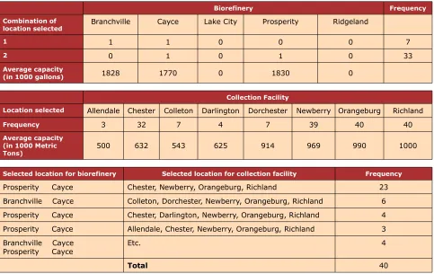
set 2 {Prosperity, Cayce} is selected more frequently (33 times out of 40) as shown in Table 2c, whereas the BR location set 1 {Branchville, Cayce} is selected more frequently (36 times out of 40) for the left-skewed distribution as shown in Table 2d.

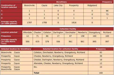
The selected locations of CFs depend upon the locations of BRs. As the results in Tables 2a through 2d and Table 3 suggest, when the BR location set 1 {Branchville, Cayce} is chosen, the CF location set {Colleton, Dorchester, Newberry, Orangeburg, Richland} is selected 83 times out of 86 (see Table 3). Given that the BR location set 2 {Prosperity, Cayce} is selected, the CF location set {Chester, Newberry, Orangeburg, Richland} is selected 39 times out of 73. The total capacity of these four (4) CF locations is sometimes insufficient. Therefore, the second most frequent CF location set, {Chester, Newberry, Orangeburg, Richland, Darlington} selected 16 times out of 17, is considered. From Table 3, we observe that two CF candidates, {Orangeburg, Richland}, are always selected regardless of the types of distribution or the selected BR locations. Another candidate CF location, {Newberry}, is selected 158 times out of 160. From now on, we refer to the location {(Branchville, Cayce), (Colleton, Dorchester, Newberry, Orangeburg, Richland)} as ‘Robust Location 1’ and {(Prosperity, Cayce), (Chester, Newberry, Orangeburg, Richland, Darlington)} as ‘Robust Location 2,’ respectively.

To evaluate the efficiency of Robust Locations 1 and 2, we consider the following extreme scenarios:

Scenario I: Each HS yields the minimum amount of biomass, wf,  f  F.

Scenario II: Each HS yields the middle amount of biomass, (wf, + Wf)/2,  f  F.

(12)

Biorefinery Frequency

Combination of

location selected Branchville Cayce Lake City Prosperity Ridgeland

1 1 1 0 0 0 23

2 0 1 0 1 0 17

Average capacity

(in 1000 gallons) 1670 1860 0 1836 0

Collection Facility

Location selected Allendale Chester Colleton Darlington Dorchester Newberry Orangeburg Richland

Frequency 3 16 23 5 23 40 40 40

Average capacity (in 1000 Metric

Tons) 500 631 526 760 947 885 995 1000

Selected location for biorefinery Selected location for collection facility Frequency

Branchville Cayce Colleton, Dorchester, Newberry, Orangeburg, Richland 23

Prosperity Cayce Chester, Newberry, Orangeburg, Richland 9

Prosperity Cayce Chester, Darlington, Newberry, Orangeburg, Richland 4

Prosperity Cayce Allendale, Chester, Newberry, Orangeburg, Richland 3

Prosperity Cayce Darlington, Newberry, Orangeburg, Richland 1

Total 40

Table 2a. Simulation Results of Locations of Biorefinery and Collection Facility for Case 1 (Normal Distribution)

Combination of

1 1 1 0 0 0 20

2 0 1 0 1 0 20

(in 1000 gallons) 1760 1830 0 1780 0

Frequency 5 20 19 6 20 39 40 40

Tons) 500 590 579 500 920 895 995 1000

Branchville Cayce Colleton, Dorchester, Orangeburg, Richland 2

Prosperity Cayce Etc. 2

Total 40

(13)

Combination of

1 1 1 0 0 0 7

2 0 1 0 1 0 33

(in 1000 gallons) 1828 1770 0 1830 0

Frequency 3 32 7 4 7 39 40 40

Tons) 500 632 543 625 914 969 990 1000

Branchville Cayce

Prosperity Cayce Etc. 4

Total 40

Table 2c. Simulation Results of Locations of Biorefinery and Collection Facility for Case 3 (Right-Skewed Triangle Distribution)

Combination of

1 1 1 0 0 0 36

2 0 1 0 1 0 3

3 1 0 0 1 0 1

(in 1000 gallons) 1870 1734 0 1800 0

Frequency 1 3 37 2 37 40 40 40

Tons) 500 600 616 500 978 820 995 995

Branchville Prosperity Colleton, Dorchester, Newberry, Orangeburg, Richland 1

Total 40

(14)

Combination of

1 1 1 0 0 0 86

2 0 1 0 1 0 73

3 1 0 0 1 0 1

(in 1000 gallons) 1787 1799 0 1816 0

Frequency 12 71 86 17 87 158 160 160

Tons) 500 619 578 556 961 861 995 997

Prosperity Cayce

Branchville Cayce Etc. 10

Total 160

Table 3. Summary of Simulation Results of Locations of Biorefinery and Collection Facility

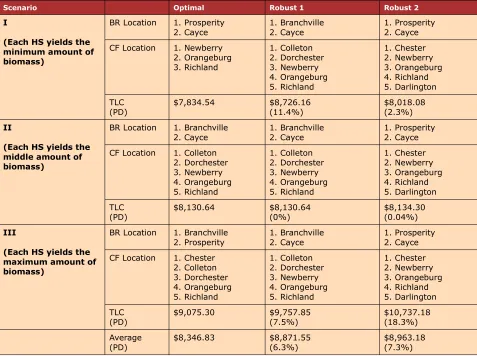
In Table 4, we compare the optimal solutions of each simulated biomass yield scenario with Robust Location 1 and Robust Location 2. We also report the percentage deviation (PD) of Robust 1 and Robust 2 from the optimal solution for each scenario. As expected from Tables 2 and 3 and seen in Table 4, for Scenario I, which is an extreme case of the right skewed distribution, Robust 2 performs better than Robust 1. For Scenario III, an extreme case of the left skewed distribution, Robust 1 outperforms Robust 2. For Scenario II, both Robust 1 and Robust 2 perform well compared to the optimal solution, since the PDs yielded by Robust 1 and Robust 2 are 0% and 0.04%. In terms of the maximum PD (MXPD) for all scenarios, Robust 1 with 11.4% performs better than Robust 2 with 18.3%. On the average of PD (AVPD), Robust 1 with 6.3% performs slightly better than Robust 2 with 7.3%, which is consistent with the results shown in Table 3.

6. Summary and Conclusions

(15)

Solver Platform with VBA (Visual Basic for Applications). For the biomass and bio-energy logistics network, the uncertainty in biomass yield has been a critical factor for determining the optimal locations of BRs and CFs, since it significantly affects the logistics network operational costs. To demonstrate the developed model’s capability and to evaluate the effects of the uncertainty in biomass yield, a case study is conducted using the data from United States EPA as shown in Figure 2. We simulate the biomass yield uncertainty by randomly generating biomass yield for each HS using normal, uniform, and triangular probability distributions. We then find the optimal locations of BRs and CFs for each generated set of biomass yield data.

Scenario Optimal Robust 1 Robust 2

I

(Each HS yields the minimum amount of biomass)

BR Location 1. Prosperity

2. Cayce 1. Branchville2. Cayce 1. Prosperity2. Cayce

CF Location 1. Newberry

2. Orangeburg 3. Richland 1. Colleton 2. Dorchester 3. Newberry 4. Orangeburg 5. Richland 1. Chester 2. Newberry 3. Orangeburg 4. Richland 5. Darlington TLC

(PD) $7,834.54 $8,726.16(11.4%) $8,018.08(2.3%)

II

(Each HS yields the middle amount of biomass)

BR Location 1. Branchville

2. Cayce 1. Branchville2. Cayce 1. Prosperity2. Cayce

CF Location 1. Colleton

2. Dorchester 3. Newberry 4. Orangeburg 5. Richland 1. Colleton 2. Dorchester 3. Newberry 4. Orangeburg 5. Richland 1. Chester 2. Newberry 3. Orangeburg 4. Richland 5. Darlington TLC

(PD) $8,130.64 $8,130.64(0%) $8,134.30(0.04%)

III

(Each HS yields the maximum amount of biomass)

BR Location 1. Branchville

2. Prosperity 1. Branchville2. Cayce 1. Prosperity2. Cayce

CF Location 1. Chester

2. Colleton 3. Dorchester 4. Orangeburg 5. Richland 1. Colleton 2. Dorchester 3. Newberry 4. Orangeburg 5. Richland 1. Chester 2. Newberry 3. Orangeburg 4. Richland 5. Darlington TLC

(PD) $9,075.30 $9,757.85(7.5%) $10,737.18(18.3%)

Average

(PD) $8,346.83 $8,871.55(6.3%) $8,963.18(7.3%)

*PD stands for percentage deviation, (TLC yielded by Robust location – Optimal TLC)/Optimal TLC

Table 4. Comparison between Results of Optimal and Robust Locations

(16)

Thus, the model developed in this paper would help decision-makers find the robust locations of biorefinery and collection facility, which require huge investments, and would assist the potential investors in identifying the most profitable or important facilities to invest in the biomass and bio-energy industry. This model could be a very useful tool that helps them minimize the investment risk.

For future research, it would be necessary to consider truck routing for collecting less-than-truckload biomass from farms, as this very likely could lead to improved transportation efficiency in the biomass collection process.

Acknowledgement

This research is supported by the 1890 Institution Teaching, Research and Extension Capacity Building Grants of National Institute of Food Agriculture (NIFA), US Department of Agriculture, under Grant No. 2010-38821-21595.

References

Antonpoulou, G., Gavala, H. N., Skiadas, L.V., Angelopoulos, K., & Lyberatos, G. (2008). Biofuel generation from sweet sorghum: fermentative hydrogen production and anaerobic digestion of the remaining biomass. Bioresource Technology, 99(1), 110-119.

http://dx.doi.org/10.1016/j.biortech.2006.11.048

Celli, G., Ghiani, E., Loddo, M., Pilo, F., & Pani, S. (2008). Optimal location of biogas and biomass generation plants. In Proceedings of the 43rd International Universities Power Engineering Conference, Padova, Italy, 1-6.

Eksioglu, S.D., Acharya, A., Leightley, L.E., & Arora, S. (2009). Analyzing the design and management of biomass-to-biorefinery supply chain. Computers & Industrial Engineering, 57(4), 1342-1352. http://dx.doi.org/10.1016/j.cie.2009.07.003

EPA Tracked Sites in South Carolina with Biorefinery Facility Siting Potential (2013). Retrieved June 15, 2013, from www.epa.gov/renewableenergyland/maps/pdfs/biorefinery_sc.pdf.

(17)

Graham, R.L., English, B.C., & Noon, C.E. (2000). A Geographic Information System-based modeling system for evaluating the cost of delivered energy crop feedstock. Biomass and Bioenergy, 18(5), 309-329. http://dx.doi.org/10.1016/S0961-9534(99)00098-7

Kumar, A., & Sokhansanj, S. (2007). Switchgrass (Panicum vigratum, L.) delivery to a biorefinery using integrated biomass supply analysis and logistics (IBSAL) model. Bioresource Technology, 98(5), 1033-1044. http://dx.doi.org/10.1016/j.biortech.2006.04.027

Lee, S.K., Chou, H., Ham, T. S., Lee, T.S., & Keasling, J.D. (2008). Metabolic engineering of microorganisms for biofuel production: from bugs to synthetic biology to fuels. Current Opinions in Biotechnology, 19(6), 556-563. http://dx.doi.org/10.1016/j.copbio.2008.10.014

Panichelli, L., & Gnansounou, E. (2008). GIS-based approach for defining bioenergy facilities location: A case study in Northern Spain based on marginal delivery costs and resources competition between facilities. Biomass and Bioenergy, 32(4), 289-300.

http://dx.doi.org/10.1016/j.biombioe.2007.10.008

Perpiñá, C., Alfonso, D., Pérez-Navarro, A, Peñalvo, E., Vargas, C., & Cárdenas, R. (2009). Methodology based on Geographic Information Systems for biomass logistics and transport optimization. Renewable Energy, 34(3), 555-565. http://dx.doi.org/10.1016/j.renene.2008.05.047

Ranganathan, S.V., Narasimhanm, S.N., & Muthukumar, K. (2008). An overview of enzymatic production of biodiesel. Bioresource Technology, 99(10), 3975-3981.

http://dx.doi.org/10.1016/j.biortech.2007.04.060

Rentizelas, A.A., Tolis, A.J., & Tatsiopoulos, L.P. (2009). Logistics issues of biomass: The storage problem and the multi-biomass supply chain. Renewable and Sustainable Energy Reviews, 13(4), 887-894. http://dx.doi.org/10.1016/j.rser.2008.01.003

Sokhansanj, S., Kumar, A., & Turhollow, A.F. (2006). Development and implementation of integrated biomass supply analysis and logistics model (IBSAL). Biomass and Bioenergy, 30(10), 838-847. http://dx.doi.org/10.1016/j.biombioe.2006.04.004

Steen, E.J., Kang, Y., Bokinsky, G., Hu, Z., Schirmer, A., McClure et al., (2010). Microbial production of fatty-acid-derived fuels and chemicals from plant biomass. Nature, 43, 559-562. http://dx.doi.org/10.1038/nature08721

United States Environmental Protection Agency, Renewable Fuel Standard Program (2011). Retrieved, July 23, 2011, from http://www.epa/gov/otaq/fuels /renewablefuels/index.htm

van Dyken, S., Bakken, B.H., & Skjelbred, H.I. (2010). Linear mixed integer models for biomass supply chains with transport, storage and processing. Energy, 35 (3), 1338-1350.

(18)

Weyens, N., Lelie, D., Taghavi, S., Newman, L., & Vangronsveld, J. (2009). Exploiting plant-microbe partnerships to improve biomass production and remediation. Trends in Biotechnology, 27(10), 591-598. http://dx.doi.org/10.1016/j.tibtech.2009.07.006

Journal of Industrial Engineering and Management, 2014 (www.jiem.org)

Article's contents are provided on a Attribution-Non Commercial 3.0 Creative commons license. Readers are allowed to copy, distribute and communicate article's contents, provided the author's and Journal of Industrial Engineering and Management's names are included.