Optimal priority ordering in PHP production of multiple part-types in a failure-prone machine

(1)

doi:10.3926/jiem.2009.v2n3.p418-436 ©© JIEM, 2009 – 2(3): 418-436 - ISSN: 2013-0953

Optimal priority ordering in PHP production of multiple

part-types in a failure-prone machine

Ana Sánchez, Albert Corominas, Rafael Pastor

Universitat Politècnica de Catalunya (SPAIN)

Received March 2009

Accepted September 2009

Abstract: This note deals with the problem of minimising the expected sum of quadratic

holding and shortage inventory costs when a single, failure-prone machine produces

multiple part-types. Shu and Perkins (2001) introduce the problem and, by restricting the

set of control policies to the class of prioritised hedging point (PHP) policies, establish

simple, analytical expressions for the optimal hedging points provided that the priority

ordering of the part-types is given. However, the determination of an optimal priority

ordering is left by the authors as an open question. This leaves an embedded sequencing

problem which we focus on in this note. We define a lower bound for the problem,

introduce a test bed for future developments, and propose three dynamic programming

approaches (with or without the lower bound) for determining the optimal priority

orderings for the instances of the test bed. This is an initial step in a research project aimed

at solving the optimal priority ordering problem, which will allow evaluating the

performance of future heuristic and metaheuristic procedures.

(2)

1 Introduction and problem statement

Shu and Perkins (2001) introduce the problem of optimising the costs of a production system that consists in a single, failure-prone machine that is able to

produce up to

n

part-types simultaneously with constant demand rates

(

d

j

;

j

=

1,...,

n

)

. The machine alternately adopts an “up” state, in which it is fully

functional, and a “down” state, in which it is not able to produce anything. The time that the machine spends in each state before switching to the other is distributed exponentially with parameters equal to

1

q

_d and

1

q

_u for the “down”

and “up” states respectively. The vector of the production rates to be determined for each part-type in each instant of time

t

is

x t

( )

=

[

x t x t

₁

( ),

₂

( ),. . . ,( )

x t

_n

]

. Therefore,

the first derivative, ,

( )

j

s t

, of the inventory level of part-type

j

at time

t

,

s t

j

( )

,

satisfies the equation ,

( )

j j j

s t

=

x t

−

d

. Backlog is unavoidable and therefore

admitted. Without loss of generality, it is assumed that the maximum production

rate for any part-type is equal to

µ

, which is the capacity of the machine;

therefore, the production rates,

∀ ≥

t

0

, must fulfil the condition

( )

1

n j j

x t

µ

=

≤

∑

. It is

also assumed that

1

0

n u j j d u

q

d

q

µ

=

−

>

+

∑

, i.e., that the machine has enough

capacity to meet demand. The instantaneous cost function of the system is

assumed to be equal to 2

( )

1

·

n j j j

c s

t

=

∑

, where

c

_j

(

j

=

1, 2,...,

n

)

are nonnegative

constant costs; as it is pointed out in Shu and Perkins (2001), the quadratic instantaneous cost function is a useful cost approximation for systems in with productions are perishable or may become obsolete, as well as systems with storage-space competition. The objective, then, is to minimise the expected

long-term average cost: 2

( )

0 1

1

lim

n T j j T j

J

E

c s

t

dt

T

→∞ ₌









=



















∫

∑



.

In real industrial systems, there are several kinds of failure-prone resources that can share their capacity among various activities. A specific example known by the authors is the case of a painting plant in which a pump (which has a limited

(3)

necessities,

d

j, of

n

canning stations

(

j

=

1,...,

n

)

, each of which has a particular,

controllable rate of flow,

x t

_j

( )

. This plant has different pumps, each of which feeds

the flow necessities of

n

=

4

canning stations simultaneously. Many other

resources, such as ovens, autoclaves and treatment bath containers can also share their capacity. Actually, an entire manufacturing system can play the role of the “failure-prone machine” in this model and face the problem of how to share its capacity among multiple products (Ketzenberg et al., 2006, discuss this in relation to the problems of a pencil manufacturer that produces different pencil types for the highly seasonal back-to-school market).

In prioritised hedging point (PHP) policies a priority ordering,

{

p p

1

,

2

,...,

p

n

}

, is

established for the part-types

(

j

=

1,...,

n

)

and the machine attempts to drive the

inventory level of each part-type

j

to its hedging point, j

p

z

, and to keep it at this

level. When the machine is “up” (when it is “down” the machine cannot work at all) its production capacity is assigned as follows. If the difference

z

p₁

−

s

p₁

( )

t

for

part-type

p

1, is positive, zero or negative (this can only happen in a transient state) the

production rate

( )

1

p

x

t

is respectively equal to

µ

,

1

p

d

or 0. The production rate of

any other part-type

p

j

(

j

>

1

)

is equal to zero unless the inventory levels of all the

part-types with greater priority are above or equal to their corresponding hedging

points. When this condition is fulfilled, if the difference

( )

j j

p p

z

−

s

t

is positive, zero

or negative (this can also only happen in a transient state) the production rate

( )

j

p

x

t

is respectively equal to µ minus the capacity assigned to the part-types

with greater priority,

j

p

d

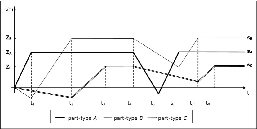
or 0. Figure 1 shows the evolution of the inventory level

of three part-types (A, B and C), taking into account the priority ordering

{

A B C

, ,

}

and without an initial inventory

(

s

_A

( )

0

=

s

_B

( )

0

=

s

_C

( )

0

=

0

)

. For

0

≤ <

t

₁, when

( )

1

A A

s

t

=

z

,

x

_A

( )

t

=

µ

and

x

_B

( )

t

=

x

_C

( )

t

=

0

; for

t

₁

≤ <

t

₂, when

s

_B

( )

t

₂

=

z

_B,

( )

A A

x

t

=

d

,

x

_B

( )

t

= −

µ

d

_A and

x

_C

( )

t

=

0

; for

t

₂

≤ <

t

₃, when

s

_C

( )

t

₃

=

z

_C,

( )

A A

(4)

( )

B B

x

t

=

d

and

x

_C

( )

t

=

d

_C. At instant

t

₄ the machine adopts a “down” state in

which it is not able to produce anything. In instant

t

5 the machine adopts an “up”

state and begins producing part-type A again with a production rate equal to

µ

.

Figure 1. “Evolution of the inventory level of three part-types”.

The optimal general solution of the problem is not known. However, Shu and Perkins (2001) establish simple closed-form expressions for the optimal hedging points and the corresponding cost, assuming that the prioritised hedging point policy is applied and a priority order of the part-types is given. For part-type 1

* 1 1 1

1

z

γ

λ

−

=

and

2

* 1

1 1 2

1

J

c

γ

λ

−

= ⋅

and for part-type

j

>

1

1 *

1

_j

1

_j

j

j j

z

γ

λ

− −

−

=

−

and *

( )

* 2

j j j j

J

=

C

−

c

z

where 1 j j k k

D

d

=

∑

, u d

j j j

q

D

λ

µ

=

−

,

(

)

(

u

)

d

(

u

)

j

j d u

q

D

q

µ

γ

µ

−

+

=

−

+

,

(

)

(

)

1

* 1 1

1

2

1

j j j j j

j j j j

C

c z

γ

λ

γ γ λ

− − −



−



=



−



−









and the total cost is * *

1 n j j

J

=

∑

.

part-type A part-type B part-type C

t1 t2 t3 t4 t5 t6 t7 t8

(5)

Nevertheless, only initial results of the optimal priority ordering, summarised here in Section 3.1, are presented in Shu and Perkins (2001) and its authors point out that this is an area for future research.

This problem raises at least three questions: (i) What structure do optimal policies have? (ii) Given a priority ordering, how can the optimal values of the hedging points be calculated for hedging point policies? (iii) How can optimal orderings be found for prioritised policies?

As for many inventory management problems (Sethi & Thompson, 2000), it is very natural to approach the first two questions with the help of control theory. However, the third question corresponds to a family of scheduling problems in which the elements are characterised by the distribution of the times the machine spends in the “up” and “down” states and the cost function. The first objective of this note is to place the problem in the field of scheduling and relate it to other similar scheduling problems.

The distinction between disjunctive scheduling (a resource can execute one activity at a time at most) and cumulative scheduling (some resources can execute several activities in parallel, in our case several part-types, provided that their capacity is not exceeded) is well known. When a cumulative resource intervenes, elastic scheduling, i.e., the possibility of varying the amount of the resource assigned to any activity over time (Baptiste et al., 1999, 2001) may sometimes be applied. Therefore, the problems of the abovementioned family belong to the class of elastic, cumulative scheduling problems, which have mainly been dealt with in the field of project scheduling.

(6)

operational time in a state, before switching to the other. As is pointed out in Perkins (2004) the failure-prone problems are similar (or “dual”) to the problems in which a variable demand stream is assumed (Perkins & Sikrant, 2001; Tan, 2001). Obviously, they are also similar to some problems of production systems with random yields (see, for instance, Ben-Zvi & Grosfeld-Nir, 2007).

The rest of this note is organised as follows: Section 2 defines a lower bound for the problem. Section 3 and Section 4 introduce a test bed and present a computational experiment in which the test bed is used to explain three dynamic programming approaches for determining optimal priority orderings. This test bed, the lower bound defined, the procedures developed and the optimal priority orderings obtained for the instances of the test bed will allow evaluating the performance of future heuristic and metaheuristic procedures. Section 5 outlines brief conclusions.

2 Calculating a lower bound

In Sánchez (2007) it is proved that the sign of the first derivative of the expected sum of quadratic holding and storage costs corresponding to a part-type

j

,

J

*j,

according to

D

_j₋₁,

*

1

j

dJ

dD₋ , is always positive (see an sketch of the proof in the

Annex). Therefore, function *

j

J

is strictly increasing according to

D

_j₋₁. This means

that the real quadratic holding and storage costs of a part-type

j

in the

i

th

position of the priority ordering is not less than the cost of this product assuming that the

( )

i

−

1

preceding products are those of minor demand rates (excluding

j

).

Therefore, a lower bound for the problem can be calculated as follows: We obtain

the quadratic holding and shortage inventory cost to sequence each part-type

j

(

j

=

1,...,

n

)

in the

i

th position of the priority ordering

(

i

=

1,...,

n

)

, taking into

account that the

( )

i

−

1

preceding products are those of minor demand rates

(excluding

j

). Then, a square matrix of costs

Q

of dimension

n

is obtained. The

lower bound is calculated by resolving the assignment problem with

Q

. In this

note we use the Jonker and Volgenant algorithm (Jonker & Volgenant, 1987),

(7)

3 Determining the optimal priority orderings

3.1 Introduction

Shu and Perkins (2001) show that the expected cost corresponding to a part-type does not depend on the order of the part-types with greater priority, but only on the sum of all their demand rates. They also show that placing

i

directly before

j

when a part-type

i

dominates a part-type

j

yields a cost that is no greater than

the cost corresponding to placing

j

directly before

i

(i.e., in order to find an optimal priority ordering there is no need to take into account orderings in which

j

is placed immediately before

i

). The definition of the dominance relations that we

use in the present note is as follows,

i

dominates

j

if and only if one of the three

following conditions is fulfilled: (i)

c

i

>

c

j and

c d

i

·

i

≥

c d

j

·

j; (ii)

c

i

=

c

j and

·

i i j j

c d

>

c d

; or (iii)

c

_i

=

c

_j,

d

_i

=

d

_j and

i

<

j

(we have added this last condition in

order to avoid reciprocity in the dominance relation).

These two properties allow the enumerative effort involved in finding an optimal priority ordering to be reduced. If there are no domination relations between pairs of part-types, or if these relations are not used, the computational complexity of

the calculations is proportional to 1

1

·

·2

1

n

n k

n

k

− =

−





=



−







∑

. Of course, the domination

relations, insofar as they reduce the number of orderings that need to be taken into account, help to reduce the computational effort.

3.2 Three dynamic programming approaches

The first property exposed in the previous subsection leads to approach the optimisation problem with dynamic programming. We have adopted the following decisions in our implementation of a dynamic programming scheme:

• The solutions are coded employing a vector

{

p p

₁

,

₂

,...,

p

_n

}

, where

p

_j

denotes the part-type sequenced in the

j

th position of the priority

ordering. A state

q

in the

k

th stage of the dynamic programming

procedure is defined by the set of the

k

already prioritised part-types

(8)

depend on the order of the part-types with greater priority, but only on the sum of all their demand rates). This is represented by a partial sequence in which prioritised part-types are ordered from lowest to highest according to their product index. If dominance relations are used, the characterisation of a state must also include an indication of which element is the last in the set,

p

k. In order to increase the efficiency of the procedure, a bijective

correspondence between the code of each state

q

of the

k

th stage and its

position in the table that contains the states of the

k

th stage has been

established.

• In each state

q

of the

k

th stage, the next part-type in the priority

ordering,

p

k+1, needs to be determined. This part-type must not yet be

prioritised and, if the dominance relations defined in Section 3.1 are used, this part-type should not be dominated by the last part-type in the partial preceding priority ordering.

• Let

Γ

k be the set of states belonging to the

k

th stage (where

{ } { }

{

}

1

1 ,...,

Γ =

n

)

;

χ

*_{k q}_, and

χ

*_k₋_1,_s, respectively, the optimal costs

corresponding to the state

q

of

k

th stage, and to the state

s

of

k

−

1

th

stage; and ₍* ₎

1, ,

κ

₋ k

k s p , the cost of adding

p

k as the

k

th part-type in the

partial priority ordering that defines the state

s

of

k

−

1

th stage.

The recursive function is as follows:

( )

(

)

1

* * *

,

min

_s 1, 1, ,

;

2,...,

χ

κ

− − −

∀ ∈Γ

=

+

∀ ∈Γ

=

k k

k q k s k s p

q

k

n

The costs ₍* ₎

(

)

1, ,

2,...,

κ

₋

=

k

k s p

k

n

are computed as indicated for the

*

j

J

in

Section 1

(9)

Of course, the limitations of these procedures stem from the fact that the number of states increases exponentially as

n

increases. It is straightforward that for

n

>

1

part-types the maximum number of states is reached at stage

1

2

n

k

= 



+









(and

also, when

1

2

n

+

is an integer, at

1

2

n

k

=





+





−





); for instance, the number of

states for

n

=

23

at stages 11 and 12 is equal to 1,352,078. Finally, we also

designed a third dynamic programming approach that uses the lower bound defined in Section 2 but not the dominance relations introduced in Section 3.1. We

will denominate this procedure

DP

−

LB

. The introduction of bounds in the

dynamic programming scheme allows reducing the number of states considered in the search process. The operation is as follows:

• First, a feasible solution

X

(and the value of the objective function

Z

) is

calculated with a heuristic procedure. The heuristic used in this note consisted in determining the ordering of the part-types according to the non-increasing values of the product

d

j⋅

c

j (which is the best heuristic

developed in Sánchez, 2007).

• A lower bound is calculated in each state

q

from each

k

th stage. If the

lower bound value is lower than

Z

, the next part-type in the priority

ordering,

p

k+1, is determined. If it is not lower than

Z

, the state

q

is

rejected.

• If the dynamic programming does not provide a solution,

X

is an optimal

solution.

As shown in Section 4, procedure

DP

−

LB

yields the worst results. Thus, we

decided not to define a dynamic programming approach that used jointly the lower bound and the dominance relations.

(10)

4 Computational experiment

First, we introduce a test bed for the problem. Then we report the results of a computational experiment in which optimal priority orderings for the instances of the test bed were determined using the three dynamic programming approaches defined in Section 3.2.

4.1 A test bed for the problem

To the authors’ knowledge, there is no standard test bed for the problem. Therefore, the following test bed was generated: the set consisted of 1,400 instances, 100 instances for each value of

n

in

[10, 23]

; the values of

d

j and

c

j

were generated at random using uniform discrete distributions in

[1,100]

and

[1, 20]

respectively.

In order to guarantee that the machine had enough capacity to meet demand, the

value of

µ

was set equal to

1

n d u

j j u

q

d

q

α

=

+

⋅

∑

, where

α

>

1

. Given the statement of

the problem, the influence of the values of

α

and the ratio d u

u

q

+

on the

computing times was assumed to be insignificant. This assumption was confirmed by performing a short, initial experiment using 25 instances in which

n

=

18

with

the values

α

=

1.05,1.10,1.25,1.50, 2.00

and d u

3.00, 2.00,1.50,1.20,1.10

u

q

+

=

. For

the different combinations of the parameter values, the computing times for solving each instance turned out to be almost identical. Therefore, the parameter

values

α

and d u

u

q

+

could be fixed (specifically, we established that

α

=

1.10

and

1.20

d u

u

q

+

=

, and therefore that

1

1.32

n j j

d

µ

=

⋅

∑

).

Presenting the design of the test bed for this new scheduling problem was another purpose of the present technical note. It can be obtained from

(11)

4.2 Results of a computational experiment

The following three dynamic programming approaches were used in the computational experiment: an approach that only takes dominance relations

(

DP Yes

−

_

DR

)

into account, one that does not

(

DP

−

No DR

_

)

, and one that

takes into account the lower bound but not the dominance relations

(

DP

−

LB

)

.

These three procedures have different degrees of calculation difficulty and different numbers of generated states; hence, it was not possible to determine a priori which would be the most efficient.

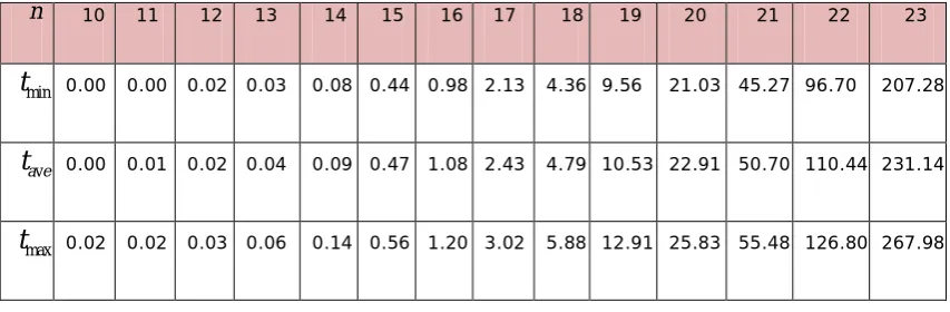
These three approaches were applied to the set of instances generated in subsection 4.1. The experiment was performed on a PC Pentium IV, at 3.2 GHz, with 1 Gb RAM. Table 1 shows the minimum

( )

t

min , average

( )

t

a ev and maximum

( )

t

max computing times in seconds, which correspond to applying

DP

−

No DR

_

.

n 10 11 12 13 14 15 16 17 18 19 20 21 22 23

min

t

0.00 0.00 0.02 0.03 0.08 0.44 0.98 2.13 4.36 9.56 21.03 45.27 96.70 207.28

v

a e

t

0.00 0.01 0.02 0.04 0.09 0.47 1.08 2.43 4.79 10.53 22.91 50.70 110.44 231.14

max

t

0.02 0.02 0.03 0.06 0.14 0.56 1.20 3.02 5.88 12.91 25.83 55.48 126.80 267.98

Table 1. “Minimum, average and maximum computing times (in seconds) with

_

DP−No DR”.

One can appreciate the low dispersion of the computing times for a given value of

n

, and furthermore that the ratio between the average computing times

corresponding to

n

and

n

−

1

is approximately equal to

2·

1

n

−

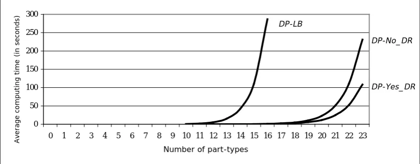
, as could be

expected from the analysis of the complexity of the algorithm. Figure 2 shows the average computing time as a function of the number of part-types,

n

.

The computing times using

DP Yes

−

_

DR

depend on the density of these

(12)

equal to

n n

·(

−

1) / 2

). Table 2 shows the minimum

(

%

min

)

, average

(

%

a ev

)

and

maximum

(

%

max

)

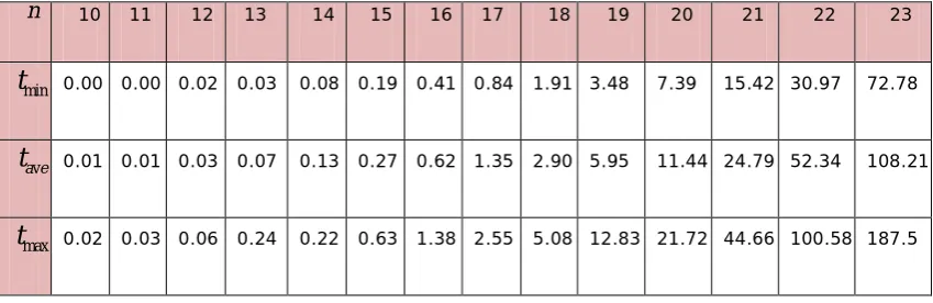
density of dominance relations corresponding to the set of

instances used in the experiment, expressed as percentages. Table 3 shows the minimum

( )

t

min , average

( )

t

a ev and maximum

( )

t

max computing times in seconds

using

DP Yes

−

_

DR

.

n 10 11 12 13 14 15 16 17 18 19 20 21 22 23

min

%

35.6 47.3 48.5 57.7 56.0 56.2 50.0 54.4 57.5 59.1 59.5 58.1 61.0 50.2

v

%

_{a e} 76.2 76.0 78.4 75.8 75.6 77.8 77.2 76.5 75.5 75.9 76.7 77.6 75.9 75.5

max

%

97.8 98.2 97.0 92.3 93.4 95.2 94.2 91.2 88.9 90.6 88.4 94.8 87.0 88.9

Table 2. “Minimum, average and maximum density of dominance relations (in %)”.

n 10 11 12 13 14 15 16 17 18 19 20 21 22 23

min

t

0.00 0.00 0.02 0.03 0.08 0.19 0.41 0.84 1.91 3.48 7.39 15.42 30.97 72.78

v

a e

t

0.01 0.01 0.03 0.07 0.13 0.27 0.62 1.35 2.90 5.95 11.44 24.79 52.34 108.21

max

t

0.02 0.03 0.06 0.24 0.22 0.63 1.38 2.55 5.08 12.83 21.72 44.66 100.58 187.5

Table 3. “Minimum, average and maximum computing times (in seconds) with

_

DP Yes− DR”.

In general, the computing times are shorter when dominance relations are used

than when they are not used. However, the dispersion for a given value of

n

is

greater, as was expected. The average computing times increase exponentially with the value of

n

, as occurs when dominances are not taken into account (Figure

(13)

0 50 100 150 200 250 300

0 1 2 3 4 5 6 7 8 9 10 11 12 13 14 15 16 17 18 19 20 21 22 23

Figure 2. “Average computing time versus number of part-types”.

Table 4 allows comparing, for

10

≤ ≤

n

16

the average computing times in seconds

that correspond to applying

DP

−

LB

and

DP

−

No DR

_

(

DP

−

LB

is similar to

_

DP

−

No DR

, but it uses the lower bound).

n 10 11 12 13 14 15 16

DP−LB 0.71 1.98 5.38 15.29 42.51 109.94 286.50

_

DP−No DR _0.00 _0.01 _0.02 _0.04 _0.09 _0.47 _1.08

Table 4. “Average computing times (in seconds) with DP−LB and DP−No DR_ ”.

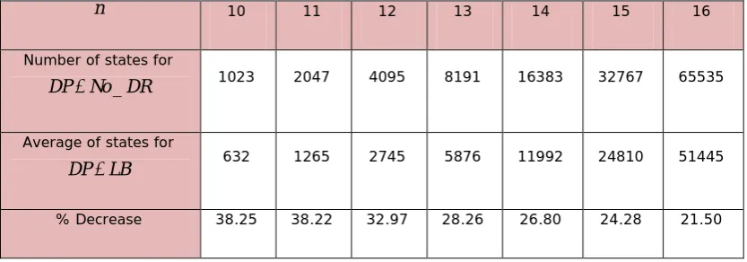
With the application of the lower bound, the computing times not only do not decrease but in fact they increase considerably (see also Figure 2). Using the lower bound in the dynamic programming procedure involves a decrease in the number of states compared to not using it, as can be seen in Table 5. The reason why the

computing times corresponding to

DP

−

LB

are higher than those corresponding to

_

DP

−

No DR

may be that, for

DP

−

LB

, the lower bound has to be calculated in

every state and this takes more time than when it is not calculated (when certain rejected states are not considered).

To sum up, the computational experiment shows that it is worthwhile using dominance relations and that instances with up to approximately 25 part-types can

be solved in relatively short computing times with the procedure

DP Yes

−

_

DR

.

DP-No_DR

DP-Yes_DR

Number of part-types

A

ve

ra

ge

co

m

pu

tin

g t

im

e

(i

n

se

con

(14)

The values of the optimal solutions of the instances of the test bed can be obtained

from

n 10 11 12 13 14 15 16

Number of states for _

DP−No DR 1023 2047 4095 8191 16383 32767 65535

Average of states for

DP−LB 632 1265 2745 5876 11992 24810 51445

% Decrease 38.25 38.22 32.97 28.26 26.80 24.28 21.50

Table 5. “Number of states with DP−No DR_ and average of states for DP−LB”.

5 Conclusions and research prospects

This work establishes optimal priority orderings for prioritised hedging point (PHP) control policies in the problem of minimising the expected sum of quadratic holding and shortage inventory costs when a single, failure-prone machine produces multiple part-types.

In this note, the problem is placed in the field of scheduling and a lower bound for the problem is proposed. Three dynamic programming approaches for determining optimal priority orderings are explained and a test bed is introduced. Finally, a computational experiment in which the algorithms are applied to the test bed is presented. This test bed, the lower bound proposed, the procedures developed and the optimal priority orderings obtained for the instances of the test bed allow the performance of future developments to be evaluated.

The computational experiment shows that it is worthwhile using dominance relations and that instances with up to approximately 25 part-types can be solved in relatively short computing times. Moreover, using the lower bound in a dynamic programming scheme increases the computing time needed. However, as the

memory required and the computing time increase exponentially with

n

, in order

to solve larger instances future research must be based on:

(15)

b) Using the lower bound only in some states of the multistage graph of

dynamic programming—for example, using the lower bound only in states with a high value of the partial solution built so far, which are more likely to be eliminated by taking into account the lower bound.

Annex

In this Annex it is proved that the sign of the first derivative of the expected sum of quadratic holding and storage costs corresponding to a part-type

j

,

J

*j, respect

to

D

j−1, *

1

j

dJ

dD₋ , is always positive. Maple © and Derive 5 © commercial software

have been used to help in this proof.

According to the terminology presented in Section 1

(

)

(

)

1

* 1 1

1

2

1

j j j j j

j j j j

C

c z

γ

λ

γ γ λ

− − −



−



=



−



−









, * 1

1

_j

1

_j

j

j j

z

γ

λ

− −

−

=

−

, u d

j j j

q

D

λ

µ

=

−

and

(

)

(

u

)

d

(

u

)

j

j d u

q

D

q

µ

γ

µ

−

+

=

−

+

), the expected sum of quadratic holding and storage costs

corresponding to a part-type

j

,

J

*j

=

C

j

−

c

j

( )

z

*j 2, can be expressed as follows (1):

* 3 2 2 2

1 1

(2

(

) (

)

(

) (2

(

) (

)

j j d u j j d u d u j d u j d u d u

J

=





c

⋅µ ⋅ ⋅ ⋅

q

d

⋅

D

₋

⋅

q

−

q

⋅

q

+

q

+

D

₋

⋅

q

+

q

⋅

d

⋅

q

+

q

⋅

q

−

q

2 2 3

1

(4

))

(2

(

)

(

2

)))] /[(

) (

(

)

u u d u j d u d u d u j d u u

q

d

q

D

q

µ

−

µ

+ ⋅ ⋅

−

+ ⋅ ⋅

⋅

+

− ⋅

+

⋅

+

− ⋅

2 1

(

D

_j₋

(

q

_d

q

_u

)

d

_j

(

q

_d

q

_u

)

µ

q

_u

) ]

⋅

+

⋅

+

− ⋅

(1)

Then, we calculate the first derivative of *

j

J

respect to

D

_j₋₁:

*

2 3 3 2 2

1 1

1

[2

(3

(

) (

)

(

) (5

(

) (

)

j

j j d u j d u d u j d u j d u d u

j

dJ

c d

q q

D

q

D

q

d

q

dD

−

µ

− −

= −

⋅ ⋅

⋅ ⋅ ⋅

⋅

−

⋅

+

⋅

+

⋅

+

⋅

−

2 2

1

3

µ

q

u

(3

q

u

q

d

))

D

j−

(2

d

j

(

q

d

q

u

) (

q

d

q

u

)

2

d

j

µ

q

u

(

q

d

q

u

) (5

q

u

q

d

)

+

⋅ ⋅

−

+

⋅

−

⋅

+

⋅ ⋅ ⋅

+

⋅

−

2 2 2 2 2

3

µ

q

u

(

q

d

3 ))

q

u

µ

q

u

(

d

j

(

q

d

q

u

) (

q

d

2

q

u

)

d

j

µ

q

u

(3

q

d

5 ) 3

q

u

µ

q

u

))] /

−

⋅ ⋅

+

+ ⋅ ⋅

⋅

+

⋅

+

− ⋅ ⋅ ⋅

+

⋅

3 4

1 1

(16)

Taking into account that

c

_j

>

0

,

d

_j

>

0

,

µ

>

0

,

q

_u

>

0

,

q

_d

>

0

,

1 j j k k

D

d

=

∑

, 4 1

(

D

j−

⋅

(

q

u

+

q

d

)

− ⋅

µ

q

u

)

>

0

and

3 1

(

D

j−

⋅

(

q

u

+

q

d

)

+

d

j

⋅

(

q

u

+

q

d

)

− ⋅

µ

q

u

)

<

0

(because

(

)

1

/(

)

n

u d u j

j

q

µ

q

d

=

⋅

+

>

∑

), the sign of (3) has to be studied (it must be positive for

the proof):

3 2 2

1 1

(3

D

_j₋

⋅

(

q

_d

−

q

_u

) (

⋅

q

_d

+

q

_u

)

+

D

_j₋

⋅

(

q

_d

+

q

_u

) (5

⋅

d

_j

⋅

(

q

_d

+

q

_u

) (

⋅

q

_d

−

q

_u

) 3

+

µ

⋅ ⋅

q

_u

(3

q

_u

−

q

_d

))

2 2 2 2

1

(2

(

) (

)

2

(

) (5

) 3

(

3 ))

j j d u d u j u d u u d u d u

D

₋

d

q

d

µ

q

µ

q

+

⋅

−

⋅

+

⋅ ⋅ ⋅

+

⋅

−

⋅ ⋅

+

2 2 2

(

) (

2

)

(3

5

) 3

))

u j d u d u j u d u u

q

d

q

d

q

µ

+ ⋅ ⋅

⋅

+

⋅

+

−

⋅ ⋅ ⋅

+

⋅

(3)

Given that the units used to express the demand rate may be chosen arbitrarily, one can take, without loss of generality,

d

_j

=

1

and replace

D

_j₋₁

/

d

_j with

X

. This

way, expression (3) is reduced to expression (4):

3 2 2

(3

X

⋅

(

q

_d

−

q

_u

) (

⋅

q

_d

+

q

_u

)

+

X

⋅

(

q

_d

+

q

_u

) (5 (

⋅ ⋅

q

_d

+

q

_u

) (

⋅

q

_d

−

q

_u

) 3

+

µ

⋅ ⋅

q

_u

(3

q

_u

−

q

_d

))

2 2 2

(2 (

_d _u

) (

_d _u

)

2

_u

(

_d _u

) (5

_u _d

) 3

_u

(

_d

3 ))

_u

X

q

µ

q

µ

q

+ ⋅ ⋅

−

⋅

+

⋅ ⋅

+

⋅

−

⋅ ⋅

+

2 2

((

) (

2

)

(3

5

) 3

))

u d u d u u d u u

q

µ

+ ⋅ ⋅

+

⋅

+

− ⋅ ⋅

+

⋅

(4)

Replacing

(

q

_u

+

q

_d

)

with

C

and

µ ⋅

q

_u with

B

, expression (4) is reduced to

expression (5):

3 2 2

3

X

⋅

(

C

−

2

q

_u

)

⋅

C

+

X

⋅ ⋅

C

(5

C C

⋅

(

−

2

q

_u

) 3

−

B C

⋅

(

−

4

q

_u

))

2 2

(3

(

2

_u

)

2

(

6

_u

) 2

( 2

_u

)

X

B

C

q

B C C

q

C

q

C

− ⋅

⋅

+

⋅ ⋅

−

− ⋅

⋅

2

(3

2

_u

)

(

_u

))

B

C

q

C C

q

+ ⋅

− ⋅

+

+ ⋅

+

(5)

The expression

(

q

_u

⋅

µ

) /(

q

_u

+

q

_d

)

>

D

_j₋₁

+

d

_j is equivalent to expression

B C

>

X

+

1

and

C

>

0

. Therefore

B

> ⋅

C

(

X

+

1)

and we can set

B

= ⋅ ⋅

A C

(

X

+

1)

, where

A

>

1

(see expression (6)):

3 3 3 2 3 3 2 2 3 3 3 2 3 3 3 2 3

3

A C

⋅

X

−

3

A C

⋅

X

−

6

A C

⋅

X

⋅ −

q

_u

3

A C

⋅

X

+

12

A C

⋅

X

⋅ +

q

_u

3

C

⋅

X

−

6

C

⋅

X

⋅

q

_u

3 3 2 2 3 2 2 2 2 3 2 2 2 3 2 2 2

9

A C

X

9

A C

X

14

A C

X

q

_u

5

A C

X

24

A C

X

q

_u

5

C

X

10

C

X

q

_u

+

⋅ ⋅

−

⋅ ⋅

−

⋅ ⋅

⋅ −

⋅ ⋅

+

⋅ ⋅

⋅ +

⋅

−

⋅

3 3 2 3 2 2 3 2 3 2

9

A C

X

9

A C

X

10

A C

X q

u

A C

X

13

A C

X q

u

2

C

X

4

C

X q

u

+

⋅

⋅ −

⋅

⋅ −

⋅

⋅ ⋅ − ⋅

⋅ +

⋅

⋅ ⋅ +

⋅ −

⋅ ⋅

3 3 2 3 2 2 3 2

3

A C

3

A C

2

A C

q

_u

A C

q

_u

(17)

The sign of the coefficients of 3

X

, 2

X

, 1

X

and 0

X

can be studied separately, in

order to show that they are always positive and that, therefore, taking into account that

X

≥

0

, the whole expression (2) is positive.

As an example, we prove that the sign of the coefficient of 3

X

is positive. Expression (7) shows, taken from (6) the expression that gives the value of this coefficient:

3 3 2 3 2 2 3 2 3 2

3

A C

⋅

−

3

A C

⋅

−

6

A C

⋅

⋅ −

q

_u

3

A C

⋅

+

12

A C

⋅

⋅ +

q

_u

3

C

−

6

C

⋅

q

_u (7)

Whose sign is the same than that (8):

3 2

2

4

2

(

3 2

1)

( 2

2

4

2)

u u u u

A C

⋅ −

A C

⋅ −

A

⋅

q

− ⋅ +

A C

A q

⋅

+ −

C

q

= ⋅

C

A

−

A

− + +

A

q

⋅ −

A

+

A

−

(8)

Remember that

A

>

1

. Then, the coefficient of

C

is positive

(

A

3

−

A

2

− + >

A

1 0)

.

However, the coefficient of

q

u is negative

2 2

( 2

−

A

+

4

A

− = − −

2

(

A

1) )

.

As

C

=

(

q

_u

+

q

_d

)

, to prove that 3 2 2

(

1)

u

( 2

4

2)

0

C

⋅

A

−

A

− + + ⋅ −

A

q

A

+

A

−

>

it suffices

to show that 3 2 2

(

1)

( 2

4

2)

0

C

⋅

A

−

A

− + + ⋅ −

A

C

A

+

A

−

>

, which is equivalent to show

that 3 2 2 3 2

(

A

−

A

− + + −

A

1)

( 2

A

+

4

A

−

2)

=

A

−

3

A

+

3

A

− >

1

0

. And this last

proposition is straightforward, since

A

>

1

and the expression is equal to 0 for

1

A

=

and its derivative

(

3

A

2

−

6

A

+

3

)

is > 0 for

A

>

1

.

References

Bai, S. X., & Gershwin S. B. (1994). Scheduling manufacturing systems with work-in-process inventory control: multiple-part-type systems. International Journal of

Production Research, 32, 365-385.

Baptiste, Ph., Le Pape, C., & Nuijten, W. (1999). Satisfiability tests and time_bound adjustments for cumulative scheduling problems. Annals of Operations Research, 92, 305-333.

Baptiste, Ph., Le Pape, C., & Nuijten, W. (2001). Constraint-based scheduling.

(18)

Ben-Zvi, T., & Grosfeld-Nir, A. (2007). Serial production systems with random yields and rigid demand: A heuristic. Operations Research Letters, 35, 235-244.

Corominas, A., & Pastor, R. (2009). Scheduling production of multiple part-types in a system with pre-known demands and deterministic inactive time intervals.

European Journal of Operational Research, 193, 639-643.

Hu, J. Q., & Xiang D. (1995). Optimal control for systems with deterministic production cycles. IEEE Transactions on Automatic Control, 40, 782-786.

Jonker, R., & Volgenant, A. (1987). A shortest augmenting path algorithm for dense and sparse linear assignment problems. Computing, 38, 325-340.

Ketzenberg, M., Metters, R., & Semple, J. (2006). A heuristic for multi-item production with seasonal demand. IIE Transactions, 38, 201-211.

Perkins, J. R. (2004). Optimal control of failure-prone manufacturing systems with constant repair-times. Annals of Operations Research, 125, 233-261.

Perkins, J. R., & Srikant, R. (1997). Scheduling multiple partt-types in an unreliable single machine manufacturing system. IEEE Transactions on Automatic Control, 42, 364-377.

Perkins J. R., & Srikant, R. (2001). Failure-prone production systems with uncertain demand. IEEE Transactions on Automatic Control, 46, 441-449.

Sánchez, A. (2007). Determinación de secuencias en una máquina multiproducto sujeta a fallos y con costes cuadráticos. Doctoral Thesis, Universitat Politècnica de Catalunya, Barcelona.

Shu, C., & Perkins, J. R. (2001). Optimal PHP production of multiple part-types on a failure-prone machine with quadratic buffer costs. IEEE Transactions on Automatic

Control, 46, 541-549.

Sethi S. P., & Thompson, G. L. (2000). Optimal control theory: Applications to

management science and Economics, 2nd edition. Kluwer.

(19)

Article's contents are provided on a Attribution-Non Commercial 3.0 Creative commons license. Readers are allowed to copy, distribute and communicate article's contents, provided the author's and Journal of Industrial Engineering and Management's names are included. It must not be used for commercial purposes. To see the complete

doi:10.3926/jiem.2009.v2n3.p418-436