Issues
ISSN: 2146-4138
available at http: www.econjournals.com
International Journal of Economics and Financial Issues, 2017, 7(6), 104-110.
Study About the Minimum Value at Risk of Stock Index Futures
Hedging Applying Exponentially Weighted Moving Average
- Generalized Autoregressive Conditional Heteroskedasticity
Model
Rong Xu
1*, Xingye Li
21University of Shanghai for Science and Technology, Shanghai, China, 2University of Shanghai for Science and Technology,
Shanghai, China. *Email: ronger52910@163.com
ABSTRACT
What investors often wish to insure is that the maximum possible loss of their portfolios falling below a certain value. Namely, the maximum possible loss that a portfolio will lose under normal market fluctuations, with a given confidence level, over a certain time horizon, it is known shortly as “value at risk (VaR).” However, when it comes to the hedging strategy taking in the derivative markets for the minimum VaR, many investors simply thinking it is a hedging ratio in one at beginning, then a lot of effective model came out from both academia and industry over the years.We pioneer deriving a combined and dynamic hedging model- exponentially weighted moving average-generalized autoregressive conditional heteroskedasticity (GARCH) (1,1)-M applicable to the real financial markets based on previous studies. The results in this paper turn out that the model we build is not only excellent for the pursuit for the minimum VaR but also practical for the actual situation where the variances of financial price data are time-varying.In this paper we calculate the optimal decay factor 0.93325 which is the best match to the Hu-Shen 300 stock index market, withdraw uniform 0.9400, and use the Cornish-Fisher function to correct the quantile of the normal distribution, get the final hedging ratios and the minimum VaR.
Keywords: Minimum Value At Risk, Hedging Model, Decay Factor, Cornish-Fisher, Exponentially Weighted Moving Average -Generalized Autoregressive Conditional Heteroskedasticity (1,1)-M Model
JEL Classifications: G11.
1. INTRODUCTION
Chinese futures market had developed rapidly as the importantly emerging derivatives market over the world since the beginning of the 1990s. Its first introduction of financial futures-Hu-Shen 300 stock index futures is in April 16, 2010.Their came out successfully opened a new era when investors can short in Chinese A-shares markets, ended the embarrassing status of unilateralism, which play an vital role in pushing the healthy development of the security market, established a milestone in the financial futures market. Due to the not long time running of the trading of stock index futures in Chinese financial market, there had no a mature trading mechanism yet in the market, always facing various trading risk, such as price risk, political risk, law risk, operation risk and credit risk which was intensified by the unique characteristic –“margin
trading” in futures market. In order to restore the distorted markets function in price discovery, curb excessive speculation, increase the market liquidity, reduce investor’s risk, improve the return of portfolios, then hedging strategies has gained much more focus, and the research programs about hedging strategy are not uncommon both in China and abroad.
Hu-Shen 300 stock index futures take the Hu-Shen 300 stock index as its underlying assets, its ability of hedging can averse the systematic risk in securities market, and help investors to control risk in themselves investment products. The detrusion of Hu-Shen 300 stock index futures providing a favorable investment environment to investors.
position by holding opposite futures contracts in futures market, covering their loss in one market by using another gain and realizing their aim of risk aversion in market. The core problem in hedging strategy is constructing a portfolio to decide the hedging ratio, traditional theory simply believed that the ratio is 1, means that we can hedging 1 spot to avoid the price risk with 1 future, which is based on the ideal condition that the price changed in spots market are in the same pace with the future contractions, but owe to many irrational and unexpected speculator, and the leverage effect because of margin trade, all these increasing the risk of price fluctuation to a greater extent, making the price changed are not in the same pace completely between futures and spots, then we need to build a appropriate hedging model according to the price volatility of spots and futures in every market day, and estimate the optimal hedging ratio, then analyze the performance of hedging strategy.
At present, as the common state of volatility clustering and leptokurtosis and heavy tails in the financial data, majority of the hedging strategies are built under the guidance of the generalized autoregressive conditional heteroskedasticity (GARCH) model, which developed by Bollerslev based on the ARCH model introduced by Engel.
As far as the research of Chinese stock index futures market, most of them use the existing foreign documents for reference. some of them use foreign financial data or the mock trading data from the Hu-Shen 300 stock index futures market for empirical studies. In the paper of Chongfeng et al. (1998), they completed their empirical analysis of the hedging strategy by using numerical calculation method of the optimal hedging ratio, and analyzed their correlation and effectiveness aimed at the minimum risk and maximum utility according to the real copper data from Shanghai metal exchange. Then Hui and Jinwen (2007) introduced the co-integration in their research of the better hedging performance of Hu-Shen 300 stock index. We know that previous exponentially weighted moving average (EWMA) model used to estimate the hedging ratio of Hu-Shen 300 stock index futures are unity using the decay factor in 0.9400.
To the best of our knowledge, this paper take some references for previous research to rebuild the optimal hedging model. In fact, in consideration of the characteristic of risk premium of the return in financial market, and the feasibility and performance of the GARCH(1,1)-M model, we build the EWMA-GARCH(1,1)-M model to calculate the optimal decay factor, then we use the Cornish-Fisher formula to amend the fractile quantiles of normal distribution, get the revised fractile quantiles of return series, and we eliminate the negative quantiles reasonably, get the optimal hedging ratio.
Furthermore, the value at risk (VaR) we estimate remarkably less than those estimated by traditional models, which turn out that our model is in the excellent performance of hedging. We work out that the VaR of such portfolio submit to the normal distribution in some degree, and our model can effectively predict the future VaR, and direct the hedging traders, confine the portfolio risk. We hereby declare that the significance level in the process paper’s
writing and data examination using the uniform default α = 0.05 for the accuracy of data analysis.
The remainder of this paper proceeds as follows, section 2 presents our modified theoretical hedging model applicable to the Hu-Shen 300 stock index futures market. In section 3, we exam this model by using the real data from Hu-Shen 300 stock index futures market. The results proves that such a hedging model is effective and in better performance than many other old models.
2. MODEL SETUP
2.1. VaRHere in order to be consistent with the daily habits, the VaR takes a positive form.
Let rs and rf denote the logarithmic return rate of spots and futures respectively, and h denotes the hedging ratio (namely that per unit spot needs h unit futures to hedge), then the return rate of portfolio rp presents as below:
rp = rs-hrf (1)
According to the definition (Jorion, the VaR in the percentage of (1-α) of the above financial asset portfolio can be expressed as following:
VaRp (1-α) = µp+σpqp (α) (2)
Where the µp = E (rp) denotes the expected return rate of the portfolio, σp = var(rp)(1/2) denotes the standard deviation of the
return rate of the portfolio. We assumed that µp = 0, and qp (α) is the lower quantile in the standardized distribution of the return rate of the portfolio.
A large number of empirical studies have proved that the distribution of securities return, especially derivative return, does not comply with the normal distribution, but with the characteristics of obvious skewness, kurtosis, leptokurtosis and heavy tails. Therefore, it is not very reasonable here assumed that the return rate of the portfolio obey the normal distribution, and we amend the abnormal distribution with some effective measures.
Here we use the Cornish-Fisher formula to modify the quantile, which can be approximated by the skewness and kurtosis of the portfolio return rate, shown as following:
q n n S n n K
n n
p p p
^ ( )
(
α α α α α
α
=
( )
+(
( )
−)
+(
( )
−( )
)
−( )
−1
6 1
1
24 3
1
36 2 5
2 3
3
αα
( )
)Sp2 (3)S E r
E r hE r r h E r r h E r
h
p p
p
s s f s f f
s = =
( )
−( )
+( )
− + ( ) ( ) ( 3 33 2 2 2 3 3
2 2
3 3
σ σ σσf h r rs f
2−2 cov( , ))3 2/ (4)
K E r
E r hE r r h E r r h E r r h
p p
p
s s f s f s f
= ( )=
( )
−( )
+( )
−( )
+4
4
4 4 3 6 2 2 2 4 3 3 4
σ
E E r
h h r r
f
s f s f
( )
( cov( , ))
4
2 2 2 2 2
σ + σ −
(5)
We can infer the VaR based on the Cornish-Fisher formula from (3) and (2) as following:
VaRp
(
1−α)
= −σpq^p( )α = −(σs2+h2σf2−2hσsf)1 2/ q^p( )α (6)In order to minimize the VaR of a certain confidence region, the partial differential of VaR to hedging ratio h must satisfies the following condition: ∂ ∂ =
( )
+ × − + − VaR hh E r n
h
h h
f f sf
s f sf
( )
( )α σ σ
σ σ σ
2
2 2 2 2
(7)
We can get such a formula inferred from the first-order derivative:
E r n h
h h
f
f sf
s f sf
( )
+( )
× −+ − =
α σ σ
σ σ σ
2
2 2 2
2
0 (8)
The optimal hedging ratio in the confidence level of 1-α as following:
h h E r
E r n
sf
f f
f
sf f s
f f
= = − × −
−
2 2 2
2 2 2
2 2 2
σ σ σ
σ σ σ α σ
( )
( ( )) ( ( )) (9)
However, the return rate of the portfolio does not submit to the normal distribution, so the above formula calculated hedging ratio is not very accurate, through the formula (4), (5) can calculate the skewness and kurtosis of the portfolio, and then using the Cornish-Fisher formula to amend the quantile n(α), obtain the modified quantile, that is q^p( )α , the modified hedging ratio h2 is calculated by (9), and the VaR is calculated by using the formula (6), the VaR in this way satisfies the minimization condition.
According to the above analysis, we can see that the hedging ratio of the minimum VaR estimated by using Cornish-Fisher expansion formula need to calculate the futures and spots statistical magnitudes, if using the historical simulation method, requires mass of data, but Chinese Shanghai and Shenzhen 300 stock index futures is in a relatively short time-to-market, the amount of data is relatively small, the calculation accuracy is difficult to guarantee.
Cao et al. have demonstrated that the Cornish-Fisher expansion method is superior to the historical simulation method in terms of the hedging effect in the data of Out-of-Sample. However, the simple sample moment method cannot effectively capture the characteristics of volatility clustering and leptokurtosis and heavy tails of the financial data, and conclusions of many literatures about the minimum variance hedging strategy shows that the EWMA or GARCH model can improve the hedging effect. On the basis of Cao et al., the volatility modeling, conditional correlation model and Cornish-Fisher expansion method are combined to study whether our model can perform better when hedging.
2.2. EWMA-GARCH(1,1)-M
2.2.1. Estimation of variance based on the EWMA model
We denotes by {rt} the time series of return rate of the financial asset. Under the hypothesis of random walking {rt}, obey the independent normal distribution:
rt ∼N( ,µ σt2)
We assume that µ = 0 when studying the daily return rate.
2.2.2. EWMA
The EWMA model is revised from the traditional SAM, it can be expressed as following:
σ^ λ λ
( ) t i i t i r = − = ∞ −
∑
1 0 2 (10)This method is characterized by the fact that each observed date of return rate is given a different weight, the closer the return rate from the current observation time, the greater of the weight of the return rate, and the further is reverse. The λ(0<λ<1) in (10) named decay factor. Its size determines the weight of the relevant samples and the length of the effective samples, its value in the domain of 0~1.
We denotes by t2+1t
/ the return rate before time t (including time t) explicitly, and estimate the variance of the return rate at time t+1, inferring from (10) as following derivation:
σt2+1/t =λσ^t t2/−1+ −(1 λ)rt2 (11) However, the calculation of the previous decay factor usually uses the grid method to calculate the minimum mean square error of each risk factor and the corresponding value of λ, and then calculate the weight of each λ, and finally weighted to the optimal daily decay factor in Chinese financial market, which is approximately λ = 0.9400.
2.3. EWMA-GARCH(1,1)-M
2.3.1. Principle of EWMA- GARCH(1,1)-M
We operate data analysis of the Hu-Shen 300 stock index futures find that the GARCH(1,1) -M model can be established and applicable for spots and futures return rate, and the lag coefficient of the variance equation of the model can be estimated, then combining the EWMA for a comprehensive estimation of the decay factor. This estimation takes into account the characteristics of volatility clustering and risk premium of the return rate, and the comprehension of a variety of factors, making the decay factor be in higher accuracy.
2.3.2. Setup of EWMA-GARCH(1,1)-M
The formulation of GARCH(1,1)-M can expressed as following:
σ λσ λ
µ σ
σ ε
t t t t t
t t t
t t t
r
r c a
a + = − + − = + + = 1 2 1 2 2 1 / ^ / ( ) (12)
σ λσ λ
σ α α β σ
t t t t t
t t t t t
r a + − + − = + − = + + 1 2 1 2 2 1 2
0 1 2 1 2 1
1 / ^ / / / ( ) (13)
It is not difficult to find similarities between the above-mentioned two formulas. The lag coefficient β in the GARCH model mainly reflects the correlation of the volatility of prediction data and historical data, while the λ in the EWMA model also reflects the correlation of the volatility of prediction data and historical data, there does appear to be a link between these two formulas. For the assumption that GARCH(1,1) -M model is a stationary process, there is α1+β1≤1, let the decay factor in the EWMA model λ = max(β1, 1-α1), then estimate the lag coefficient of the conditional variance equation, all these are the process of building the EWMA-GARCH(1,1) -M model.
3. EMPIRICAL ANALYSIS
3.1. Data and IllustrationThe closing price of Hu-Shen 300 stock index and stock index futures of China Financial futures exchange is selected from the WIND database, here in all 431 observed data which from July 12, 2013 to April 20, 2015. We denote by pts the closing price of
Hu-Shen 300 stock index and by pft the closing price of its futures in day t, then the daily logarithmic return rate of them shown as following:
r = lnp lnp
r lnp lnp
t s t s t s t f t f t f − = − − − 1 1 (14)
3.2. Basic Statistical Analysis
Firstly, Eviews software is used to analyze the trend and the correlation coefficient of the price series of Hu-Shen 300 stock index and stock index futures. The correlation coefficients are shown in Table 1.
It can be seen from the Table 1 that there is a correlation coefficient as high as 0.9995 between the IF300 and CSI300.
Operating the ADF test to the logarithmic price series and return rate series of IF300 and CSI300 respectively, to exam whether they are stationary data, the test results shown in Table 2.
As we can see from the ADF test of the unit root in Table 2, we know that the logarithmic price series of IF300 and CSI300 are non-stationary, but the return rate series is stationary. Therefore, the next modeling process of the return rate series can be operated.
3.3. Setup of the GARCH(1,1)-M and Decision of the Optimal Decay Factor
Building regression equation (15) about rtf and rts based on OLS,
and operating ARCH test for (15), turn out that both rtf and rts
have ARCH effects, so we initially establish the GARCH model, and then in view of the fact that the financial return rate data have the characteristic of risk premium, then the GARCH(1,1) -M model of rtf and rts can be established.
Combining above equations, the GARCH(1,1)-M model about rts shown as follow:
rts = −0 001202 0 190128. + . Ã +µts ts (15)
Ãts2 =2 29. E−06 0 056683+ . µ2( )t−1s+0 931170. ( )2t−1s (16) Then combining (11), get following equations:
α0 = 2.29E-06, α1 = 0.056683, β1 = 0.931170, α1+β1≤1,
λ = max(β1, 1-α1), λ = 1-α = 1-0.056683 = 0.943317,
That is λ1 = 0.943317
Similarly, the GARCH(1,1)-M model about rtf shown as following:
E = −0.001210+0.183117σtf+εtf (17)
à =tf2 3 10. E−06 0 076817+ . µ( )2t−1f +0 910403. ( )2t−1f (18)
α0 = 3.10E-06, α1 = 0.076817, β1 = 0.910403, λ2 = 0.923183
Then get the optimal decay factor applicable for Hu-Shen 300 stock index and its futures markets, which is λ = (λ1+ λ2)/2 = 0.93325.
3.4. Computation of Optimal Hedging Ratio
3.4.1. Variance estimation based on EWMA
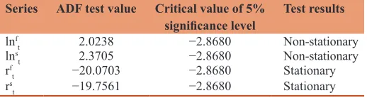
We calculate the optimal decay factor as λ = 0.93325, so we can use R statistical software to establish the EWMA model to compute the time-varying variance and covariance of rtf and rts, the graphs as shown in Figure 1.
3.4.2. Revised hedging ratio by Cornish-Fisher
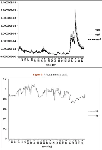
Put the time-varying variance and covariance data into (9), the hedging ratios of 430 trading days can be gotten, denote by h2 the hedging ratios, these are hedging ratios before operating Cornish-Fisher revision, put h2 into those equations in preceding text which calculate the skewness (Sp) and kurtosis (Kp) of portfolio, then put S and K into the formula (3) which revise the quantile of portfolio
Table 1: Correlation coefficients of the IF300 and CSI300
daily closing price
Correlation coefficient CSI300 IF300
CSI300 1.0000 0.9995
IF300 0.9995 1.0000
Table 2: Results of the ADF test of IF300 and CSI300 Series ADF test value Critical value of 5%
significance level Test results
lnf
t 2.0238 −2.8680 Non-stationary
lns
t 2.3705 −2.8680 Non-stationary
rf
t −20.0703 −2.8680 Stationary
rs
through Cornish-Fisher formula, get the modified quantile (q^p( )α ) of portfolio, and then put them into the formula (9), calculate the revised hedging ratio h3. The hedging ratios h2 (before amendment) and the hedging ratios h3 (after amendment) shown in Figure 2.
As is shown in the Figure 2, the hedging ratios before Cornish-Fisher amendment roughly matched the hedging ratios before the amendment, but in some certain period, the hedging ratios after the amendment is in higher fluctuation, turn out that the modified model can be more accurate and timely response to price fluctuations, so as to achieve the purpose of avoiding risk.
3.5. Estimation of the Minimum VaR
3.5.1. VaR based on EWMA-GARCH(1,1)-M
Put the revised hedging ratios h3 into (4), we can estimate the daily VaR within a given confidence level, denote by VaR1 the VaR. There appear a little positive value in VaR1 data, and this does not conform to the meaning of VaR, the reason of such a phenomenon is that some of the revised quantile of return rate of portfolio is negative, the hedging ratio calculated is fairly large in value, the number of futures for hedging completely offset even surpass the losses caused by the high volatility of spots price, all of these resulting in positive value in VaR1. For this case, in order to get more accurate estimation model of the hedging ratio, remove the
Figure 1: Time-varying variance and covariance based on exponentially weighted moving average
hedging ratio h3 which is in abnormal state, finally retain 304 valid data, also are 304 negative and effective VaRs, set VaR=VaR2. According to the statistical characteristics of VaR2, such data approximately obey the normal distribution, so this model can predict future VaR to control investment risk. Figure 3 shows the revised VaR2.
3.6. Comparisons with Traditional Hedging Model The traditional hedging theories hold that the futures and spot prices have exactly the same volatility, so the hedging ratio h = 1, and the formula to estimate the VaR of the portfolio shown as following:
VaR3=zα* *σ ∆t (19)
Denotes by zα the quantile in 0.95 (confidence level) of normal distribution, and α = 1.6449, denotes by σ the standard deviation
of return rate of the portfolio; Δt the holding period, then
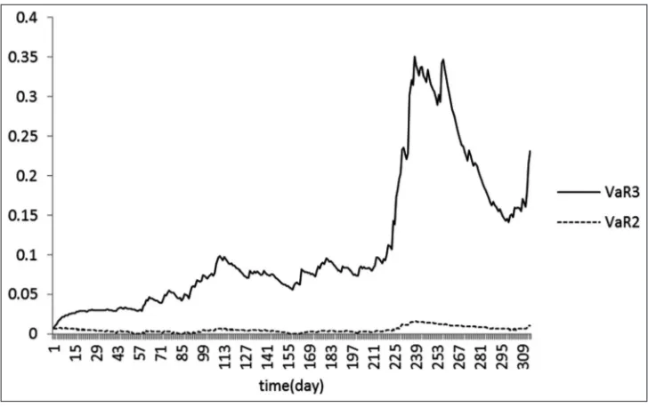
σ=(σs2+σf2−2cov ( , ))r rs f 1 2/ , we have estimated σ σ2s, f2, cov( , )r rs f through the EWMA, we can compare the VaR3 (traditional model) with the VaR2, shown as Figure 4.
The daily VaR processed by the EWMA-GARCH(1,1) -M model is much smaller than that of the traditional hedging model, indicating that the hedging effect of this model is excellent.
3.7. Analysis of the Effect of EWMA-GARCH(1,1)-M
To sum up, the VaRs of EWMA-GARCH(1,1)-M are lower than that of the traditional hedging model in the normal state, calculate the degree of VaR lowering, denotes V = (VaR3-VaR2)/VaR3, get the percentage of reduction each trading day, average the value, get V’ = 0.327879. All of these turn out that the EWMA-GARCH(1,1)-M model has good effect in risk-aversion.
Figure 3: Revised value at risk (VaR2)
Source: VaR here expressed in its absolute value
4. CONCLUSION
This paper combine the EWMA model with the GARCH(1,1)-M model to the EWMA-GARCH(1,1)-M model, then estimate the decay factor, to avoid the weakness of using constant decay factor to predict future time-varying variance, and for the characteristics of the volatility clustering and actual distribution of financial data, revise the quantile of the return rate of the portfolio through Cornish-Fisher method, we accurately calculate the hedging ratio. At the same time, remove the positive value of VaR data, which is in the purpose of reasonable theoretical research, then calculate the optimal hedging ratio, get the minimum VaR. Compared with the traditional model which has a simple hedging ratio in 1 and many other hedging strategies, our model is excellent for reducing the VaR of the portfolio. The EWMA-GARCH(1,1)-M model provides hedging investors with nice guidance.
REFERENCES
1. Chongfeng, W., Hongwei, Q., Wenfeng, W. (2008), Theoretical and empirical study about futures hedging [J]. Systems Engineering Theory Methodology-Applications, 7(4), 20-26.
2. Hui, G., Jinwen, Z. (2007), Empirical research for hedge ratio and shares portfolios of shanghai-shenzhen 300 shares index futures. Journal of Management Sciences, 20(2), 80-90.
3. Richard, T.B., Robert, J.M. (1991), Bivariate GARCH estimation of the optimal commodity futures hedge. Journal of Applied Econometric, 6(2), 109-124.
4. Cao, Z., Harris, Z.D.F., Shen, J. (2010), Hedging and value at risk: A semi-parametric approach. Journal of Futures Markets, 30(8), 780-794.
5. Hill, G.W., David, A.W. (1968), Generalized asymptotic expansions of cornish-fisher type. Annals of Mathematical Statistics, 39(4), 1264-1273.
6. Jorion, P., Philippe, B.J. (2000), Value-at-Risk: The New Benchmark for Controlling Market Risk. Irvine: University of California. 7. Jason, L., John, T. (2005), Hedging effectiveness of stock index
futures. European Journal of Operation Research, 163(1), 177-191. 8. Karanasos, M. (2001), Prediction in ARMA model with GARCH
in mean effects. Journal of Harts for in the Presence of Shifts in [J], Sequantial Analysis, 20(1-2), 1-13
9. Manuel, C.M., Yarema, O., Antonio, P., Wolfgang, S. (2001), Some stochastic properties of upper one-side and EWMA charts for in the presence of shifts. Sequantial Analysis, 20(1-2), 1-13.