Issues
ISSN: 2146-4138
available at http: www.econjournals.com
International Journal of Economics and Financial Issues, 2017, 7(6), 33-40.
Examining between Exchange Rate Volatility and Natural
Rubber Prices: Engle-Granger Causality Test
Aye Aye Khin
1*, Wong Hong Chau
2, Ung Leng Yean
3, Ooi Chee Keong
4, Raymond Ling Leh Bin
51Faculty of Accountancy and Management, Universiti Tunku Abdul Rahman, Jalan Sungai Long, Bandar Sungai Long, Cheras,
43000 Kajang, Selangor, Malaysia, 2Faculty of Accountancy and Management, Universiti Tunku Abdul Rahman, Jalan Sungai Long,
Bandar Sungai Long, Cheras, 43000 Kajang, Selangor, Malaysia, 3Faculty of Accountancy and Management, Universiti Tunku
Abdul Rahman, Jalan Sungai Long, Bandar Sungai Long, Cheras, 43000 Kajang, Selangor, Malaysia, 4Faculty of Accountancy
and Management, Universiti Tunku Abdul Rahman, Jalan Sungai Long, Bandar Sungai Long, Cheras, 43000 Kajang, Selangor,
Malaysia, 5Faculty of Accountancy and Management, Universiti Tunku Abdul Rahman, Jalan Sungai Long, Bandar Sungai Long,
Cheras, 43000 Kajang, Selangor, Malaysia. *Email: ayekhin@utar.edu.my
ABSTRACT
There are two objectives of this study, first, it is to determine the impact of exchange rate volatility on Malaysian natural rubber (NR) prices of (SMR20 and RSS4); second, it is to forecast a short-term exchange rate (ERP) of Malaysian Ringgit (RM per USD) and NR prices strongly represented in the Malaysian NR market. The granger causality test is first analyzed using the vector error correction model (VECM) with the more efficient Engle-Granger causality procedure. Both short-term ERP and NR prices ex-ante forecasts are tested using Pindyck and Rubinfeld’s procedures. The result shows the RSS4 NR price Granger-causes the SMR20 NR price and also ERP with unidirectional causality relationship. Both ERP and NR prices forecasts would be on a slightly increasing trend from January to June 2016. It was due to government and traders changing their behaviour by increasing domestic consumptions for the stabilization of the NR supply-demand balance.
Keywords: Exchange Rate Volatility, Forecasting, Malaysian Natural Rubber Price
JEL Classifications: C1, C2, D4, F31, F37
1. INTRODUCTION
Commodity markets are generally subjected to surprising changes towards demand and supply, the vagaries of environmental factors
which influence the macroeconomic variables such as exchange rates, inflation, export and import or other strongly underlying
growth factors based on the changes in government policies
(Evenett and Jenny, 2012). These factors may disrupt production
from key supplying countries. And yet, commodity prices do
exhibit common characteristics: They may portray co-movement or co-integration due to high substitution elasticities, they display more variance than other market prices, and commodity prices can
be characterized by long periods of stagnancy as interrupted by occasional price spikes (Evenett and Jenny, 2012). Budiman and Fortucci (2003) also explained the long-term rubber production
needed to consider the technological innovation, economic
development, area planted, and prices. Therefore, the rubber production depended not only on the area planted but also on the age-composition of trees. For medium-term, the rubber economy was mainly related to the returning movement of the global economy. However, short-term factors were primarily
weather, exchange rate volatility, futures markets interventions
and unstable demand.
Goldberg and Charles (2005) explained that exchange rate (ERP) of a country’s currency was considered as the value of one country’s currency in terms of another currency. In Malaysia, 1 USD is equivalent to how much Malaysia Ringgit (RM), because most agricultural commodities are traded in USD. Agricultural commodity price and exchange rate volatilities attract global
attention because of their potential effects on international
regime introduced in early 1970, had caused rapid fluctuation of currency based on foreign exchange market fundamental. The real exchange rate is a key economic variable that assesses the price
competitiveness of a country and constitutes a crucial stake in
economies wherein revenues are derived from exports’ activity. From a macroeconomic point of view, exchange changes can have
strong effects on the economy, as they may affect the structure of
output and investment, lead to inefficient allocation of domestic absorption and external trade, influence labour market and prices, as well as alter external accounts. Exchange rate volatilities can affect rubber prices directly or indirectly (UNCTAD, 2011).
The increased commodity price volatility poised threat over the
health of commodities export countries. The price volatility creates
uncertainty over future price levels which complicates investment
and hamper economic growth (Corden, 1983; Drabek and Brada, 1998; Dauvin, 2014). A negative volatility effect should be of
particular importance for the large group of countries that include
Malaysia, a country that relies on primary commodity exports as an essential source of income. According to UNCTAD (2011),
more than two-third out of 216 countries had a share of primary
commodities in total exports that had exceeded 30%. Osigwe and Uzonwanne (2015) found out also a wide range of different types of buyers and sellers in the foreign exchange market. If the
values of either of the two component currencies had changed, a
market-based exchange rate would be changed.
The objectives of the study first, it is to determine the impact of exchange rate volatility on Malaysian natural rubber (NR) prices of (SMR20 and RSS4); second, it is to forecast a short-term exchange rate (ERP) of Malaysian Ringgit (RM per USD) and NR prices
strongly represented in the Malaysian NR market. The short-term
ex-ante forecast will be explored from January to June 2016 based on the estimation period of the monthly data from January 1990 to December 2015. Therefore, exchange rates volatility could affect NR prices directly or indirectly as explained by (Burger et al., 2002 July 16) and (Budiman and Fortucci, 2003). The direct effect from the exchange rates would affect the export price in the rubber
trading countries. The indirect effect from provisional demand
could either be commodity tentative or foreign exchange tentative.
However, in the short term, rubber prices could be changed based
on movements of the foreign currencies of the exchange rate.
According to (Budiman and Fortucci, 2003), other impacts of exchange rate volatility were as follow:
1. Increase in domestic prices, rising consumer prices and falling real wages, which will affect real household income,
2. Increase of proportionate value of external debt exposure,
3. Low business confidence and credit crunch because of
exchange rate uncertainties, and
4. If the exchange rates continue to remain unstable, the economic growth rate will continue to worsen.
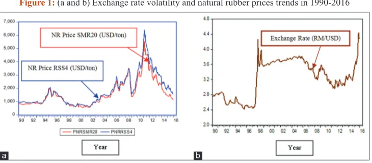
In terms of primary commodities, NR prices had risen from
USD2,000/tonne in September 2009 to USD5,500/tonne in February 2011 in Malaysia (Figure 1). Export volume had increased from 690 thousand tonnes to 960 thousand tonnes from 2009 to 2011. However, the NR prices had started to decrease
severely from USD2, 100 per tonne in January 2014 to USD1,100 per tonne in December 2015; the exchange rate was RM4.29 per USD during the period in Figure 1.
Figure 1 showed that the USD had depreciated against Malaysia’s currency and Malaysia’s real exchange rate had
started to decline from 1997-1998. When the NR price had
decreased but the exchange rate for Malaysia (RM/USD) had gone up, it meant that the exchange rate was still unstable, and it was creating that uncertainty over future price levels. It would complicate investment and discourage economic growth as the
NR price was extremely low again as experienced during the
estimating period in this study. Additionally, currency movements may show a discrepancy implication on competitiveness of the
external trade, debt, and foreign direct investment (NERP, 2014).
2. LITERATURE REVIEW
Osigwe and Uzonwanne (2015) suggested that there was a causality relationship between the foreign currency exchange rate and foreign direct investment (FDI). They used the unit root test for the stationary of the variables. They explained that all the variables became stationary at the first different level of the unit
root test. Then, the variables were long-run relationship among the variables by Johansen co-integration test. The causality showed
that unidirectional from foreign currency exchange rate and FDI at the lag section criteria mentioned the lag one to lag two
selections. Moreover, there was bidirectional causality between
foreign currency exchange rate and FDI at lag three selections.
Therefore, it provided the knowledge and idea to establish this
research methodology on the exchange rate volatility.
Jamil et al. (2012) investigated the exchange rate volatility on
the industrial production of common currency in the European Monetary Union. They used the data from the monthly data
collected from 1980 to 2009. The study used autoregressive EGARCH models for volatility analysis compared with nominal and real exchange rates. They found that all the industries were satisfied with the benefits after the introduction of common
currency and even some industries also looked increasing in
the exchange rate volatility. Thus, it could also provide that the
currency changes had affected for every country that had joined the trading of their productivities.
Oskooee and Harvey (2014) studied the role of the exchange rate
between the United States and Indonesia which traded agricultural commodities. Indonesia was the largest economy for trading the commodity in South East Asia. They estimated the currency depreciation on in-payments and out-payments in the trade. They
disaggregated the trade flows between US and Indonesia. The sensitivity of in-payments was 108 United State export industries
and out-payments were 32 United State import industries. They
investigated that most industries responded to the exchange rate changes in the short-term but some were significantly affected
in the long-term. This article endowed with the further study
methodology about Asian countries exchange rate currency.
Numerous old-fashioned theoretical studies as discussed by
an increase in exchange rate volatility exhibited adverse effects
on international trade volume.
Whereas, Doroodian (1999) stated that this effect can only show in developing countries. This view was also shared by (Hooper and Kohlagen, 1978) who constructed a static model of demand
and supply. Their results showed that the uncertainty of the
exchange rate had negative effects on volume share; however, the volatility of the exchange rate had positive effects on trade price. flow shows that product prices became unstable if the volatility of the exchange rate had increased drastically under the floating exchange rate system. Therefore, firms with risk aversed
tendencies tended to decrease trade volume thus this affected
real product prices. Simply put, the exchange rate volatility increased the exchange rate risk and thus reduced incentives of
international trade. It was commonly acknowledged that increased
exchange rate volatility restrained the growth of foreign trade. Negative effects of exchange rate uncertainty on trade flows supported the fact that exchange rate risk depressed trade flows (International Monetary Fund [IMF] (1984) and Clark et al. (2004). If movements in exchange rates became unpredictable, the profits made would be uncertain and, thus, depressed the benefits of international trade.
On the other hand, Thorbecke (2006) found that the exchange rate fluctuation would decrease Asian exports but export volume
was not guaranteed to increase if the U.S. dollar depreciated.
Therefore, the United States government should not expect the appreciation of Asian currencies to increase the export volume to the United States. Jarita (2008) tested the export and import price with the volatility of the exchange rate of the Malaysian ringgit from January 1999 to December 2006 via the vector error correction model (VECM). The results proved that the effects on export and import price from the volatility of the exchange rate were significant. On the contrary, a number of scholars think that exchange rate risk positively affected exports and imports with the explanation that exchange risk caused the substitution and
income effect.
Giovannini (1998) discovered that when the exchange rate risk increased, most risk-neutral traders entered the market quickly and
left the market slowly. The number of traders in the market would
increase, as will the trade volume. Bailey et al. (1986) assumed that traders could easily earn returns from the volatility of the exchange rate, coupled with knowledge of the trade. Franke (1991) proved that when the volatility of the exchange rate had increased, the cash flow from export increase was significantly greater than the entry and exit cost from the market for the trader who employed haphazard policies of entry and exit. De Grauwe (1988) & Broll and Eckwert (1999) proposed that the real options of export trade increased when the volatility of the exchange rate had increased.
The determinants of the NR price would affect the volatility
of NR (latex) price in Malaysia (Sadali, 2013). Describing the
high volatility in NR price, it was a relationship between the
international trade (export and import), inflation and crude oil price. The data utilized the monthly data collected from 1998-2012.
This paper tested the regression analysis and hypothesis testing between variables. The reason for the volatility of the NR price
was clearly explained with the crude oil price, inflation, export, and import. Sadali (2013) mentioned that the NR import was a
negative relationship between the prices. Also, it showed that crude oil price was a positive relationship with volatility of the price.
Based on the findings, if the NR raw materials are imported from
other countries, it would affect the decrease of the domestic NR
price and consequently affect the world NR price as well. Thus,
this article had also included the knowledge of the methodology
on how to find the factors affecting the volatility of NR price.
On the aspect of factors affecting the NR price, Raju (2016) stated
that synthetic rubber prices and crude oil prices affect NR prices
whereby the decline in oil prices and the subsequent decline
in the prices of synthetic rubber were some of the factors that have contributed to the volatility and instability in NR prices.
He explained that if the NR exporting countries were affected
by the economic slowdown especially with depreciation in the currencies and this was contributed to the decline in NR prices in these countries. This uncertainty will limit import capacity and thus result in lower investment and growth. The demand and supply volatility in both domestic and international markets could affect NR prices. In the case of NR, the domestic market is highly integrated with the international market. The instability
in the prices in the international market has significantly affected
the prices in the domestic market. Source: MRB, 2015: ANRPC (2016) and (BNM, 2016)
Figure 1: (a and b) Exchange rate volatility and natural rubber prices trends in 1990-2016
3. THEORETICAL FRAMEWORK AND
METHODOLOGY
With previous literature reviews of commodity price analysis, this
study focused on three issues in common: (i) The characteristics and
determinants of commodity price volatility; (ii) its macroeconomic effects and; (iii) the optimal policy responses to such volatility (Cashin et al., 2002; Deaton, 1999; Khin et al., 2011 and 2013). Based on the literature, in Equation 1, the forecasts of NR price (SMR20) of the study particularly would be the function of the substitute natural rubber price of RSS4 and exchange rate price (RM/ USD) (ERPM). A diagnosis checking for each variable is focused the
data series for the stationary, using unit root test of the Augmented
Dickey-Fuller (ADF) and Phillips-Peron’s tests (PP) (Gujarati & Porter, 2009; Studenmund, 2014). The causal relationship is first analyzed along the VECM model with more efficient causality procedure (Engle and Granger, 1991). Both short-term forecasts of ERP and NR prices of (SMR20 and RSS4) will be tested by using (Pindyck and Rubinfeld, 1998). Originally, a short-term NR price
VECM model mentioned as a function logs in below:
ΔPNRSMR20t = c0+a1PNRRSS4t−1+a2ERPMt−1+
a3PNRSMR20t−1+e1t (1)
Where:
PNRSMR20 = Price of natural rubber SMR20 in Malaysia (USD/tonne) deflated by the CPI
PNRRSS4 = Price of natural rubber RSS4 in India (USD/ton) deflated by the CPI
ERPM = Real exchange rate (Malaysia Ringgit (RM) per USD) (RM/USD)
T = Time trend monthly data from 1990 to 2015
ei = Error terms
Moreover, we can write the other variables’ VECM equations (2) and (3) as follows:
Δ PNRRSS4t = c1+a4ERPMt−1+a5PNRSMR20t−1+
a6PNRRSS4t−1+e2t (2)
Δ ERPMt = c2+a7PNRSMR20t−1+a8PNRRSS4t−1+a9ERPMt−1+e3t
(3)
cs = Intercept; as = The coefficients of the related factors
Research hypotheses:
H01: PNRSMR20 does not Granger cause PNRRSS4
HA1: PNRSMR20 Granger cause PNRRSS4
H02: PNRSMR20 does not Granger cause ERPM
HA2: PNRSMR20 Granger cause ERPM
H03: PNRRSS4 does not Granger cause PNRSMR20
HA3: PNRRSS4 Granger cause PNRSMR20
H04: PNRRSS4 does not Granger cause ERPM
HA4: PNRRSS4 Granger cause ERPM
H05: ERPM does not Granger cause PNRSMR20
HA5: ERPM Granger cause PNRSMR20
H06: ERPM does not Granger cause PNRRSS4
HA6: ERPM Granger cause PNRRSS4
Moreover, this study used the Johansen co-integration test to estimate the long-run relationship between the variables and co-integrated. It is a statistical concept of the regression theory
framework that described the long run equilibrium among the variables. Engle and Granger (1991) indicated that if a multiple
linear regression of two or more non-stationary series was
stationary, it was called the co-integrating equation and may be interpreted as a long-run equilibrium relationship among the variables. The Johansen co-integration equation for a short-term NR prices of (SMR20 and RSS4) and ERP is in Equation (4) as follows:
Co-integration: b1PNRSMR20t−1+b2PNRSS4t−2+b3ERPMt−3= 0 (4)
bs = The coefficients of the related factors
Engle and Granger (1991) found that the definition of causality
was being used to determine the direction and causality between the two variables. Eigenvalue:
PNRSMR20t= β1PNRSMR20t−1+β2PNRSMR20t−2+…
+βpPNRSMR20t−p
+α1PNRRSS4t−1+α2PNRRSS4t−2+…
+αp PNRRSS4t−p+u2,t (5)
PNRSMR20t= β3P N R S M R 2 0t − 1+ β4P N R S M R 2 0t − 2+ …
+βp PNRSMR20t−1+α3ERPMt−1+α4ERPMt−2+…
+αpERPMt−p+u2,t (6)
PNRRSS4t= β5PNRRSS4t−1+β6PNRRSS4t−1+…+βpPNRRSS4t−p + α5 P N R S M R 2 0t − 1+ α6P N R S M R 2 0t − 2+ …
+αpPNRSMR20t−p+u2,t (7)
PNRRSS4t= β7PNRRSS4t−1+β8PNRRSS4t−2+…+βpPNRRSS4t−p +α7 ERPMt−1+α8ERPMt−2+…+αpERPMt−p+u2,t (8)
ERPMt= β9ERPMt−1+β10ERPMt−1+…+βpERPMt−1+α9PNRRSS4t−1 +α10PNRRSS4t−2+…+αpPNRRSS4t−p+u2,t (9)
ERPMt= β1 1E R P Mt − 1+ β1 2E R P Mt − 2+ … + βpE R P Mt − p + α1 1P N R S M R 2 0t − 1+ α1 2P N R S M R 2 0t − 2+ …
+αpPNRSMR20t−p+u2,t (10)
αs = The coefficients of the related factors; βs = The coefficients
of the related factors.
4. EMPIRICAL RESULTS
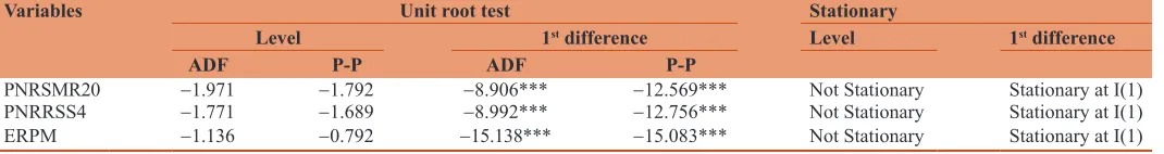
The results of the unit root test are presented in Table 1. The unit
root test was previously defined by Gujarati and Porter (2009). If the
formed for testing the unit root; H0: The time series data has unit
root (is non-stationary), and HA: The time series data has no unit root (is stationary). The PNRSMR20 price, PNRRSS4 price, and ERPM were non-stationary at levels I(0) i.e., they had a unit root. Therefore, they were made by using unit root test at the first differencing I(1) level to become stationary. Thus, the time series were stationary at the first differences I(1) at the 0.01 level. The unit root (stationary) for this study has been tested by utilizing the Augmented Dickey-Fuller (ADF) and Phillip-Perron (P-P). First, it checked both ADF and P-P unit root test “ t “ statistic value. It was (-) negative and indicated the “ t “ statistic value was bigger than the “MacKinnon critical values” at all three levels of significance. Also, if each of ADF and P-P unit root test “ t “ statistic’s p-value was as like (0.0000) also less than at α 0.05 statistically significant, the time series data is no unit root (stationary).
Accordingly, the vector correction model (VECM) of the short-term NR price (SMR20) results was explained in Equation (11). In equation (11), the NR price (SMR20) forecasting model was explained by 65 percent of the variation using the RSS4 NR price and exchange rate parameters. There is a short-run relationship between independent variables of RSS4 NR price, exchange rate, the lag variable of SMR20 NR price (PNRSMR20t−1) and dependent variable of SMR20 NR price (ΔPNRSMR20t) at α=0.01 and 0.05 level, respectively. Furthermore, the VECM model was
included together with the short-run relationship between the
variables and distributed lag variable. Therefore, (PNRSMR20t−1) is a distributed lag variable of ΔPNRSMR20t in this Equation (11). Moreover, the Breusch-Godfrey Serial Correlation LM test showed that residuals were significant at α=0.01 level and it meant that the
model had included the correct parameters. Residual diagnostics and parameter diagnostics contained the tools available for determining whether a selected model was valid.
ΔPNRSMR20t= 0.008+0.8694 PNRRSS4t−1−0.3073 ERPMt−1
t-statistics = [22.6708***] [−2.6483**]
−0.4423 PNRSMR20t−1+0.0119 e1t (11) [−3.8598**]
R2=0.6492 Adjusted R2 = 0.6469
Breusch-Godfrey serial correlation LM test
F-statistic = 1.5611 Prob. F(1,307) = 0.2125***
Obs*R2 = 1.5734 Prob. Chi-Square(1) = 0.2097***
Note: t-statistics in [ ], ***statistically significant at the 0.01 level, **at the 0.05 level, and *at the 0.10 level.
Based on the results, in Equation (12), the NR price (RSS4) VECM forecasting model was explained by 57 percent of the variation using the SMR20 NR price and exchange rate parameters. There
is also a short-run relationship between independent variables of
SMR20 NR price (PNRSMR20t), exchange rate and dependent variable of RSS4 NR price (Δ PNRRSS4t) at α 0.05 level, however, the lag variable of RSS4 NR price (PNRRSS4t−1) is not statistically significant.
ΔPNRRSS4t= 0.142+0.3863 PNRSMR20t−1−0.2190 ERPMt−1
t-statistics = [3.4817**] [−2.1724**]
−0.0339 PNRRSS4t−1+0.0155 e2t (12)
[−0.3118ns]
R2 = 0.5707 Adjusted R2 = 0.5611
Based on the results, Equation (13) is the output of the exchange rate volatility (ERPM) VECM model. In Equation (13), the exchange rate (ERPM) forecasting model was explained by 54 percent of the variation using the SMR20 and RSS4 NR price parameters. There
is also a short-run relationship between independent variables of
SMR20 NR price (PNRSMR20t), RSS4 NR price (PNRRSS4t−1), the lag variable of exchange rate (ERPMt−1) and dependent variable of exchange rate (Δ ERPMt) at α = 0.05 level, respectively.
ΔERPMt=0.013−0.0291 PNRSMR20t−1−0.0287 PNRRSS4t−1−
t-statistics = [−4.7035**] [−4.7501**]
0.2632 ERPMt−1+0.0051 e3t (13)
[−4.2145**]
R2 = 0.5496 Adjusted R2 = 0.5398
After they were given the unit root test in I(1), they were tested for Johansen co-integration Equation (14) and test in Table 2.
The Johansen co-integration equation for a short-term NR prices of (SMR20 and RSS4) and ERP is in Equation (14) as follows:
Co-intEquation: 0.2927 PNRSMR20t−1−0.5096 PNRSS4t−1 t-statistics = [−2.4456**] [−4.8520**]
+0.1929 ERPMt−1=0 (14)
[−5.3604***]
Therefore, based on Equation (14), there is a long-term relationship between NR price (SMR20) (PNRSMR20t−1), RSS4 (PNRSS4t−1) and exchange rate (ERPMt−1) at α 0.05 and 0.01 level statistically significant and they are co-integrated each other in Table 2.
Table 1: Unit-root tests for exchange rate and Malaysian NR prices
Variables Unit root test Stationary
Level 1st difference Level 1st difference
ADF P-P ADF P-P
PNRSMR20 ‑1.971 ‑1.792 ‑8.906*** ‑12.569*** Not Stationary Stationary at I(1)
PNRRSS4 ‑1.771 ‑1.689 ‑8.992*** ‑12.756*** Not Stationary Stationary at I(1)
Table 2 shows Ho: There are no long-run and co-integration relationship between the variables. HA: There is long-run and
co-integration relationship between the variables at the 5% and 1% level. It is based on P-values (5% and 1% level) of Eigenvalue
and Trace Statistic. Eigenvalue and Trace statistics indicate 3
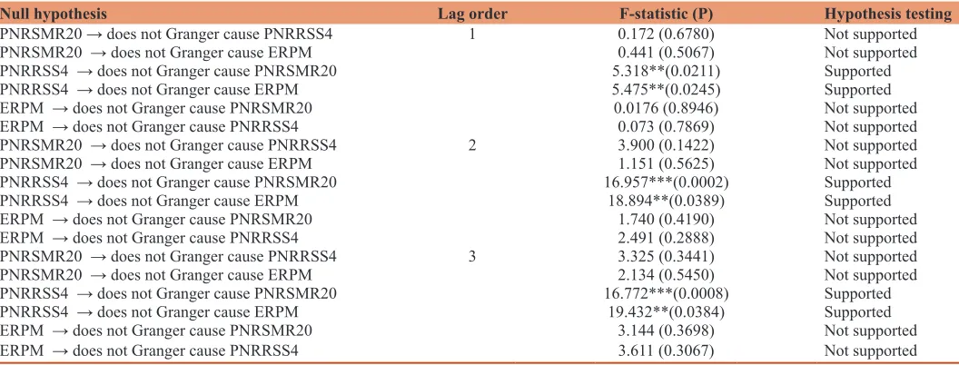
cointegrating equations significant long-run relationship at the 0.05 and 0.01 level. This means that there is a long-run relationship between NR prices of PNRSMR20 price, PNRRSS4 price, and ERPM exchange rate. Evidence of co-integration suggested the granger causality (Table 3) also showed Ho: PNRSMR20 does not Granger cause to PNRRSS4 and HA: PNRSMR20 Granger causes PNRRSS4 and so on. The results mentioned that one direction (unidirectional causality) from PNRRSS4 price to PNRSMR20 price; and from PNRRSS4 price to ERPM exchange rate at lag
order 1, 2 and 3.
It indicated that if RSS4 price had high instability, it created
volatility of SMR20 price as well as the exchange rate. Otherwise, the Malaysian NR price (SMR20) are related to increase or
decrease based on the world NR prices such as India rubber price
(RSS4), Shanghai rubber price, Japan rubber price (TOKOM), Singapore rubber price (SICOM) and so on (ANRPC, 2016). Also, currency exchange rate volatility can affect the NR price because most agricultural commodities are traded in USD. Osigwe and Uzonwanne (2015) analyzed also the Granger causality of foreign reserves, exchange rate and foreign direct investment (FDI). All of the variables were non-stationary at levels I(0) and became stationary after the first differences I(1). Moreover, the result
proved that there was a long-run relationship among the variables
and the Granger causality test which indicated unidirectional causality from exchange rate to other variables at lag order 1 and 2.
Cashin et al. (2004) explained that the real exchange rates of commodity-exporting countries and the real prices of their commodity exports had instability together over time. There was also a long-run relationship between real exchange rate and real commodity prices. They proved that the long-run real exchange rate and the prices of export commodities were not constant. Also, Dauvin (2014) used the cointegrating relationship between the real exchange rate and oil prices. He investigated the relationship between energy prices (oil prices) and the real effective exchange rate of commodity-exporting countries. He found that increased
commodity price volatility caused the uncertainty the future
exchange rate and it may affect the countries’ economic growth.
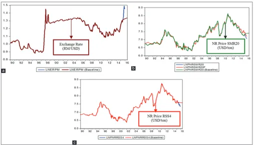
Figure 2 described both short-term NR prices (PNRSMR20 and PNRRSS4) and ERPM ex-ante forecasts would be slightly increasing trend from January to June 2016.
5. CONCLUSION
This study determined the impact of exchange rate volatility on both NR prices of (SMR20 and RSS4); and predicted the forecast of a short-term exchange rate (RM per USD) and both NR prices (SMR20 and RSS4) strongly represented in the Malaysian NR market. The results showed that between RSS4 price, SMR20 and ERP were a Granger-cause and unidirectional relationship. Both short-term NR prices and ERPM ex-ante forecasts would be a slightly increasing trend from January to June 2016. It may
be due to the government and traders in changing their behaviour
by increasing domestic consumptions for the stabilization of the NR supply-demand balance. Products like rubber tires, footwear, gloves, condoms and catheters of rubber products and latex products
Table 2: Johansen’s co-integration test (intercept and no trend)
Hypothesized No. of CE (s) Eigen value Trace statistic 0.05 critical value P-value 0.01 critical value P-value
None* 0.3969 350.7542 29.7971 0.0001 35.4582 0.0001
At most 1* 0.3272 194.4782 15.4947 0.0001 19.9371 0.0001
At most 2* 0.2079 72.0246 3.8415 0.0000 6.6349 0.0000
Eigen and Trace statistics indicate 3 cointegrating eqn (s) at the 0.05 and 0.01 level. *denotes rejection of the hypothesis at the 0.05 and 0.01 level; **MacKinnon-Haug-Michelis (1999) P values
Table 3: Granger causality analysis and hypotheses testing decision
Null hypothesis Lag order F-statistic (P) Hypothesis testing
PNRSMR20 → does not Granger cause PNRRSS4 1 0.172 (0.6780) Not supported
PNRSMR20 → does not Granger cause ERPM 0.441 (0.5067) Not supported
PNRRSS4 → does not Granger cause PNRSMR20 5.318**(0.0211) Supported
PNRRSS4 → does not Granger cause ERPM 5.475**(0.0245) Supported
ERPM → does not Granger cause PNRSMR20 0.0176 (0.8946) Not supported
ERPM → does not Granger cause PNRRSS4 0.073 (0.7869) Not supported
PNRSMR20 → does not Granger cause PNRRSS4 2 3.900 (0.1422) Not supported
PNRSMR20 → does not Granger cause ERPM 1.151 (0.5625) Not supported
PNRRSS4 → does not Granger cause PNRSMR20 16.957***(0.0002) Supported
PNRRSS4 → does not Granger cause ERPM 18.894**(0.0389) Supported
ERPM → does not Granger cause PNRSMR20 1.740 (0.4190) Not supported
ERPM → does not Granger cause PNRRSS4 2.491 (0.2888) Not supported
PNRSMR20 → does not Granger cause PNRRSS4 3 3.325 (0.3441) Not supported
PNRSMR20 → does not Granger cause ERPM 2.134 (0.5450) Not supported
PNRRSS4 → does not Granger cause PNRSMR20 16.772***(0.0008) Supported
PNRRSS4 → does not Granger cause ERPM 19.432**(0.0384) Supported
ERPM → does not Granger cause PNRSMR20 3.144 (0.3698) Not supported
ERPM → does not Granger cause PNRRSS4 3.611 (0.3067) Not supported
selling industries and rubberwood products selling furniture
industries, which use raw materials and export the rubber products in US dollars, would have benefited from this study’s findings. Significantly, it is also encouraged that information be available
for Malaysian rubber industries because they are still producing
positive net trade flows, provide steady employment and consistent
earnings for the government. For further studies, authors are willing to do the comparative forecasting accuracy by using univariate
Autoregressive Integrated Moving Average (ARIMA), simultaneous system equation, and Autoregressive Conditional Heteroskedasticity (ARCH) type models with stationarity test. It would be directly
considered in enhancing the validity of the current studies and
providing new evidence on the impact of exchange rate volatility and
comparative forecasting accuracy among the models. It will be based
on the Root Mean Squared Error (RMSE), the Mean Absolute Error (MAE), the Root Mean Percent Error (RMPE) and Theil’s inequality coefficients (U-Theil) criteria towards Malaysia’s commodity
trading with the other natural rubber producing countries.
6. ACKNOWLEDGEMENT
This research paper is under the funding of the Universiti Tunku
Abdul Rahman (UTAR)’s Internal Research Fund (UTARRF) and the authors greatly express deep appreciation to UTAR which has
provided funding for this research.
REFERENCES
ANRPC. (2016), Natural Rubber Daily and Weekly Prices. Available from: http://www.anrpc.org/html/daily_prices.aspx.
Bailey, M.J., Tavlas, G.S., Ulan, M. (1986), Exchange-rate variability and
trade performance: Evidence for the big seven industrial countries. Weltwirtschaftiliches Archiv, 122, 466-477.
Bank Negara Malaysia (BNM). (2016), Historical Chart of Euro Currencies.
http://www.bnm.gov.my/index.php?ch=statisticandpg=stats_ exchangerates.
Broll, U., Eckwert, B. (1999), Exchange rate volatility and international
trade. Southern Economic Journal, 66, 178-185.
Budiman, A.F.S., Fortucci, P. (2003), Consultation on Agricultural Commodity Price Problems, 25-26 Mar 2002. FAO, Rome (Italy): Commodities and Trade Div. Available from: http://www.fao.org/ docrep/006/y4344e/y4344e0d.htm.
Burger, K., Smit, H.P., Vogelvang, B. (2002), Exchange Rates and Natural Rubber Prices, the Effect of the Asian Crisis. Vrije University, Faculty
of Economics and Business Administration, Economic and Social
Institute, Department of Econometrics.
Cashin, P., Céspedes, L.F., Sahay, R. (2004), Commodity currencies and the real exchange rate. Journal of Development Economics, 75(1),
239-268.
Cashin, P., McDermott, C.J., Scott, A. (2002), Booms and slumps in world commodity prices. Journal of Development Economics, 69, 277-296. Clark, P.B., Tamirisa, N., Wei, S.J. (2004), Exchange Rate Volatility and
Trade Flows-some New Evidence (International Monetary Fund Policy Paper). Washington, DC: International Monetary Fund. p19. Corden, W.M. (1993), Exchange rate policies for developing countries.
The Economic Journal, 103(416), 198-207.
Dauvin, M. (2014), Energy prices and the real exchange rate of commodity-exporting countries. International Economics, 137,
52-72.
De Grauwe, P. (1988), Exchange Rate Variability and the Slowdown in Growth of International Trade, IMF Staff Paper, 35, 63-84. Deaton, A. (1999), Commodity prices and growth in Africa. Journal of
Economic Perspectives, 13(3), 23-40.
Doroodian, K. (1999), Does exchange rate volatility deter international trade in developing countries? Journal of Asian Economics, 10(3),
465-474.
Figure 2: (a-c) Short-term ex-ante forecasts of both natural rubber (NR) prices (log data) and exchange rate (log data) in the Malaysian NR market
c
Drabek, Z., Brada, J.C. (1998), Exchange rate regimes and the stability
of trade policy in transition economies. Journal of Comparative
Economics, 26(4), 642-668.
Engle, R.F., Granger, C.W.J. (1991), Long-run Economic Relationships: Readings in Cointegration. Oxford: Oxford University Press. Ethier, W. (1973), International trade and the forward exchange market.
American Economic Review, 63(3), 494-503.
Evenett, S.J., Jenny, F. (2012), Commodity prices, government policies
and competition. In: Steve, M., editor. Trade, Competition, and
the Pricing of Commodities. London: Centre for Economic Policy Research and Consumer Unity and Trust Society (CUTS International). p3-30.
Franke, G. (1991), Exchange rate volatility and international trading strategy. Journal of International Money and Finance, 10(2), 292-307. Giovannini, A. (1988). Exchange rate and traded goods prices. Journal
of International Economics, 24, 45-68.
Goldberg, L., Charles, K. (2005), Foreign direct investment, exchange
rate variability and demand uncertainty. International Economic
Review, 36(4), 855-873.
Gujarati, D.N., Porter, D.C. (2009), Basic Econometrics. 5th ed. New
York: McGraw-Hill.
Hooper, P., Kohlagen, S.W. (1978), The effects of floating exchange rate
uncertainty on the price and volume of international trade. Journal of International Economics, 8, 483-511.
International Monetary Fund. (1984), Exchange Rate Volatility and World Trade (International Monetary Fund Occasional Paper No. 28). Washington, DC: International Monetary Fund.
Jamil, M., Streissler, E.W., Kunst, R.M. (2012), Exchange rate volatility
and its impact on industrial production, before and after the introduction of unstable currency in Europe. International Journal
of Economics and Financial Issues, 2(2), 85-109.
Jarita, D. (2008). Impact of Exchange Rate Shock on Prices of Imports and Exports, Munich Personal RePEc Archive Working Paper. Khin, A.A., Zainalabidin, M., Amna, A.A.H. (2013), The impact of the
changes of the world crude oil prices on the natural rubber industry
in Malaysia. World Applied Sciences Journal, 28(7), 993-1000.
Khin, A.A., Zainalabidin, M., Shamsudin, M.N., Eddie, C.F.C., Arshad, F.M. (2011), Estimation methodology of short-term natural
rubber price forecasting models. Journal of Environmental Science
and Engineering, 5(4), 460-474.
Malaysia Rubber Board (MRB). (2015), Natural Rubber Statistics. Malaysia: Malaysian Rubber Board; 2015. Available from: http:// www.lgm.gov.my/nrstat/nrstats.pdf; Available from: http://www3. lgm.gov.my/Digest/digest/ digest-12-2015.pdf.
National Economic Recovery Plan (NERP). (2014), The Crisis and Policy Response, Effects of the Crisis. The National Economic Action Council (NEAC). Malaysia: Economic Planning Unit, Prime Minister’s Department. Available from: http://www.mir.com.my/lb/ econ_plan/contents/chapter1/a_pg6.htm.
Osigwe, A.C., Uzonwanne, M.C. (2015), The causal relationship between foreign reserves, exchange rate, and foreign direct investment:
Evidence from Nigeria. International Journal of Economics and
Financial Issues, 5(4), 884-888.
Oskooee, M.B., Harvey, H. (2014), US-Indonesia trade at commodity level and the role of the exchange rate. Applied Economics, 46(18),
2154-2166.
Peree, E., Steinherr, A. (1989), Exchange rate uncertainty and foreign
trade. European Economic Review, 33, 1241-1264.
Pindyck, R.S., Rubinfeld, D.L. (1998), Econometric Models and
Economic Forecasts. 4th ed. New York: McGraw-Hill Companies,
Inc.
Raju, K.V. (2016), Instability in natural rubber prices in India: An empirical analysis. IOSR Journal of Economics and Finance (IOSR-JEF), 7(3), 24-28.
Sadali, N.H. (2013), The Determinant of Volatility Natural Rubber Price. Available from: http://www.ssrn.com/abstract=2276767.
Studenmund, A.H. (2014), Using Econometrics: A Practical Guide. 6th ed.
Pearson: Prentice Hall.
Thorbecke, W. (2006), The Effects of Exchange Rate Changes on Trade in East Asia, REITI Discussion Paper Series Working Paper. UNCTAD. (2011), Price Volatility in Food and Agricultural Markets: