Technology Shocks and Asset Pricing:
The Role of Consumer Con…dence
Vincenzo Merellay Stephen E. Satchellz
October 2014
Abstract
We show that the introduction in a power utility function of a con…dence index to signal
the state of the world allows for an otherwise standard asset pricing model to match the observed consumption growth volatility and excess returns with a reasonable level of relative risk aversion. Our results stem from two quantitative exercises: a calibration and a
non-linear estimation. In both cases, our …ndings are robust to di¤erent data frequencies and various indicators of con…dence. Our estimations are also robust to a number of instrument speci…cations. We rationalise this …nding by developing a model where monopolistically
competitive …rms are subject to idiosyncratic shocks, which a¤ect both the quantity and the quality of the goods produced. When households foresee good times, they expect …rms to generate higher pro…ts and produce higher quality goods. While greater expected excess returns provide a larger incentive to save, better expected quality of consumption discourages
saving, as it lowers the expected marginal utility of any given level of physical consumption. Compared to standard consumption-based frameworks, our model thus predicts a more stable consumption path. Our analysis suggests that con…dence provides a suitable proxy for the
unobservable quality of consumption via the positive links between these two variables and the overall performance of the economy. Furthermore, the observed predictive power of con…dence on consumption growth might be justi…ed by the interplay of qualitative and
quantitative aspects of consumption in the Euler equation rather than by the customary notion of con…dence as household expectation of the future state of the economy.
JEL Classi…cation: G12, E21
Keywords: Asset Pricing, Consumer Con…dence, Product Quality, Technology Shocks We would like to thank Henrique Basso, Michele Boldrin, Esteban Jaimovich, Monika Junicke, Miguel Leon-Ledesma, Alessio Moro, David Webb and Stephen Wright for their helpful advice and all participants to the Birkbeck seminars in London, to the DECA seminar in Cagliari, to the Collegio Carlo Alberto seminar in Turin, to the University of Kent seminar in Canterbury, to the 4th International Conference in Bilbao, and to the 48th SIE Conference in Turin for their useful comments.
yUniversity of Cagliari and BCAM, Birkbeck, University of London. Email: [email protected].
1
Introduction
The …nancial markets, the media and the business community interpret the indices of consumer
con…dence as indicators of changes in household income or wealth. Higher con…dence, the typical
story goes, signalling better economic conditions, makes agents feel richer and, accordingly,
consume more. A number of academic articles appear to endorse this view. Empirical evidence
suggests that consumer con…dence predicts consumption growth, over and above other commonly
used economic indicators (for a discussion, see,e.g., Ludvigson, 2004).
The link between con…dence and consumption growth is particularly interesting in
conjunc-tion with the poor performance of the consumpconjunc-tion-based asset pricing models. A long list of
papers show that the existing asset pricing theories fail to match risk-free returns and equity
premia with consumption growth volatility, when a power utility function represents household
preferences. Economists have attempted to solve this issue by generalising the utility function,
while retaining the attractive properties of its power speci…cation. The leading contributions in
this literature suggest introducing time non-separability in consumption, or positing that utility
is a function of consumption and some other good. None of these attempts, however, appear
to decisively improve the ability of the consumption-based model to …t the data: implausibly
large values of either risk aversion or intertemporal elasticity of substitution are required for
the model to match risk-free returns and equity premia with consumption growth volatility (for
recent surveys of this literature, see, e.g., Ludvigson, 2012; and Mehra, 2012).
In this paper, we investigate whether taking into account con…dence indicators may improve
the empirical performance of the consumption-based asset pricing model. In Section 2, we
develop a model to formalise our hypothesis. As in several other contributions in the literature,
our model features an unobservable state variable that in‡uences the magnitude of marginal
utility of consumption, and thereby the value of the stochastic discount factor that prices assets.
The state variable magni…es utility (and lowersmarginal utility) of any given consumed quantity
in good times, and has the opposite e¤ect in bad times. If the state variable correlates positively
with the performance of the economy, then risky assets payo¤s tend to be large when marginal
utility of consumption is lower than in the benchmark model, and vice versa. As a result, in
this case consumption is less responsive to …nancial incentives.
The novel feature of our approach is that consumer con…dence is used as a proxy for the
unobservable state variable. Our intuition, discussed in Section 3, builds on two arguments. On
the one hand, the state variable in‡uences household utility and, as such, may re‡ect aspects of
the consumption experience that are not captured by a quantitative measure of consumption:
in particular, some elements characterising the goods consumed (e.g., consistency with
pre-purchase expectancy, reliability, freshness, etc.). On the other hand, consumer con…dence is
the aggregate outcome of producers’ performances: these performances may in‡uence goods’
attributes, and thereby have a signi…cant impact in shaping consumption experience. Hence,
consumer con…dence may o¤er an indirect indication of the degree of satisfaction that households
experience when consuming a given quantity of goods.1
In our quantitative model, we accordingly use consumer con…dence as a proxy for the state
variable. The stochastic discount factor is then determined by a function of the growth factors of
con…dence and consumption. We calibrate the Euler equation resulting from our model, and also
test it empirically using method-of-moments estimation. Section 4 illustrates our quantitative
and empirical results. Both exercises show that our model is able to match the observed asset
returns and consumption growth volatility with plausible values of risk aversion, when consumer
con…dence is used as a proxy for the unobservable state variable. Our …ndings are robust to
di¤erent data frequencies and various indicators of con…dence. Our estimations are also robust
to a number of instrument speci…cations.
Naturally, we are well aware of Fama’s (1991) criticism to models that “search the data
for variables that, ex post, describe [...] average returns.” For this reason, Section 5 proposes
a theoretical rationale for the introduction of the state variable. Our explanation refer to the
qualitative dimension of consumption, which is generally unobservable in the data, and thereby
neglected by several branches of the economic literature. In a nutshell, our intuition is that
‘positive’ states (high consumer con…dence) may be signalling better quality of consumption.
A number of contributions suggest that the qualitative dimension of consumption may be an
important driver of households’decisions, particularly in rich economies (see,e.g., Fajgelbaum,
Grossman and Helpman, 2011; and Jaimovich and Merella, 2012). Though obtaining an observed
measure of the quality level of domestic aggregate consumption is virtually impossible, from
these studies we learn that quality of consumption is tightly linked with the performance of the
economy. Building on the arguments discussed in Section 3, the fact that con…dence indicators
are designed to re‡ect precisely the households’ view about the performance of the economy
suggests that consumer con…dence may represent an indirect proxy for consumption quality.2
1In particular, our interpretation of con…dence as a proxy for households’satisfaction in consumption is based on the Present Situation Indicator, one of the two components of Conference Boards’Consumer Con…dence Index. Economists typically disregard that indicator, since the observed predictive power on consumption growth appears to result from its Expectations counterpart (see, e.g., Ludvigson, 2004). We show that the Present situation component is nevertheless a robust indicator of households’ view on the overall performance of the economy. Furthermore, we argue that our intepretation is suggestive of to a novel rationale for the link between con…dence and consumption growth, based on qualitative aspects of consumption rather than future income expectations.
2
Related literature
A number of contributions attempt to explain the observed correlation between current
con-sumer con…dence and future consumption growth. Two main ideas are investigated in this
literature. The …rst is that, in line with the common wisdom, con…dence may capture household
expectations of future income or wealth, which might also be suggestive of a potential role for
habit formation.3 We depart from this view by opting for a more literal reading, which simply posits that consumer con…dence captures the household view on the performance of the
econ-omy. Building on our reasoning that links economic performance and the qualitative level of
consumption, we argue that con…dence indirectly signals a shift in the utility value achievable
with any given level of expenditure, rather than a change in the spending capabilityper se. The
second idea is that consumer con…dence re‡ects uncertainty. As such, it might alter
precaution-ary savings motives, owing to changes in the forecast variance of consumption.4 Our approach di¤ers in that con…dence does not a¤ect uncertainty in terms of consumption capability, but
rather expresses variations in its utility value.
From a quantitative point of view, this paper refers to the vast literature attempting to resolve
the equity premium and interest rate puzzles.5 In particular, it relates to those contributions that have appealed to preference modi…cations. Most of these articles suggest either to disentangle
relative risk aversion and intertemporal elasticity of substitution, or to introduce habit formation
in consumption.6 Our approach di¤ers in that we retain the standard single-coe¢ cient power economic transactions (e.g., about 16.5% of the U.S. GDP in the period 2008-2011), this strategy would hardly produce a reliable measure.
3
This hypothesis …nds little support in the data. Ludvigson (2004) shows that consumer con…dence has some forecasting power for future labour income growth and non–stock market wealth growth, although this predictive power is not just con…ned to an indirect e¤ect through household income or wealth. Carroll, Fuhrer and Wicox (1994) claim that the presence of habit formation, which implies that lagged consumption growth has predictive power for current consumption growth, might explain the correlation of lagged con…dence with current consumption growth as arising from the correlation of lagged con…dence with lagged consumption growth. Lagged consumption growth, however, is always included in their instrument sets. Thus, under their hypothesis, con…dence should have had no incremental explanatory power.
4
The relevant evidence is mixed. On the one hand, using UK data, Acemoglu and Scott (1994) …nd that high consumer con…dence signals both higher consumption growth (savings accumulation) and a higher forecast variance (uncertainty), which suggests a positive link between saving and uncertainty. On the other hand, Carroll
et al. (1994) and Ludvigson (2004) …nd a negative correlation between con…dence and uncertainty in US data, and argue that precautionary saving motives would lead to a positive relationship between consumption growth and lagged uncertainty, which would contradict the observed positive correlation between con…dence and consumption growth.
5
The equity premium puzzle (EPP), …rst described by Mehra and Prescott(1985), arises empirically when asset prices are related to household saving decisions. The magnitude of the puzzle is measured by the di¤erence between the value of the relative risk aversion required by asset pricing models (at least as large as twenty, see also Makiw and Zeldes, 1991) and that estimated by microeconometric works (just in excess of two, seee.g. Blume and Friend, 1975; Pratt and Zeckhauser, 1987). The interest rate puzzle, pointed out by Weil (1989), closely relates to the EPP, and refers to the large di¤erence between the observed risk-free returns and those predicted by consumption-based asset pricing models.
speci…cation, and postulate that utility is statically nonseparable in the quantity and the quality
of the goods consumed rather than time-nonseparable in consumption. A smaller branch of
the literature deviates from the view that …nancial risk is the sole force driving consumption
decisions, and postulates that utility is a function of consumption and some other good.7 We depart from this view by specifying preferences with exclusive regard to (the di¤erent aspects
of) consumption.
From a theoretical point of view, the distinctive feature of the present model is that
idio-syncratic technology shocks in‡uence marginal utility of consumption by altering the quality
level of the goods consumed. In this sense, our approach di¤ers from the works of Lucas (1992)
and Atkeson and Lucas (1992), who adopt aggregate taste shocks; and from that of Bencivenga
(1992), who introduces shocks to aggregate consumption and leisure. It also complements the
contributions by Horvath (1998, 2000), who introduces sectoral productivity shocks while
ab-stracting from preference shocks.8 Our model also relates to the setup in Busato (2004), who introduces the concept of relative demand shocks into a business cycle model while abstracting
from productivity shocks.
2
The model
We begin our analysis by developing a simple consumption-based asset pricing model in which
household preferences are state-dependent. For now, we just assume that household utility is
a function of the product between aggregate consumption and the state variable. The rest of
our framework is analogous to the typical model: household preferences are represented by a
power utility function; two assets, one risk-free and the other state-contingent, are traded; free
portfolio formation and the law of one price hold. In the next section, we discuss our choice for
the proxy of the unobservable state variable introduced here. Later, Section 5 o¤ers a rationale
for the particular way we formalise the introduction of the state variable.
Let household intertemporal preferences be represented by an additively separable power
utility, de…ned over the stream of present and future products between the state variable tand
aggregate consumptionXt, and formally given by:
U =E0 (
X
t2N
t( tXt)1 1
)
; (1)
authors consider to depart from full raitonality: e.g., Cochrane (1989); Cecchetti, Lam and Mark (2000). 7See, e.g., Eichenbaum, Hansen and Singleton (1988), who suggest leisure; Aschauer (1985), who proposes government spending; Startz (1989), who advocates the stock of durable goods; and, more recently, Finkelstein, Luttmer and Notowidigdo (2013), who posit health indicators.
8
where: t indicates time; E0 denotes the expectation operator conditional on the information available at date 0; > 0 is the household subjective discount factor; > 1 measures the curvature of one-period utility.9
At each date t, households are endowed withwt units of resources, which they can transfer over time by trading two types of assets: equities, whose holdings are denoted by At+1, which provide a state-contingent real rate of returnrA;t+1;bonds, whose holdings are denoted byBt+1, which ensure a real rate of returnrB;t+1. Equities pay the holder (stochastic) dividends. Pro…ts are distributed each period, hence dividends equal pro…ts.
The representative household chooses the value for the stream of consumption indicesfXtgt2N in order to maximize utility (1), subject to the intertemporal budget constraint:
Xt=wt At+1+ (1 +rA;t)At Bt+1+ (1 +rB;t)Bt: (2)
The household problem can thus be formally stated as follows:
max fXtgt2N
U =E0 (
X
t2N
t( tXt)1 1
)
;
subject to: Xt=wt At+1+ (1 +rA;t)At Bt+1+ (1 +rB;t)Bt:
(3)
The dynamics of our model economy are driven by a pair of shocks. A technology shock
"at a¤ects equity returns, which evolve according to the function rA;t = re" a
t, where r E0(rA;t). A preference shock "t a¤ects the state variable through the equation t=e"t, hence
E0( t) = 1. We assume that the two shocks are i.i.d. over time, but display a positive (simultaneous) correlation: "a;" > 0.10 The positive link between the overall performance of the economy and the state variable implies that utility of any given level of consumption,
measured by ( tXt)1 =(1 ), tends to be magni…ed by t in good times, and reduced in bad times, whereas marginal utility of consumption, measured by ( t)1 (Xt) , has the opposite response, decreasing in good times and increasing in bad times.
The in‡uence of the state variable on the optimal intertemporal consumption path formally
works through the Euler equation, which solves problem (3), and from which we obtain the
9By assuming that the household has power utility, the relative risk aversion (RRA) coe¢ cient is automatically tied to the consumption intertemporal elasticity of substitution. More precisely, the relative risk aversion coe¢ -cient is given by the reciprocal of the elasticity of the marginal utility of consumption with respect to consumption,
i.e.:
RRA "U0(Xt);Xt 1
= U
00(X t)Xt U0(Xt) = :
The assumption >1follows from the fact that the value of the RRA coe¢ cient is estimated to be in excess of two. See,e.g., Blume and Friend (1975); and Pratt and Zeckhauser (1987).
optimal distribution of resources over time:11
E0 "
1 +rA;t+1 1 +rB;t+1
t+1 t
1
Xt+1 Xt
# =E0
"
t+1 t
1
Xt+1 Xt
#
: (4)
We can draw two conclusions from inspection of the equilibrium condition expressed by (4). On
the one hand, for a given value of the state variable, household choice is standard. Expected
future high returns 1 +rA;t+1 induce households to increase the demand for equities, giving up some units of either current consumption Xt or bonds Bt (or both). As a result, larger expected future returns imply higher expected consumption growth. On the other hand, given
equity returns, variations in the state variable entails the following mechanism. Higher expected
values of the state variable lower the expected marginal utility of consumption. The household is
induced to adjust its consumption pattern by raising current relative to future consumption. As
a result, higher expected values of the state variable implylower expected consumption growth.
As we show below, the correlations between equity returns and each con…dence indicator
are positive (and in line with what is assumed above).12 Taken together, the two conclusions just sketched then imply that the e¤ect of the expected value of the state variable on household
choice tend to balance out the in‡uence of expected returns, and consumption is predicted to
‡uctuate less than in models where the state variable is absent. Section 4 assesses this prediction
quantitatively. In the next section, we explain the reasons for choosing consumer con…dence to
’quantify’the unobservable state variable when bringing the model to the data.
3
The role of consumer con…dence
As far as the model of the previous section is concerned, there is no obvious way to …nd a direct
measure the state variable in the data. We therefore need to identify some indirect proxy
for it: we choose the indicators of consumer con…dence. As we mentioned in the introduction,
the intuition behind this choice builds on a number of considerations. First, we postulate that
the state variable re‡ects the level of satisfaction in the consumption experience due to other
aspects than the quantity consumed. Second, given that …rm performances govern at least
some elements in‡uencing the consumption experience, on aggregate this level of satisfaction
correlates positively with the state of the economy. Third, consumer con…dence is designed to
reveal the households’perception of the state of the economy. Jointly taken, these considerations
suggest that consumer con…dence may o¤er an indirect indication of the degree of satisfaction
of consuming a given amount of goods.
A formal theoretical rationale for our reading of the state variable will be discussed in Section
1 1
For the complete derivation of (4), see Appendix B. 1 2
5. Here, we focus on the more practical matter of understanding whether, and if so which,
indicator of consumer con…dence depicts a households’view of the performance of the economy
that suits our interpretation of proxy for the state variable. In particular, we seek an indicator
that portrays the state of the economy ‘in absolute terms’, asking respondents to evaluate the
economic situation at a given point in time rather than to compare it at two di¤erent dates.
The reason for this is that we ultimately aim to capture a signal, brought forth by consumer
con…dence via the correlated variation in the consumption experience, that is contemporaneous
to the household decision on the quantity consumed.
Several indicators measure U.S. consumer con…dence or similar concepts. Among them,
two in particular have attracted the attention of academics: the Conference Board’s Consumer
Con…dence Index (CC), and the University of Michigan’s Consumer Sentiment Index (CS).
They display similarities (both are based on …ve questions; and have two sub-components: a
two-question component related to the present situation, and a three-question expectations
component) as well as distinctive features (sample sizes of about 3500 and 500 individuals,
respectively; di¤erent survey and aggregation procedures, etc.).13 Since the …rst indicator asks respondents to evaluate the economic situation at a given point in time while the second asks
for a comparison at two di¤erent dates, we focus on the Conference Board’s index to construct
our argument linking con…dence to the household perception of the state of the economy.14 The Conference Board de…nes the Consumer Con…dence Index as “a barometer of the health
of the U.S. economy from the perspective of the consumer.”15 The …ve questions asked to the respondents are:
1. “how would you rate present general business conditions in your area? [good/normal/bad]”
2. “what would you say about available jobs in your area right now? [plentiful/not so
many/hard to get]”
3. “six months from now, do you think business conditions in your area will be [better/same/
worse]?”
4. “six months from now, do you think there will be [more/same/fewer] jobs available in your
area?”
5. “how would you guess your total family income to be six months from now [higher/same/
lower]?”
1 3
For a thorough analysis of the two indicators, we refer to Bram and Ludvigson (1998). 1 4
In particular, the Consumer Sentiment Index features an heterogeneous “timing” in formulating the relevant questions, which include comparison to one year lag in the past and to a one to …ve years in the future.
The …rst two questions constitute the present situation component (CCP), and portray the
households’ view on the level of the current economic conditions. The remaining three
ques-tions comprise the expectaques-tions component (CCE), and depict the household’s projection of the
variation of the state of the economy relative to the current condition.16
The present situation component can be interpreted as the households’ assessment of the
current performance of the economy. As such, current CCP represents a natural candidate to
re‡ect the households’ perception on the realised state of the economy, and thus a possible
proxy for t. The expectations component can be thought of as re‡ecting the information that
households at present possess about the change in the future realisation of CCP, relative to
the current one. As such, current CCE may represent a possible proxy for t+1= t, once the benchmark for this change (i.e., the value of tor, in quantitative terms, the current realisation
of CCP) is properly accounted for. As we discuss in the next paragraph, households appear to
be observationally capable to produce good forecasts of the variations in the future realisation
of CCP, we opt for using CCP variation as our leading variable to choose the proxy for t+1= t, rather than constructing a composite index based on information from the lagged realisations
of CCP and CCE, whose functional form would be arbitrary by construction.
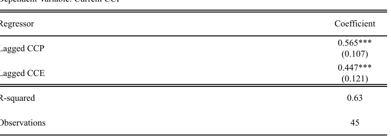
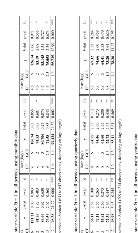
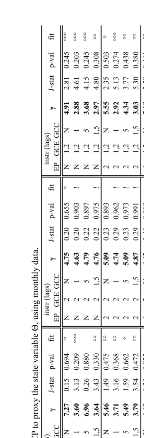
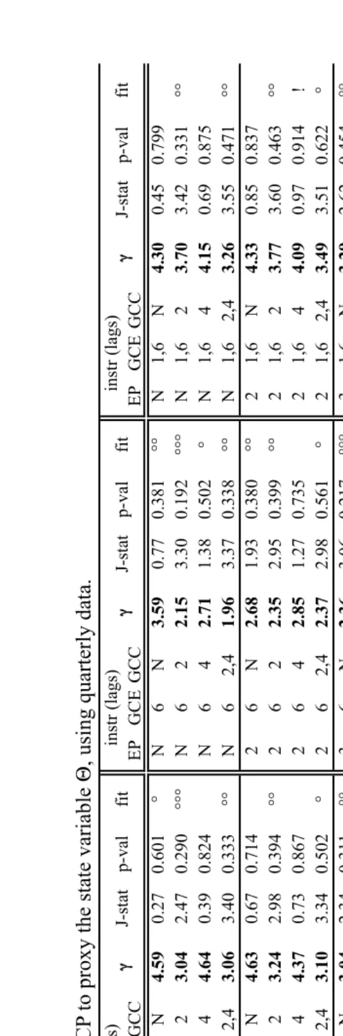
The fact that household forecasts about their future view of the economic performance are
…tting is illustrated in Tables 1-3, where we report the results obtained by regressing the current
value of CCP against its lagged value and the past realisation of CCE using monthly, quarterly
and yearly data, respectively. Under all speci…cations, the coe¢ cients of both regressors are
positive as expected and signi…cantly di¤erent from zero.17 The tables also report large R2, which suggests a very high goodness of …t. Adding other lags, or the past values of the overall
indicator, does not substantially increase the fraction of variance explained. Hence, we expect
CCP to produce analogous results as those produced by a potential composite index, in both our
quantitative and empirical exercises. In addition, the correlation between the present situation
component and the overall indicator, (which equals 0:94 in monthly and quarterly data, and 0:95 yearly,) suggests that current CC may also be used as a proxy for t.
Note that, substituting CCP for the state variable in the interpretation of the Euler
equa-tion (4) discussed in the last subsecequa-tion, it follows that consumpequa-tion growth is stimulated when
con…dence is currently high, and weakened otherwise. This prediction is in line with
empiri-cal evidence. Acemoglu and Scott (1994), Bram and Ludvigson (1998) and Ludvigson (2004)
…nd that lagged consumer con…dence (positively) predicts current consumption growth, which
remains signi…cant after controlling for variables such as income or labour income. It should
1 6The overall index is a weighted average of the two components, where 40% is the weight associated to the value of CCP.
1 7
be stressed, however, that our interpretation of con…dence as an indicator of the state of the
economy does not rely on its observed predictive power over consumption growth. In fact, we
argue that it is the link between the current value of the expectations component and the future
value of the present situation component to in‡uence consumption decisions, by portraying the
household view about the prospective conditions of the economy.
In this perspective, the link between con…dence and consumption growth would merely re‡ect
a by-product of household choice resulting from the twofold in‡uence exerted by the expected
performance of the economy (through the equity premia on the one hand, and satisfaction of
the consumption experience on the other). In particular: (i) the positive correlation between
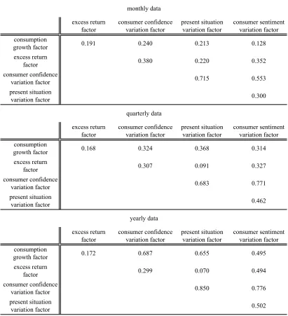
consumption growth and the excess return (from Table 5: between0:17 and0:19) suggests that …nancial incentives are a fundamental driver of the household decision; while (ii) the positive
correlation between the excess return and the variation in the value of the Consumer Con…dence
Index (from Table 5: from0:3to0:38) points towards a positive link between …nancial incentives and changes in the household perception of the state of the economy.
Finally, notice that the index developed by the University of Michigan, though unsuitable
given our interpretation of the state variable, may still be used as an alternative proxy for the
performance of the economy by virtue of its strong correlation with the Consumer Con…dence
Index (0:83 in monthly data, 0:81 both quarterly and yearly). For robustness, we include the Consumer Sentiment Index among the proxies used to capture the state of the economy. To
summarise, in our quantitative exercises illustrated in the next section, we use in turn the
Consumer Con…dence Index (CC), its present situation component (CCP), and the Consumer
Sentiment Index (CS) as proxies for the state variable (and hence as an indirect measure for
households’satisfaction of their consumption experience).
4
Quantitative results
In our consumption-based asset pricing model, a new element, measured by the ratio of the
values taken by the state variable at two successive dates, appears in the stochastic discount
factor in (4). Section 2 has shown that expected future high values of the state variable induce
individuals to raise current (relative to future) consumption in order to smooth the value of
utility at di¤erent dates, thereby in‡uencing their intertemporal choice. The e¤ects of this
in‡uence are assessed quantitatively by exploring whether they help in resolving one of the most
famous drawbacks of the asset pricing theory, namely the equity premium puzzle.
The equity premium puzzle is an issue that arises empirically when the representative agent
paradigm is used to relate asset prices to investors’saving decisions. This problem, …rst described
by Mehra and Prescott (1985), originates from observing that the real return on equities have
years. The puzzle arises because consumption growth is stable, its correlation with the equity
returns is moderate, so the resulting covariance is too low to explain the equity premium, unless
the relative risk aversion (RRA) coe¢ cient is implausibly high. Household preferences, speci…ed
by a standard constant RRA utility function, are made consistent with such a large equity
premium only if the coe¢ cient of relative risk aversion is at least as large as twenty.18 In contrast, empirical works that have undertaken systematic investigations of cross-sectional data
on individual’s asset holdings to assess the nature of its utility function, pioneered by Blume
and Friend (1975), …nd that the RRA coe¢ cient is estimated to be just in excess of two.19 The di¤erence between the estimated and the required value of the relative risk aversion gives a
measure of the puzzle magnitude.
Predictions are tested by adopting two di¤erent approaches. First, following Mehra and
Prescott (1985), we propose a calibration of the model. By log-linearising the Euler equation
(4), we derive the relative risk aversion coe¢ cient implied by the U.S. data (described below) in
the last four and a half decades, and compare its value to that obtained by microeconometric
estimations. Second, in order to check the robustness of our …ndings, following Favero (2001)
we also implement a GMM estimation. After describing the dataset, we present the results of
these two exercises in turn.
Dataset
The Consumer Con…dence Index series, provided by the Conference Board, is available only for
four and a half decades. Hence, working only with the Mehra-Prescott dataset is not ideal to
test our predictions, as a yearly dataset may leave too few observations to obtain robust results.
The dataset is then reconstructed, exploiting the fact that con…dence indicators are provided
on a monthly basis. In particular, we use three di¤erent frequencies to perform our quantitative
exercises: monthly, quarterly and yearly.
We begin our description of the dataset with the entries for the proxies for the state variable.
Exploiting the fact that the Consumer Con…dence Index is released every two months since
February 1967, the quarterly and yearly dataset contain 183 and 45 observations, respectively.
The monthly dataset entries are instead restricted to the period when the indicator was released
on a monthly basis (since June 1977), yielding 427 observations. The same …gures apply to the
present situation component of the Index. Regarding the University of Michigan’s Consumer
Sentiment Index, the monthly dataset contains 420 observations, since the index is released
1 8The constant RRA utility function is typically employed in most macroeconomic frameworks to represent the representative agent’s preferences. In more recent contributions that make use of such a paradigm, the magnitude of the RRA coe¢ cient is even higher, in some cases up to 70.
1 9
at such a frequency since January 1978. Previously, this indicator was released every quarter
since November 1959, thus the quarterly dataset features 213 observations. Furthermore, the
Consumer Sentiment Index was released three times a year since 1953, leading to 60 entries in
the yearly dataset.
The rest of the variables have longer time series. Financial data are available since November
1952, featuring 722 (240, 61) observations in the monthly (quarterly, yearly) dataset. The
equity returns are derived from the price and dividend time series of the Standard & Poor’s 500
composite index. As a series for the bond returns, we use the monthly data of annual based
nominal yield on three-month U.S. government treasury bills. Since the rates are reported using
the bank discount convention, we get the non annualised monthly return by using the appropriate
conversion formula.20 Then, the nominal returns are converted in real terms by using the price index provided by the Bureau of Economic Analysis of the U.S. Department of Commerce. This
index is provided by the same institution as the consumption data (the latter is available since
January 1959, covering 648, 215, and 53 entries in the monthly, quarterly, and yearly datasets,
respectively). These in turn correspond to the sum of two series on real personal consumption:
expenditures on services and expenditures on nondurables.
To summarise, the datasets used for the quantitative exercises that exclude the state variable
contain a common sample of 648 monthly, 215 quarterly, and 53 yearly observations. The
datasets using the Consumer Con…dence Index, or its present situation component, as a proxy
for the state variables feature a common sample of 427 monthly, 183 quarterly, and 45 yearly
observations. Finally, the datasets using the Consumer Sentiment Index as a proxy for the state
variables feature a common sample of 420 monthly, 213 quarterly, and 60 yearly observations.
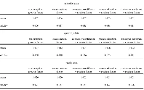
Tables 4 and 5 report the relevant descriptive statistics and correlations, respectively.
Calibration
We are now able to evaluate quantitatively the predictions of the Euler equation (4) by
calibrat-ing the model on observable U.S. data. Under certain assumptions, we …nd the followcalibrat-ing exact
log-linear expression for the terms in brackets of that equation:21
Etrat+1 rbt+1 = r[ rx x (1 ) r# #]: (5)
whererat+1 ln (1 +rA;t+1) and rbt+1 ln (1 +rB;t+1) represent the (geometric) rates of return on equities and bonds, respectively; subscriptsx and#refer toxt+1 = ln (Xt+1=Xt)and #t+1 = ln ( t+1= t), which denote the growth rates of consumption and average quality of consumption, respectively; gives a measure of the RRA coe¢ cient; i stands for the standard deviation of
2 0
See,e.g., Mayle (1993). 2 1
the variable i=fr; x; #g; ii0 is the correlation coe¢ cient between the variablesi; i0 =fr; x; #g, withi6=i0.
It is easy to make a comparison between this expression and the equation calibrated by
Mehra and Prescott (1985), given by:
Etrat+1 rbt+1 = rx r x: (6)
Equation (6) does not include the second term in brackets on the right-hand side of (5). Note
that, by de…nition, # >0 and >1. The e¤ect of this additional term thus depends on the sign of the correlation between equity premium and the variation in the proxy for the state
variable. The required magnitude of the RRA coe¢ cient is expected to go up if r#<0, and to decrease otherwise. From Table 5, it is straightforward that all the proxies for the state variable
variation factor deliver a positive correlation with the excess return factor. Hence, we expect
the calibration of (5) to produce a lower value for the RRA coe¢ cient than that resulting from
calibration of (6).
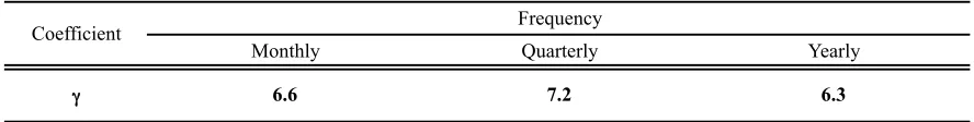
Table 6 reports the calibrations of the RRA coe¢ cient obtained with reference to (6) on
monthly, quarterly and yearly data. Under all speci…cations, the “standard” model implies a
value of RRA coe¢ cient well above80. Tables 7-9 report the calibration obtained with reference
to (5) on the same frequencies as above, using data on the overall Consumer Con…dence Index
(CC), on its present situation component (CCP), and on the Consumer Sentiment Index (CS),
respectively, as proxies for the state variable . According to our model, the calibrated value
for the RRA coe¢ cient ranges from4:2to10:5. Our calibration strongly suggests that the Euler equation, augmented using con…dence indicators as proxies for the e¤ect of the consumption
experience satisfaction on household decisions, reduces the required magnitude of the RRA
coe¢ cient at least by a factor of 8(and up to a factor of 23). As a result, our calibrated values
for the RRA coe¢ cient are clearly much closer to the interval 2 [2;4], where the economic literature estimates the true value of that coe¢ cient actually lies, than those derived from the
benchmark model.
Finally, it is worth noting that the value of the RRA coe¢ cient obtained by calibrating (5)
using data on the Consumer Con…dence Index is smaller than those obtained by using data on
its present situation component or the Consumer Sentiment Index. This is due to the fact that
variations in CC correlate much more with equity returns than variations in CCP, and are much
more volatile than changes in CS.
GMM estimation
For robustness, a number of estimations are implemented, based on a non-linear instrumental
optimization and rational expectations (IOREH), the only relevant variables in predicting
con-sumption at datet+ 1given the information at date tare consumption and the state variables at datet. Denoting the Euler equation (4) generically asf(yt+1; ), we have
Et[f(yt+1; )] = 0; Et[f(yt+1; )zt] = 0;
where yt+1 is the vector of observed variables of interest at date t+ 1, is the vector of parameters to be estimated, andztis a vector containing any economic variables observable at
date t. These two expressions essentially imply that the conditional expectation for date t+ 1 taken at datetof the term in brackets is in fact zero. Moreover, f(yt+1; )is orthogonal to any variable other than consumption and the state variables included in the agent’s information set
at datet. Notice that the Euler equation does not have any implication for the contemporaneous relation between consumption and other economic variables.
Euler equations from intertemporal optimization and rational expectations usually delivers
a potentially in…nite number of valid instruments. In this application, any lagged variable is
a valid instrument under the null that the IOREH model is a data generating process. The
parameters can be therefore estimated by using orthogonality conditions based on the following
set of instruments:
constant, t+1 t
; Xt+1 Xt
; 1 +rA;t+1 1 +rB;t+1
;
where we have chosen various combination of lags such that = [1;6]when dealing with monthly data, = [1;4]quarterly, and = [1;2]yearly.22
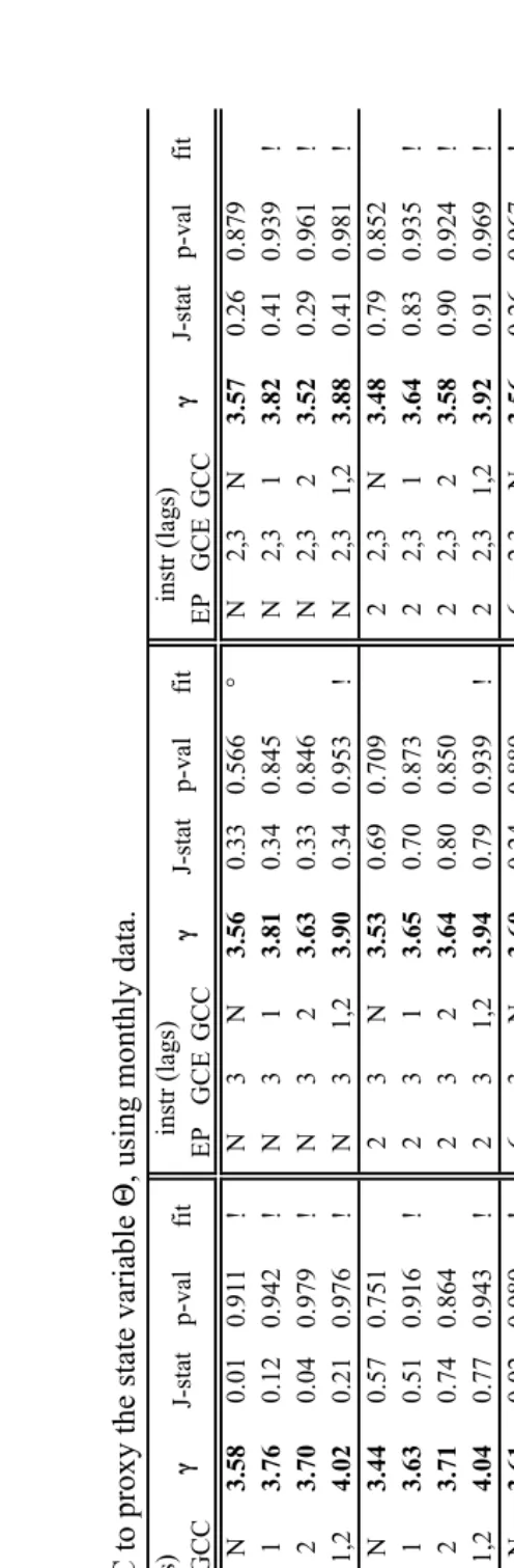
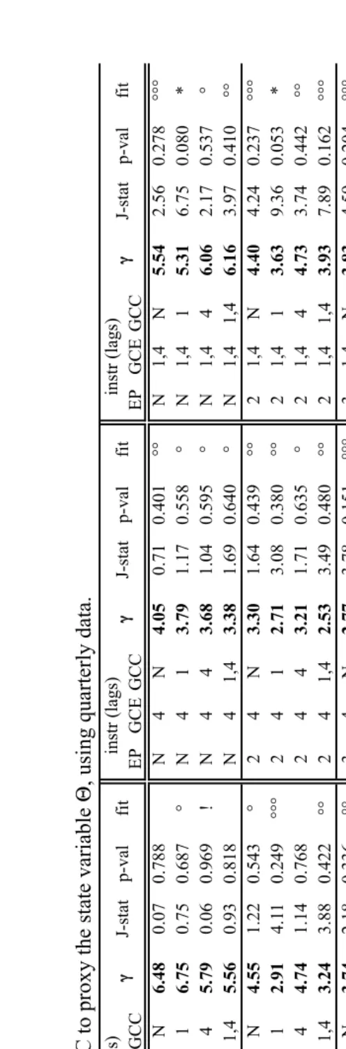
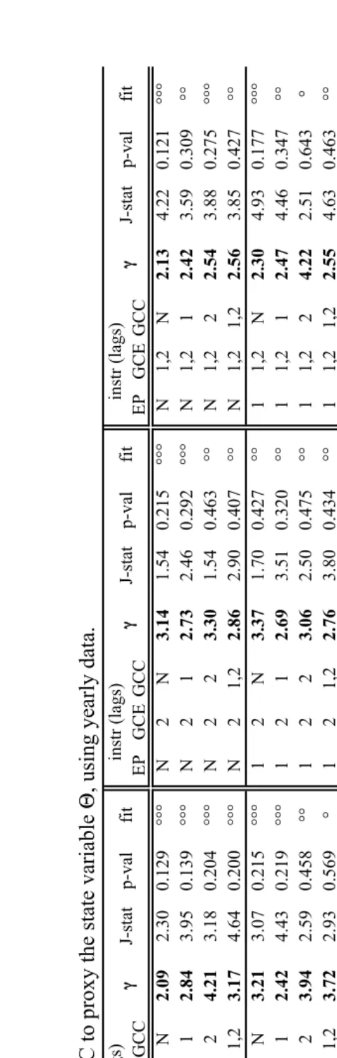
The quantitative results of the GMM estimations are once again based on the dataset
de-scribed above. The estimates obviously di¤er in the choice of the proxy used for the state
variable, that is the overall consumer con…dence index (CC), its present situation component
(CCP), and the consumer sentiment index (CS). Estimation of the Euler equation (4) is
imple-mented by using the appropriate routine in the E-Views software, using the HAC (Newey-West)
weighting matrix, with the Hannan-Quinn criterion for whitening lag speci…cation and the
An-drews’bandwidth method and the Tuckey-Hanning routine to implement the kernel, in order to
choose the appropriate lag truncation parameter.
The results are reported in Tables 10-21. Firstly, Tables 10-12 report the results obtained
by estimating equation (4) when considering t+1= t= 1; 8t2 N on monthly, quarterly, and yearly data respectively. Tables 13-21 report those obtained by calibrating the same equation
using data on con…dence indecators as proxies for t, again on the three frequencies respectively.
Regarding the standard model, although the estimates are qualitatively analogous to the results
2 2
obtained by calibration, the magnitudes of obtained here generally drop: the range is between
50 and 74 (calibrated: 95) on a monthly frequency, and between 28 and 68 (113) quarterly.23 In the literature, this result has often been regarded as suggestive of a greater signi…cance of
the higher moments of the joint distribution between consumption growth and excess returns
than typically believed. As such, together with the evidence linking con…dence and consumption
growth, it could appear to advocate for a role for con…dence in explaining habit formation in
consumption, or precautionary saving. However, the outlined ‘trend’ does not clearly appear
in the estimations reported in Tables 13-21: there, the range is 2:9 to 7:3 (4:2) on a monthly frequency, 0:3 to6:8 (4:8) quarterly, and 0:5 to 4:3 (6) yearly.24 In fact, all these estimations still lie in the range of values indicated by the literature as appropriate for the RRA coe¢ cient,
suggesting that con…dence may (though indirectly) re‡ect a more straightforward in‡uence on
household decisions.
5
Quality of consumption and the state of the economy
In Section 2, we have introduced a state variable into our consumption-based asset pricing model,
interpreting it as an indicator of the satisfaction in the household’s consumption experience. This
leaves us with the task of rationalising such an interpretation, particularly since it represents the
building block for the use of consumer con…dence as a proxy for the state variable. We perform
this task in three steps. First, we formalise a static framework with di¤erentiated consumption
goods, whose quality levels are subject to idiosyncratic shocks. Second, we show that this
framework can be easily embedded in the dynamic model, and relate the state variable to the
aggregate outcome of the deviations of the quality levels from their means. Third, we explore
the formal link between the state variable so obtained and the present situation component of
the Consumer Con…dence Index.
Static model
Exploiting the assumption that utility (1) is time-additive, we can think of household choice as
a two-stage problem. The second stage is the dynamic problem discussed in Section 2, whose
solution deliver the resource allocation over time, given the composition of the consumption
bundle. Here we discuss the …rst stage, which deals with the static choice of the optimal
consumption bundle composition, taking as given the resource allocation at the generic date
considered.
2 3We do not report the results obtained using yearly data, as the validity of instruments is rejected in all estimations.
2 4
Consider a unit continuum of horizontally di¤erentiated goods available for purchase,
rep-resented by the set Z R : z 2 [0;1]. Each good in the set Z is produced by a di¤erent …rm. Firms maximise pro…ts, and their productions consist of transforming labour services into
di¤erent …nal goods, according to sector-speci…c technologies.25 The production technology of each …rm z2 Z at a generic datet 2N is assumed to be concave in the amount of labour lz;t employed, that is:
yz;t= z;t(lz;t) ; (7)
where yz;t is …rm z output, and 2 (0;1) is a technological parameter. The terms z;t z2Z represent …rm-speci…c productivities. These are subject to idiosyncratic shocks (henceforth
referred to as technology shocks), which induce productivities to ‡uctuate around their (known)
mean values z z 2Z.
The novel feature of this framework is that technology shocks, denoted by f"z;tgz2Z, also in‡uence the quality dimension of production. We denote by fqz;tgz2Z the realised quality levels of the consumption goods, which also take values around their (known) means fqzgz2Z. Henceforth, we normalise the quality ladders to have a unit mean value, i.e., qz = 1, for all z2Z.26
The demand side of the economy is populated by a unit continuum of identical individuals,
each provided with one unit of labour services. Labour is homogeneous across individuals, so the
total labour force sums up to one (hence, the labour market clearing condition can be written
as RZlz;tdz = 1). Individuals derive utility by consuming a bundle of the goods available for purchase. The consumption indexCtmeasures one-period utility of consuming that bundle, and is de…ned by the constant elasticity of substitution (CES) function of Dixit and Stiglitz (1977)
type:
Ct= Z
Z
qz;t(xz;t) dz 1
; (8)
where 2(0;1) is a parameter governing the (limited) consumption elasticity of substitution among the di¤erent commodities,fxz;tgz2Zare the quantities consumed, andfqz;tgz2Zrepresent the quality levels of the goods consumed.27 Denoting by p
z;t > 0 the price for a consumption
2 5
To simplify matters, the goods set is invariant over time (hence innovation is ruled out), and all stock variables (physical capital, human capital, etc.) are normalised to one.
2 6Formally, each technology shock a¤ects …rmzproductivity according to the process
z;t ze
"z;t, and good z quality via qz;t e z"z;t, where the parametersf zgz2Z re‡ect the heterogenous impact of technology shock
across the di¤erentiated goods. The shocks have zero mean,i.e.,E("z;t) = 0for allz2Z, and variance-covariance
matrix such that static (across-goods) correlation is allowed, i.e.,cov("z0;t; "z00;t) 6= 0 for allz0; z00 2Z, but
serial correlation is prevented,i.e.,cov("z0;t0; "z00;t00) = 0for allz0; z002Zandt06=t00.
2 7
unit of good z, and by St the resources allocated to consumption at date t, the static budget
constraint reads: Z
Z
pz;txz;tdz St (9)
Both the representative household and all …rms solve the static problem after the current
state of nature is realised. That is, all agents are aware of the realisations of all types of shocks.
The representative household solves:
max fxz;tgz2Z
Ct= Z
Z
qz;t(xz;t) dz 1
;
subject to: Z
Z
pz;txz;tdz=St:
(10)
From the solution of problem (10), the following expression for the inverse demand for each good
z obtains:28
pz;t=qz;tPt(Ct)1 (xz;t) 1: (11)
The solution also implies that the maximised value of the consumption index (8) must equal
nominal spending, de‡ated by a suitable price de‡ator:
Ct= St Pt
; (12)
where Pt = Z
Z
(qz;t)11 (pz;t) 1 dz 1
represents the price index that must be used to
convert nominal variables in terms of the numeraire Ct.
Each …rm z2Zmaximises pro…ts by appropriately setting the optimal amount of labour to hire, taking household demand (11) as given. The production technology is given by (7). The
z-th …rm problem can be formally stated as follows:
z;t= max
lz;t qz;tPt(Ct) 1
z;t (lz;t) wntlz;t; (13)
where wtn is the (nominal) wage spent to hire one unit of labour services. From the solution of problem (13), considering the goods market clearing condition xz;t = yz;t, the following equilibrium allocation obtains:29
xz;t= ( t) (qz;t)1 z;t 1
1 ; (14)
where t
R
Z(qz;t)
1 1
z;t 1 dz. It is easy to notice that the response of the equilibrium
levels be determined exclusively by exogenous supply-side factors. 2 8
For the complete derivation of (11) and (12), see Appendix B. 2 9
allocation to technology shocks is positive: that is, a rise in the quality of the good reinforces
the e¤ect of an increase in productivity, implying a greater quantity exchanged.
Consumption and the state variable
Substituting (14) into (8), the consumption bundle can be rewritten as:
Ct= Z
Z
(qz;t)1 1
z;t 1 dz 1
(15)
In this form, the value of the consumption bundle captures all e¤ects arising from
technol-ogy shocks hitting …rm-speci…c productivities z;t z
2Z in (7) and good-speci…c quality levels
fqz;tgz2Z in (8). Once again, the relationship between the consumption bundle and each type of shock is positive. The value of the bundle is therefore the higher the greater the shocks to
quality (and productivity).
To compare the value of the consumption bundle in our model, where technology shocks
a¤ect the quality levels of the consumed goods, with the one in the benchmark model, where
shocks only in‡uence …rm productivities, we construct a baseline consumption index, denoted
byXt, by replacing the realised quality levels in (8) with their mean values,i.e.,qz;t= 1, for all z2Z:
Xt=
Z
Z z;t
1 dz 1
: (16)
The original consumption bundle Ct can be then written as:
Ct= tXt; (17)
where, using (8) and (16), and rearranging, t is formally given by:
t=
2 6 6 4 Z
Z (qz;t)
1 1
z;t 1 dz
Z
Z z;t
1 dz
3 7 7 5
1
: (18)
In the light of its structure, (18) can be interpreted as the weighted average quality of the
consumption bundle, with realised productivities as weights. Hence, average quality taccounts
for deviations from the mean values of quality levels in conjunction with those of technology,
net of the aggregate e¤ect of sole productivity shocks, which is captured by the consumption
bundle (16).30 3 0
One may argue that the stochastic processes governing quality and productivity observationlly display posi-tive trends. This fact, for simplicity unaccounted for by our stylised model, would in‡uence the behaviour of t
The interaction between quality levels and productivities a¤ects the average quality by
mag-nifying (if z;t >1) or reducing (if z;t <1), for each good z, the role of each realised quality levelqz;t. In particular, since the deviations of quality levels and productivities always “match”, then the larger the fraction of …rms hit by a positive shock, the higher the value of the average
quality of the consumption bundle. In fact,ceteris paribus, a positive technology shock increases
the value of z;t, (in…nitesimally) raising both the numerator and the denominator of (18). The
relative magnitude of these increments depends on the deviation of the quality level from its
mean: since the sign of this deviation is the same as for productivity, then the numerator rises
more than the denominator, and the resulting value of average quality is higher; the opposite
naturally occurs when the shock is negative. As a result, the larger the fraction of sectors where
shocks are positive, the greater the corresponding value of t, and the higher the value of the
consumption index Ct relative to the consumption index Xt.
In order to get an immediate grasp on the relationship between technology shocks and average
quality of consumption, consider for a moment the case of full symmetry, in which …rms have
identical production functions, are hit by a common shock, and produce goods whose quality
has identical responses to the common shock. Formally, this amount to assuming that z = ,
"z;t = "t, and z = , for all z 2 Z. Under this conditions, using the de…nitions of z;t and qz;t, and recalling that by de…nitionqz = 1for all z, the function capturing the average quality of consumption simpli…es to t =e( = )"t, from which it straightforwardly follows that tQ1 whenever "tQ0. Interpreting "t as the prevailing technology shock in the economy, this result implies a positive link between the overall state of the economy and the average quality of
consumption. In other words: (i) the utility of any given level of consumption, measured by
( tXt)1 , tends to be magni…ed by tin good times, and reduced in bad times; (ii) the marginal
utility of consumption, measured by(1 ) ( tXt) , has the opposite response, decreasing in good times and increasing in bad times, as we discussed after eq. (3).
State variable and consumer con…dence
From a theoretical perspective, Questions 1 and 2 may be translated into algebra, using the
equilibrium conditions just found, to obtain a formal representation of the CCP component. As
we discussed above, shocks to technology in‡uence the performance of the economy by enhancing
or reducing the ability of …rms to generate pro…ts and labour demand. In this mechanism, the
relative quality of the di¤erentiated goods also play a role, assigning more or less weight to the
realised productivity shocks in the di¤erent sectors.
The aggregate performance of the economy can be then assessed as follows. First, we compute
aggregate pro…ts t=Pt and wageswt in real terms, as predicted by the model presented in the
previous section. Then, we compare these …gures with those that would obtain by adopting a
model abstracting from technology shocks, i.e., =P andwrespectively. Notice that both asset and labour supplies are assumed to be …xed, and labour is inelastically supplied. As a result,
prices rather than allocations in these markets must be used to assess the economic performance.
Formally, the CCP indicator at date tis thus computed as follows:31
CCPt = wt
w + (1 ) t Pt=P
= 2 4 R
Z(qz;t)
1 1
z;t 1 dz
R
Z z 1 dz
3 5
1
(19)
where is the relative weight attached to real wages (if we followed the equal weight attached
to each question of the index, then we would simply have = 0:5).
Although the denominator presents the mean values z z2Z rather than the e¤ective real-isations f zgz2Z, the e¤ects of sectoral shocks on (19) are qualitatively analogous to those on the average quality of consumption (18). Compared to the hypothetical state of nature where
aggregation weights are deterministic, every variation in quality emphasizes (if the realised
tech-nology shock is positive) or dampens (if negative) the corresponding e¤ect of productivity. A
larger fraction of sectors where shocks are positive thus implies a value of CCPt greater than one, whereasCCPt<1 otherwise.
6
Concluding remarks
This paper has proposed a state variable augmented speci…cation of an otherwise standard asset
pricing model. An alternative version of the stochastic discount factor has been derived, which
crucially depends on the variations in the state variable. We have shown that the state variable
can be proxied by consumer con…dence indicators. The model has predicted that consumption
growth is inversely related to variations in consumer con…dence. This prediction, which is in line
with existing empirical evidence, has been assessed quantitatively by calibrating the relative risk
aversion (RRA) coe¢ cient to assess whether our setting reduces the empirical drawback known
as the equity premium puzzle. We have found that the model eliminates the puzzle. Our results
are robust to the estimation of the RRA coe¢ cient using the GMM methodology, to the use of
di¤erent data frequencies, of various indicators of con…dence, and to a number of instrument
speci…cations.
One of the most attractive features of this paper is perhaps the innovative representation
3 1
of sectoral shocks presented here, which allows for an intuitive connection between the state
variable and observed indicators of con…dence. There exists substantial evidence that
consump-tion growth and individuals’con…dence are positively correlated. Observing the data suggests
that there is evidence of high (low) growth rates of consumption when con…dence takes larger
(smaller) values. This stylised fact is in line with the predictions of our intertemporal Euler
equation. In conclusion, the model appears to provide a sensible theoretical explanation to the
empirical evidence relating individual’s con…dence to consumption growth.
The “preference shock” augmented setting can be easily exploited to address other asset
pricing issues, such as the evaluation of options and other derivatives, or investment. Some of
these issues are already the subject of ongoing research. Another …eld to which our framework
straightforwardly relates, notably for the fact that the state variable can also be seen as the
result of a price index decomposition, is monetary economics. In light of the result presented
here, it is arguably sensible to conjecture that individuals’con…dence may alter the transmission
mechanism of monetary policy, as predicted by using a standard sticky-price model.
The ‡exibility of the framework presented here allows it to be used in virtually every study
involving the derivation of a Euler equation, although only short-medium term models should
be considered. In the short-medium run, in fact, it is reasonable to consider that a fairly stable
state of nature characterizes each date. Longer time intervals, viewed as aggregations of short
periods, comprise several realised state. The successive states of nature that obtain in that
interval, by generating di¤erent sets of idiosyncratic shocks that typically end up o¤setting one
another, dampen the e¤ects of these shocks on individuals’ demand and …rms’ pricing, and
thereof on the equilibrium. If the number of consecutive states that obtain is large enough, then
such e¤ects eventually die away, possibly making long-term preference shock augmented studies
Appendices
A
Exact log-linear Euler equation
De…ne rh
t+1= ln (1 +rj;t+1), h=fa; bg andj =fA; Bg,xt+1 = ln (Xt+1=Xt)and#t+1 = ln ( t+1= t).
Assume that the vector of the log of the stochastic variables in (4) has a joint multinormal distribution:
z=
2 6 6 4
ra
x #
3 7 7
5 N
0 B B
@ =
2 6 6 4
r
x
# 3 7 7 5; =
2 6 6 4
2
r rx r#
rx 2x x# r# x# 2#
3 7 7 5
1 C C A
where i; 2i i=fr;x;#g are respectively mean and variance of variables fr
a; x; #
g, and
f ii0g
i;i0=fr;x;#g; i06=i measure the covariances among these variables. De…ning the vectors of the
ex-ponents in (4), suitably ordered, as 0a=h1 1
i
and 0b=h0 1
i
, the Euler equation (4) becomes:
Et[exp ( 0azt+1)] = exp rtb+1 Et[exp ( 0bzt+1)]
Recalling that the moment generating function for the Gaussian distribution is given by M( ) =
Et[exp ( 0z)] = exp ( 0 + 0 =2), and that the relevant moments are given by 0 = Pi i i and
0 =P
i 2i 2i + 2 P
i06=i i i0 ii0, after some algebra we obtain:
exp rbt+1 = exp r+ 2r=2 exp [ rx+ (1 ) r#]
Considering thatEt exp rat+1 = exp r+ 2r=2 , taking logarithms of both sides, using the de…nition
of correlation coe¢ cient, i.e. ii0 = ii0=( ii i0i0)1=2,i; i0 =fr; x; #g andi0 6=i; and rearranging, we get
(5).
B
Auxiliary derivations
Derivation of Equation (4). Replace (2) into (1) to obtain:
U = max
fjt+1gj=fA;Bg; t2N
E0
8 > < > :
X t2N
t ( t)1
h
wt+Pj=fA;Bg(1 +rj;t)jt jt+1
i1
1
9 > = > ;:
The …rst-order condition for the solution consists of the set of simultaneous equations:
@U
@At+1
= E0 n
( t)1 (Xt) + (1 +rA;t+1) ( t+1)1 (Xt+1) o
= 0; 8t2N;
@U
@Bt+1
= E0 n
( t)1 (Xt) + (1 +rB;t+1) ( t+1)1 (Xt+1) o
Dividing both equations by( t)1 (Xt) , taking constants out of expectations, and rearranging:
E0
(
(1 +rA;t+1) t+1 t
1
Xt+1
Xt
)
= 1; (20)
E0
(
(1 +rB;t+1) t+1 t
1
Xt+1
Xt
)
= 1: (21)
Equating the left-hand sides of (20) and (21), simplifying and rearranging, (4) obtains.
Derivation of Equation (11).
The representative household chooses, by appropriately setting the quantityxz;tof consumption for each
good z 2 Z, the optimal composition of the commodity bundle Ct, taking the resources St devoted
to consumption as given. Since utility (8) is a monotonic function of consumption, the static budget constraint (9) holds with equality. The Lagrangian therefore reads:
Lt= max
fxz;tgz2Z
Z
Z
qz;t(xz;t) dz
1
+ t St Z
Z
pz;txz;tdz ;
where t is the Lagrange multiplier associated toLt. The …rst-order condition for the solution consists
of the set of simultaneous equations:
@Lt
@ t
= St Z
Z
pz;txz;tdz= 0;
@Lt
@xz;t
= Z
Z
qv;t(xv;t) dv
1 1
qz;t(xz;t) 1 tpz;t= 0; 8z2Z: (22)
Consider the …rst-order condition (22) for a generic commodity z. Raising both sides to the power
(1 ) 1, integrating across varieties, and rearranging:
Z
Z
qv;t(xv;t) dv
1Z
Z
qz;t(xz;t) dz= ( t) 1
Z
Z (qz;t)
1 1 (p
z;t) 1 dz:
After some basic algebra, de…ning the Lagrange multiplier tas the reciprocal of the price de‡ator yields:
Pt=
Z
Z (qz;t)
1 1 (p
z;t) 1 dz
1
(23)
Raise both sides of the …rst order condition (22) to the power(1 ) 1 and rearrange to get:
xz;t= (qz;t)
1 1 (
tpz;t)
1 1
Z
Z
qv;t(xv;t) dv
1
Using (8), and (23), after some basic algebra, the demand for each commodity z 2Zcan be expressed
by:
xz;t= (qz;t)
1 1 pz;t
Pt
1 1
Inverting (24) to isolatepz;t, (11) obtains.
Derivation of Equation (12).
Multiply both sides of the …rst-order condition (22) forxz;t, integrate across varieties, and rearrange to
have:
Z
Z
qv;t(xv;t) dv
1
= t Z
Z
pz;txz;tdz
Using (8) and (11), (12) obtains.
Derivation of Equation (14).
Disregarding the e¤ect of each atomless …rm’s decision on economy’s aggregates, di¤erentiating (13) with
respect oflz;t and equating the resulting expression to zero yields:
qz;tPt(Ct)1 z;t (lz;t) 1 wtn= 0:
the …rst order condition for the solution of problem (13) thus reads:
wnt = qz;t z;t Pt(Ct)1 (lz;t) 1: (25)
Isolatinglz;t:
lz;t= (qz;t)
1 1
z;t 1 h
Pt(Ct)1
i 1 1
(wnt) 11 ; (26)
integrating across varieties:
Z
Z
lz;tdz=
Z
Z (qz;t)
1 1
z;t 1 dz h
Pt(Ct)1
i 1 1
(wtn) 11 = 1;
and isolatingwtyields:
wtn= ( t)1 Pt(Ct)1 ; (27)
where t
R Z( z)
1 1
z;t 1 dz. Nesting (27) back in (26), after some algebra:
lz;t = (qz;t)
1 1
z;t 1 h
Pt(Ct)1
i 1 1
( t)1 Pt(Xtx) 1
1 1
= (qz;t)
1 1
z;t 1 ( t) 1
giveslabour servicesemployed by …rm z:
lz;t=
(qz;t)
1 1
z;t 1 R
Z(qv;t)
1 1
v;t 1 dv
(28)
Replacing (28) in (7), and considering the market clearing conditionxz;t=yz;t, the equilibrium allocation
Derivation of Equation (15).
Raising both sides of (14) to the power and multiplying byqz;t:
qz;t xz;t = ( t) (qz;t)
1 1
z;t 1
Integrating across varieties, raising both sides to the power1= , using (8) and the de…nition of t:
Ct =
Z
Z
qz;t xz;t dz
1
= ( t) Z
Z (qz;t)
1 1
z;t 1 dz
1
= h( t) t i1
we obtain the equilibrium value of aggregate consumption (15).
Derivation of Equation (19).
From (27), using (15), the equilibrium wage obtains:
wnt = (Ct) Pt(Ct)
1
= PtCt
= Pt Z
Z (qz;t)
1 1
z;t 1 dz
1
(29)
Hence wages in real terms are:
wt
wn
t
Pt
= Z
Z (qz;t)
1 1
z;t 1 dz
1
(30)
From (11), using (14) and the de…nition of t, the equilibrium price obtains:
pz;t = (qz;t)
1 1
z;t
1 1 P
t(Ct)
1 1
= (qz;t)
1 1
z;t
1 1
Z
Z (qz;t)
1 1
z;t 1 dz
1
Pt: (31)
From the de…nition of pro…ts, i.e. z;t = pz;txz;t wtnlz;t, using (14), (28), (29) and (31), after some
algebra:
z;t = (qz;t)
1 1
z;t
1 1 P
t(Ct)
1 1 (q
z;t)1 z;t
1 1 (C
t) 1 (Ct) Pt(Ct)
1
PtCt(qz;t)
1 1
z;t 1 (Ct) 1 = (qz;t)
1 1
z;t 1 Pt(Ct)
1 a
1 (q
z;t)
1 1
z;t 1 Pt(Ct)
1 a
1
pro…ts are:
z;t = (1 ) (qz;t)
1 1
z;t 1 Pt(Ct)
1 a
1
= (1 ) (qz;t)
1 1
z;t 1 Z
Z (qz;t)
1 1
z;t 1 dz
1 a
Integrating across varieties, and rearranging:
t
Pt
= 1
Pt
Z
Z
z;tdz= (1 ) Z
Z (qz;t)
1 1
z;t 1 dz
1+1 a
aggregate pro…ts in real terms obtain:
t
Pt
= (1 ) Z
Z (qz;t)
1 1
z;t 1 dz
1
(33)
Using (30) and (33) as a base to computew and =P, and then into the expression CSt= (wt=w) +
References
Abel, A. B.(1990): “Asset Prices under Habit Formation and Catching Up with the Joneses,”American
Economic Review, 80(2), 38–42.
Acemoglu, D., and A. Scott(1994): “Consumer Con…dence and Rational Expectations: Are Agents’
Beliefs Consistent with the Theory?,”Economic Journal, 104(422), 1–19.
Aschauer, D. A.(1985): “Fiscal Policy and Aggregate Demand,”American Economic Review, 75(1),
117–27.
Atkeson, A., and J. Lucas, Robert E(1992): “On E¢ cient Distribution with Private Information,”
Review of Economic Studies, 59(3), 427–53.
Becker, G. S., and K. M. Murphy (1988): “A Theory of Rational Addiction,”The Journal of
Political Economy, pp. 675–700.
Bencivenga, V. R. (1992): “An Econometric Study of Hours and Output Variation with Preference
Shocks,”International Economic Review, 33(2), 449–71.
Blume, M., and I. Friend(1975): “The Asset Structure of Individual Portfolios with Some Implications
for Utility Functions,”Journal of Finance, 30, 585–604.
Boldrin, M., L. J. Christiano, and J. D. M. Fisher(1997): “Habit Persistence and Asset Returns
in an Exchange Economy,”Macroeconomic Dynamics, 1(2), 312–32.
Boldrin, M., L. J. Christiano, and J. D. M. Fisher (2001): “Habit Persistence, Asset Returns,
and the Business Cycle,”American Economic Review, 91(1), 149–166.
Bram, J., and S. Ludvigson (1998): “Does Consumer Con…dence Forecast Household Expenditure?
A Sentiment Index Horse Race,”Economic Policy Review, 4(2), 59–78.
Busato, F. (2004): “Relative Demand Shocks,” Department of Economics, Working Papers 2004-11,
Department of Economics, University of Aarhus.
Campbell, J. Y., and J. Cochrane(1999): “By Force of Habit: A Consumption-Based Explanation
of Aggregate Stock Market Behavior,”Journal of Political Economy, 107(2), 205–251.
Carroll, C. D., J. C. Fuhrer, and D. W. Wilcox (1994): “Does Consumer Sentiment Forecast
Household Spending? If So, Why?,”American Economic Review, 84(5), 1397–1408.
Cecchetti, S., P. Lam, and N. Mark (2000): “Asset Pricing with Distorted Beliefs: Are Equity
Returns Too Good to Be True?,”American Economic Review, 90, 787–805.
Cochrane, J. H. (1989): “The Sensitivity of Tests of the Intertemporal Allocation of Consumption to
Near-Rational Alternatives,”American Economic Review, 79(3), 319–37.
Constantinides, G. M. (1990): “Habit Formation: A Resolution of the Equity Premium Puzzle,”
Journal of Political Economy, 98(3), 519–543.
Crozet, M., K. Head, and T. Mayer(2012): “Quality Sorting and Trade: Firm-level Evidence for