Practical Application of Fast Disk Analysis for Selective Data Acquisition

University of New Orleans

University of New Orleans

ScholarWorks@UNO

ScholarWorks@UNO

University of New Orleans Theses and

Dissertations

Dissertations and Theses

Summer 8-11-2016

Practical Application of Fast Disk Analysis for Selective Data

Practical Application of Fast Disk Analysis for Selective Data

Acquisition

Acquisition

sergey gorbov

University of New Orleans, New Orleans, [email protected]

Follow this and additional works at: https://scholarworks.uno.edu/td

Part of the Information Security Commons, and the Other Computer Sciences Commons

Recommended Citation

Recommended Citation

gorbov, sergey, "Practical Application of Fast Disk Analysis for Selective Data Acquisition" (2016). University of New Orleans Theses and Dissertations. 2230.

https://scholarworks.uno.edu/td/2230

This Thesis-Restricted is protected by copyright and/or related rights. It has been brought to you by

ScholarWorks@UNO with permission from the rights-holder(s). You are free to use this Thesis-Restricted in any way that is permitted by the copyright and related rights legislation that applies to your use. For other uses you need to obtain permission from the rights-holder(s) directly, unless additional rights are indicated by a Creative Commons license in the record and/or on the work itself.

Practical Application of Fast Disk Analysis for Selective Data Acquisition

A Thesis

Submitted to the Graduate Faculty of the

University of New Orleans

in partial fulfillment of the

requirements for the degree of

Master of Science

in

Computer Science

Information Assurance

by

Sergey Gorbov

University of New Orleans

ii

Abstract

Using a forensic imager to produce a copy of the storage is a common practice. Due to the large volumes of the modern disks, the imaging may impose severe time overhead which ultimately delays the investigation process. We proposed automated disk analysis techniques that precisely identify regions on the disk that contain data. We also developed a high performance imager that produces AFFv3 images at rates exceeding 300MB/s. Using multiple disk analysis strategies we can analyze a disk within a few minutes and yet reduce the imaging time of by many hours. Partial AFFv3 images produced by our imager can be analyzed by existing digital forensics tools, which makes our approach to be easily incorporated into the workflow of practicing forensics investigators. The

proposed approach renders feasible in the forensic environments where the time is critical constraint, as it provides significant performance boost, which facilitates faster investigation turnaround times and reduces case backlogs.

Keywords

iii

Table of Contents

Abstract ... ii

Keywords ... ii

Table of Contents ... iii

List of Figures ... iv

List of Tables ... v

Nomenclature and Abbreviations ... vi

Chapter 1 ... 1

Introduction ... 1

Related Work ... 2

Chapter 2 ... 3

Background ... 3

Target Filesystems ... 3

Disk Representation and Partial Image... 3

Logical Representation ... 4

Chunk Subsets... 5

Chapter 3 ... 7

Methodology ... 7

Disk Pre-Processing ... 7

Filesystem Processing ... 8

Analysis Strategies ... 9

Random Sampling in Bitmap Walking ... 13

Experiments ... 20

Chapter 4 ... 25

Selective Imager ... 25

Chapter 5 ... 28

Conclusion ... 28

Limitations and Future Work ... 28

References ... 29

iv

List of Figures

Figure 2.1. A disk represented as a set of fixed size chunks. ... 3

Figure 2.2. A typical disk layout. ... 4

Figure 2.3. Left portion: data representation from the filesystem's perspective. Right portion: raw data representation. ... 6

Figure 3.1. Disk Pre-Processing abstract schema. ... 8

Figure 3.2. The layout of a 500GB disk with 4 NTFS filesystems. ... 12

Figure 3.3. The chunk map produced by the bitmap-based strategy for the 500GB disk with four valid filesystems. ... 12

Figure 3.4. The ground truth chunk map for the 500GB disk with four NTFS filesystems. ... 12

Figure 3.5. Description of bitmap walking procedure for allocation-based analysis. ... 13

Figure 3.6. Example when 𝐷𝑇𝑏𝑖𝑡𝑚𝑎𝑝 > 𝐷𝑇𝑟𝑒𝑓 ... 14

Figure 3.7. Example when 𝐷𝑇𝑟𝑒𝑓 > 𝐷𝑆 ... 14

Figure 3.8. Data density for a fixed data step size. ... 15

Figure 3.9. Example of a falling and a rising edges. ... 16

Figure 3.10. Probability of misclassification a data region as a zero region for different data density and data transaction size values. ... 18

Figure 3.11. The probability of failure of the chunk map post-processing. ... 18

Figure 3.12. The chunk map produced by the allocation-based strategy for a 500GB disk without valid filesystems on it. ... 20

Figure 3.13. The ground truth chunk map for a 500GB disk. Red chunks represent the data that are located within the large zero region. ... 20

Figure 3.14. The chunk map produced by the allocation-based strategy for 500GB disk with 4 valid filesystems. .... 23

Figure 3.15. The bitmap-based chunk map for 2TB disk with two valid NTFS filesystems ... 24

Figure 3.16. The ground truth chunk map for 2TB disk with two valid NTFS filesystems. ... 24

Figure 3.17. The allocation-based chunk map for 2TB disk with two valid NTFS filesystems. ... 24

Figure 4.3. The design of the selective imager. ... 26

v

List of Tables

Table 3.1. An overview of the filesystem analysis strategies and their attributes. ... 7

Table 3.2. Random sampling with a fixed sample size and different transaction sizes. ... 17

Table 3.3. Random sampling with a fixed amount of transactions for different transaction sizes. ... 17

Table 3.4. Results of the allocation-based analysis of 500GB disk without filesystems. ... 21

Table 3.5. Results of the allocation-based analysis of 500GB disk with 4 valid NTFS filesystems. ... 22

vi

Nomenclature and Abbreviations

chunk - an atomic data unit for disk representation

chunk map - an ordered sequence of chunks that represent a source disk

generic bitmap - the generic interface to the allocation management facility of a filesystem bitmap mask - the interface that converts a chunk map in to a bitmap

complete bitmap - overlapping of the generic bitmap and the bitmap mask bitmap walking - the procedure that implies traversing the complete bitmap CBW - Coarse Bitmap Walk

1

Chapter 1

Introduction

Almost all digital forensics investigations require evidence preservation. Depending on the nature of the evidence being examined, different techniques apply in order to effectively extract data. For example, in order to extract data from non-volatile storage devices such as hard disk drives, solid state drives, and flash drives, forensic investigators typically use a tool called an imager. There are plenty of imagers available, both open source as well as commercial ones. Imagers vary from the simplest tools that blindly replicate a source device into a raw image (e.g., the Unix dd tool[1]), to complex software kits, e.g. AccessData FTK[2], X-way[3], ADF Triage[4] that can perform disk analysis and preserve data in special space-efficient forensic formats. The ultimate objective for an imager is to produce an accurate forensic image as quickly as possible, as time is often the critical limiting factor in forensic investigations.

The trend of continuously increasing capacity for non-volatile storage devices has created a problem known in the digital forensics community as the volume challenge. Traditional approaches to imaging require a complete copy of a source storage device, which means that the source disk must be read in its entirety. The two main constraints that impose time overhead are the speed at which the source disk can be read and the speed at which a forensic image can being written onto a destination disk that will hold the copy of the data.

The write constraint can be relaxed by using data formatting, which reduces the amount data to be written onto the copy of the evidence. Modern forensic formats typically use data compression for reducing space of a resulting image, while also incorporating hashing to preserve the authenticity of evidence (e.g., the Advanced

Forensic Format[5][6]). However, both formatting features come at the expense additional CPU overhead. Even if a

source device is plugged into a fast interface, imaging speed can still be degraded due to inefficient algorithms used by the imaging tool.

The read constraint has widely been discussed in the digital forensics community, and current trends are directed towards the selective imaging. For example imaging a 10TB storage device at the speed of the SATA3 interface (6GBit/s or 600MB/s) would take approximately 5 hours, which is actually not bad. However in practice an average SATA3 disk's read speed will be limited at approximately 150MB/s, which means that, in the ideal case scenario when the disk does not contain errors, the imaging time extends from 5 to 20 hours. The situation with solid state drives is a bit better, as they provide read speeds of 300 - 500 MB/s, depending on vendor. Nevertheless, as solid state drives gain popularity, they too will increase substantially in size, and exacerbate the volume challenge. Thus selective imaging is meant to reduce the quantity of data that is required, while attempting to maximize the quality of the resulting image.

2

Related Work

Turner described the concepts of selective and intelligent imaging and discussed a number of options available when capturing data in selective manner[7]. He also proposed the data container called a Digital Evidence Bag (DEB), which is used to store objects selectively gleaned from multiple sources. The logical and structured approach of DEB maintains provenance and integrity of the evidence.

Whereas Turner applied selectiveness only at the file level, J. Stuttgen introduced a more generic concept, where any data that can be found on disk is considered as an object of potential interest and included in the imaging process[8]. However Stuttgen's scheme involves a human in the loop, which imposes additional time requirement for an investigator to pre-process the evidence. Furthermore, as storage sizes increase even further, a fully-automated solution is preferable.

Richard and Grier proposed a rapid imaging technique called sifting collectors[9] and they developed various sifting techniques to identify relevant data on disk. Using The Sleuth Kit's (TSK)[10] disk analysis capabilities, they

automatically identified sectors associated with files of potential forensic interest. The file filtering is handled by specifying profiles that are essentially collections of regular expressions that express which files are relevant and should be collected. Once the analysis phase is done, the intermediary data, called grainset, is passed to a collector that extracts designated data from source disk and stores it as a sifted Advanced Forensic Format v3(AFFv3) image.

Richard and Grier achieved up to x13 speed increases by sifting out irrelevant disk regions. The weak link in sifting collectors is that it performs the selectiveness only on the filesystem level. Because of this limitation, sifting collectors cannot identify the presence of data on a sub-filesystem level, e.g., volume slack space, unallocated space. Such analysis requires different approaches, e.g., sampling[11][12][13][14], which we use in the present work. Another major limitation of sifting collectors was poor performance of the imager. Richard and Grier used the AFFv3 library[6] in order to produce .AFF format images and this library performs reading, hashing,

compression and writing routines sequentially. Such inefficient resource utilization ultimately degraded the imager's performance in all aspects: the source I/O read time, the CPU overhead imposed by hashing and compression, and the destination I/O write time. While our approach also generates AFFv3 images, we have completely parallelized both the AFFv3 implementation as well as our own imaging components, which rely upon it, all without compromising the portability that AFFv3 offers.

3

Chapter 2

Background

This chapter discusses essential background concepts that underlie our efforts to develop a time efficient and accurate forensic imager.

Target Filesystems

Carrier described in detail the most widely used filesystems and volume systems in his book File System Forensic

Analysis[16]. So as not to reinvent the wheel, we used the open source TSK API[17] in order to evaluate disk layout

and run analysis on filesystems. TSK does not rely on the native OS filesystem drivers, which can easily be subverted by malware, but rather it analyzes the disk in a direct and non-intrusive fashion, which ensures data integrity. TSK has support for a wide variety of volume and filesystem types.

As of today, Microsoft Windows has the largest segment of the commodity operating systems market, and Windows systems must typically be installed on a New Technology Filesystem (NTFS). Thus we mainly consider Windows filesystems in our effort. The FATxx filesystem has been around for long time and is still in widespread use. We do not support FAT16 at all, as it is very limited in maximum partition size and it is easy to simply capture the entire filesystem. FAT32 remains useful as a cross-platform filesystem, so we support FAT32, even though maximum partition sizes are relatively modest. The Linux ext3/4 family of filesystems and Mac HFS+ are also widely used, but in this initial effort we do not currently fully support them, deferring such support for future work. Nevertheless, any filesystem that is recognized and supported by the TSK has limited support and still can be analyzed.

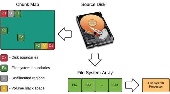
Disk Representation and Partial Image

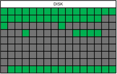
An operating system sees a storage device as a flat array of sectors, and a sector is an atomic unit for a storage device. A typical sector size is 512 bytes and while there are disks that support 4096 byte sectors, these typically have backward compatibility features that also support 512 byte sectors. Modern storage devices may consist of billions of sectors. For example, a disk volume of 6TB translates into 11,718,750,000 sectors. In our research effort, we will have to maintain state per storage unit to track which units are imaged, therefore, for the 6TB case, we would have to have an array of almost 12 billion elements to track sectors individually. This would be extremely inefficient, so for performance concerns we use a larger atomic unit called a chunk. A chunk is a fixed size data unit and can be: 2𝑥_{, where 𝑥 = [20, 29]. A disk representation using this strategy is shown in the Figure 2.1. The disk is}

represented as a set of chunks called chunk map.

- non-empty chunk

- empty chunk DISK

4

Any disk is considered to be a totally ordered set comprised of a finite numbers of fixed size chunks:

A chunk is considered empty if and only if all the bytes within the chunk are equal to zero, denoted 𝑧. Otherwise the chunk is considered to be non-empty, and is denoted 𝑧̅. Empty chunks never intersect non-empty chunks, i.e.,

∀𝑧, 𝑧 ∈ 𝑍, 𝑧 ∉ 𝑍 ̅ ; ∀𝑧̅, 𝑧̅ ∈ 𝑍,̅ 𝑧̅ ∉ 𝑍. In order to produce a full image 𝐼𝑓𝑢𝑙𝑙, all chunks must be included into the

final subset:

In order to produce a partial image 𝐼𝑝𝑎𝑟𝑡𝑖𝑎𝑙 , only selected chunks must be included: 𝐼𝑝𝑎𝑟𝑡𝑖𝑎𝑙 = 𝑓(𝐷), where 𝑓 is an

fast disk analysis function.

The ground truth partial image is the subset of all non-empty chunks: 𝐼𝑝𝑎𝑟𝑡𝑖𝑎𝑙𝐺𝑟𝑜𝑢𝑛𝑑𝑇𝑟𝑢𝑡ℎ = 𝑍̅. A filesystem may contain

legitimate files that are filled with zeroes and if, for example, a filesystem does not support spasrse files or a file is not set the attribute that turns on sparse storage feature, then such files might be also included into the ground truth partial image. In practice there is no way to produce an ideal ground truth image unless the entire disk is read. Our goal is to use fast disk analysis methods in order to compose the 𝐼𝑝𝑎𝑟𝑡𝑖𝑎𝑙, that is the closest

approximation to the partial ground truth image 𝐼𝑝𝑎𝑟𝑡𝑖𝑎𝑙𝐺𝑟𝑜𝑢𝑛𝑑𝑇𝑟𝑢𝑡ℎ. The difference Δ between the partial image and

partial ground truth image is expressed as a symmetric difference between 𝐼𝑝𝑎𝑟𝑡𝑖𝑎𝑙 and 𝐼𝑝𝑎𝑟𝑡𝑖𝑎𝑙𝐺𝑟𝑜𝑢𝑛𝑑𝑇𝑟𝑢𝑡ℎ:

The Δ subset sub-divides onto false negative and false positive subsets:

The false positives only impose additional overhead due to inclusion of empty chunks into the resulting image. The false negatives are undesired, as they break the completeness of the image. The overhead is evaluated as the following ratio:

Logical Representation

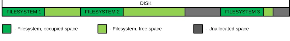
A disk can be considered as a complex infrastructure that accommodates multiple partitions and within each partition, a filesystem. In the scope of this research we only focus on the filesystem analysis. All problems related to integrity of volume systems, correct identification of partitions, and filesystem recognition are delegated to TSK, which has mature facilities for handling these issues. The Figure 2.2 shows the logical structure of a typical disk. The disk is logically split onto multiple partitions, which either contain a filesystem or a unallocated region.

DISK

FILESYSTEM 1 FILESYSTEM 2 FILESYSTEM 3

- Filesystem, occupied space - Filesystem, free space - Unallocated space

Figure 2.2. A typical disk layout.

A filesystem is a self-contained entity with numerous control structures and is aware of its own size. Each filesystem has a bookkeeping mechanism that allows for managing allocations and deallocations within the

𝐷 = 𝐶0∪ 𝐶1∪ … ∪ 𝐶𝑛 2.1

𝐼𝑓𝑢𝑙𝑙 = 𝑍 ∪ 𝑍̅ = 𝐷 2.2

𝐼𝑝𝑎𝑟𝑡𝑖𝑎𝑙∸ 𝐼𝑝𝑎𝑟𝑡𝑖𝑎𝑙𝐺𝑟𝑜𝑢𝑛𝑑𝑇𝑟𝑢𝑡ℎ= Δ 2.3

Δ = 𝐹𝑁 ∪ 𝐹𝑃 2.4

5

filesystem's storage space. A filesystem distinguishes only two regions, allocated (shown as green), and not allocated (shown as light-green). A filesystem uses a mechanism that keeps track of free space. The NTFS uses a bitmap that is a flat array of bits, each of which represents one cluster on the filesystem. If a bit in the bitmap is set then the associated with it cluster is allocated, otherwise the cluster is not allocated. FATxx systems use a similar approach but instead of a literal bitmap they use a file allocation table (FAT), which serves two purposes. First, each entry contains a reference to the next entry, such that walking the chain of entries in the FAT tracks file fragments. The second purpose is that it keeps track of allocations, i.e., if an entry has a non-zero value then the cluster associated with that entry is either used by some file, or is a bad cluster. The important issue is that regardless of the specific mechanism, filesystems know which regions are free and which are occupied.

The front end of a filesystem is the abstraction of file, directory, and an interface for interacting with these objects. There are a wide variety of filesystems in current use and while different filesystems may have completely

different internal mechanisms, they carry out many of the same functions. TSK abstracts away these differences between filesystems and allows for conducting filesystem analysis in a generic way.

The contents of a filesystem can be treated as the filesystem's critical metadata structures plus a set of files. Each file is defined by metadata and typically has associated with it a group of clusters. There are also special types of files, which may not have distinct clusters associated with them (e.g., very small files on the NTFS are stored within the $MFT entries). File attributes and parameters are maintained by a file metadata facility, e.g. $MFT on NTFS. Any file that is currently allocated and has valid metadata can be located and accessed. If a file has been deleted, then its metadata may be fully or partially destroyed. In this case the file is unrecoverable via the filesystem's facilities. An example of a filesystem that does not facilitate data recovery is the ext3/4, which explicitly destroys the inode blocks chains associated with a file upon deletion, making it impossible to retrieve the deleted file via the filesystem. However, there are filesystems that do facilitate data recovery, whether as an intentional design choice or otherwise. These do not completely destroy the metadata upon file deletion, which allows queries against the file metadata facility to reveal the data clusters associated with the deleted file. Nevertheless, even if the filesystem facilitates file recovery, there are cases when recovery fails. There are two required conditions for the recovery to succeed. First, the file metadata must be intact in order to correctly locate the clusters and recover the file content. Second, the clusters must not be overwritten by other data, otherwise the content will be not recoverable. The clusters no longer associated with active files typically linger in the filesystem until they are reused.

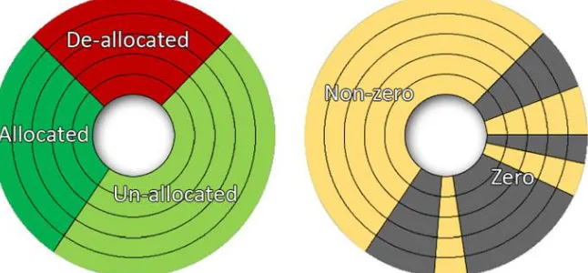
Thus, a typical filesystem's contents can be expressed as a union of the three data subsets:

An unallocated region(shaded regions) is considered any region that was not identified by TSK as a valid filesystem. Our approach allows for fast allocation pattern analysis within the disk, therefore each unallocated region can be pre-analyzed, and an appropriate decision can then be made accordingly.

Chunk Subsets

In the left portion of Error! Reference source not found., data is represented from the filesystem perspective. As in e xpression (2.6), there are three subsets that comprise the filesystem.

6

Figure 2.3. Left portion: data representation from the filesystem's perspective. Right portion: raw data representation.

The allocated subset describes critical filesystem structures that are required for a filesystem to properly function. The allocated subset also includes all currently allocated data that is available to user. Imaging only the allocated region is enough for a filesystem to operate normally. Therefore, the allocated subset has the highest priority in terms of forensic imaging, and must be included in the resulting image.

The deallocated subset describes data regions that were occupied by files in the past until they were deleted. Deleted files are often of forensic interest, as an adversary might delete some portions of available evidence either during a normal course of action or in a deliberate attempt to render data unrecoverable. Like the allocated subsets, deallocated subsets should be fully included in a forensic image.

Richard and Grier used the TSK API[17] for automated filesystem analysis and the approach they developed is able to efficiently identify allocated and deleted files and locate clusters associated with them. However, the scope of TSK does not extend to unallocated regions, which are also a part of the filesystem. Also, while a filesystem is aware of the limits of the unallocated regions, it is typically unaware of the content lingering in those regions. Unallocated regions may contain data that either has accumulated over time due to deletion of files and relocation of corresponsive metadata entries, or due to disk reformatting. Although the unallocated data within a filesystem is essentially a raw binary blob, it may contain important evidence or fragments of evidence. Therefore portions of an unallocated subset that contains data should be included into the resulting forensic image. In the right portion of Error! Reference source not found., there is an alternate view of the same, but expressed in zero and non-zero r egions. Denote the data part of unallocated region as 𝐹𝑆𝑢′ and an ideal resulting image would be:

7

Chapter 3

Methodology

From the discussion in the previous section, it is clear that in order create a partial forensic image that closely approximates the ground truth partial image, we must devise a disk analysis function 𝑓(𝐷) which will effectively identify chunks subsets 𝐹𝑆𝑎, 𝐹𝑆𝑑, and 𝐹𝑆𝑢′. The complete disk analysis can be split into disk pre-processing and

subsequent analysis of all of its partitions.

The processing of the contents of a partition may include more than one analysis strategy and specifically, we distinguish three fundamental strategies: file-based, bitmap-based, and allocation-based strategies. The three approaches differ in the principles they use to identify data regions. The file-based strategy utilizes the metadata facility on a filesystem in order to identify chunks that should be included into the final chunk subset. The bitmap-based strategy uses the allocation management facility on a filesystem in order to capture the allocated chunk subsets. The allocation-based strategy views the disk as raw data and applies statistical approaches in order to build up the unallocated subset 𝐹𝑆𝑢′ that contains data. The analysis strategies have four basic attributes: the

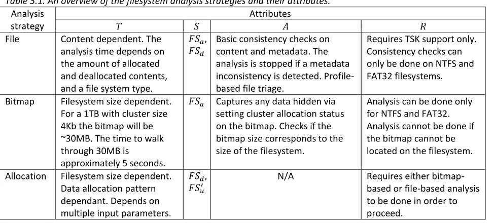
processing time 𝑇, the scope 𝑆, analysis capabilities 𝐴, and the prerequisites 𝑅, which define what is required in order to run the analysis routine. Table 3.1 briefly reviews the analysis strategies and their attributes. The analysis strategies are discussed in detail in the following sections.

Table 3.1. An overview of the filesystem analysis strategies and their attributes.

Analysis strategy

Attributes

𝑇 𝑆 𝐴 𝑅

File Content dependent. The analysis time depends on the amount of allocated and deallocated contents, and a file system type.

𝐹𝑆𝑎,

𝐹𝑆𝑑

Basic consistency checks on content and metadata. The analysis is stopped if a metadata inconsistency is detected. Profile-based file triage.

Requires TSK support only. Consistency checks can only be done on NTFS and FAT32 filesystems.

Bitmap Filesystem size dependent. For a 1TB with cluster size 4Kb the bitmap will be ~30MB. The time to walk through 30MB is

approximately 5 seconds.

𝐹𝑆𝑎 Captures any data hidden via

setting cluster allocation status on the bitmap. Checks if the bitmap size corresponds to the size of the filesystem.

Analysis can be done only for NTFS and FAT32. Analysis cannot be done if the bitmap cannot be located on the filesystem.

Allocation Filesystem size dependent. Data allocation pattern dependant. Depends on multiple input parameters.

𝐹𝑆𝑑,

𝐹𝑆𝑢′

N/A Requires either bitmap-based or file-bitmap-based analysis to be done in order to proceed.

Disk Pre-Processing

8

Figure 3.1. Disk Pre-Processing abstract schema.

One might be curious about why we are turning on chunks that designate boundaries for the disk and each volume. A typical disk normally starts with a Master Boot Record (MBR), but if the disk has a GPT structure then the first chunk will also include the primary GPT header, and the last chunk will capture the secondary GPT header. Even with the minimum chunk size that is equal only 1MB, these essential structures will be included into the resulting image.

A similar reason justifies capturing a volume's boundaries. Some volumes may contain a Volume Boot Record (VBR) structure, which is the first sector on the volume. Notably, however, a filesystem inside a volume might not be the same size as the volume. In this case there is slack space that can exist before the first byte of the filesystem and/or after the last byte of the filesystem. Some filesystems, e.g., NTFS, may use such this slack space to store a backup of the boot record. Therefore to ensure the integrity of the disk we add these corresponding chunks into the final chunk subset.

Any error during disk pre-processing will cause termination of further analysis, which will ultimately mean that the disk should not be analyzed using our methods because the disk metadata is corrupted. The analysis of corrupted disk may produce inaccurate results, which defeats the purpose of imaging. In this case the investigator is urged to produce a complete forensic image using traditional methods, if possible.

Filesystem Processing

After the disk pre-processing has completed, the resulting filesystem array is passed to the filesystem processor, where each filesystem object is analyzed individually. The filesystem processor is an abstract interface. For each filesystem the filesystem processor must be implemented individually. The objective of a filesystem processor is to check whether a filesystem meets sanity checks so it can be analyzed. If a filesystem passes consistency checks then it is approved for further analysis, otherwise it is rejected and added into the final chunk subset in its entirety.

9 Bitmap Interface

For each filesystem that successfully passes the consistency check we create a generic bitmap interface. A bitmap interface is an abstract entity that defines access operations for the allocation management facility of a filesystem. For NTFS, the generic bitmap interface simply provides access to the $Bitmap file. For FAT32, which does not have a literal bitmap, the generic bitmap interface provides on-the-fly translation of the FAT into a bitmap, e.g., each FAT entry is converted into one bit. Bitmaps are queried via a bitmap index, which represents one bitmap

transaction, spanning 64 sequential bits. Thus one bitmap transaction describes 64 clusters on a filesystem and

represents one data transaction. For a typical cluster size of 4096, the bitmap transaction translates into a data transaction of 262144 bytes. Thus larger cluster sizes result in larger data transaction sizes.

The bitmap interface provides optimizes the interaction with actual bitmaps using bitmap buffering, e.g., only a small size of a bitmap resides in the memory at any given time.

The main reason behind introducing the concept of a custom bitmap interface is that the bitmap is the central component for the bitmap-based and the allocation-based analysis strategies. The bitmap interface turns a static bitmap structure 𝐵, fetched from a filesystem into a dynamically updated bitmap by overlapping the actual bitmap with the bitmap mask 𝑀. The bitmap mask is a translation of chunk map region that corresponds to a filesystem being analyzed such that the complete bitmap 𝐵𝑐𝑜𝑚𝑝𝑙𝑒𝑡𝑒 is expressed as: 𝐵𝑐𝑜𝑚𝑝𝑙𝑒𝑡𝑒= 𝐵 ∪ 𝑀.

There is an edge case when a bitmap mask is used as a complete bitmap: 𝐵𝑐𝑜𝑚𝑝𝑙𝑒𝑡𝑒= 𝑀. For unsupported

filesystems the bitmap structure cannot be retrieved. If the filesystem is supported by TSK, then having conducted the file-based phase it is possible to produce a chunk map that may be used as a start point for the allocation-based analysis.

Analysis Strategies

File-based strategy

The files are located on the filesystem using their metadata information. Based on the byte offsets a file is expressed in terms of chunks and the file chunk subset is added to the final chunk map. This procedure is performed for all valid file metadata entries that TSK can discover on the filesystem.

During this phase there is a possibility of content or file metadata inconsistency. Content inconsistencies occur when allocated clusters are associated with more than one entry. A file metadata inconsistency occurs when a file's metadata indicates that its data is stored in a region of unallocated clusters or beyond the limits of the filesystem. Any inconsistency will stop further analysis and add the entire filesystem to the final chunk subset, since our tools do not currently differentiate between minor and major filesystem corruptions.

The file-based strategy is mainly used either for profile-based file triage or for non-supported filesystems in order to build up a bitmap mask based on the produced chunk map.

Profile-based File Triage

10 The profile supports three fundamental directives:

 :Files - defines the patterns for files. During the file search if a file matches at least one pattern the file

location is expressed in terms of chunks and added to the final chunk map.

 :Path - defines the patterns for paths. The mechanism is the same as in the case with files, but instead of

filenames, paths are evaluated according to the supplied patterns.

 :include - includes an existing profile into the current profile. This allows multiple profiles to be used in

conjunction.

The following section represents an example of a profile that targets pictures:

:Paths /Pictures /My Pictures /Pics /Photos

:Files \$

\.(png|gif|jpg|bmp|ppm|xbm|raw|tiff|tif|crw|cr2|nef)$

In order to supply desired paths and files we first supply a desired directive, e.g., :Paths or :Files. Any data supplied under the directive is considered related to that directive. A directive's scope ends if another directive is

encountered.

If we want to combine several profiles into one we use :include directive, as shown below:

:include "Email.profile" :include "Financial.profile" :include "Photography.profile"

:include "WindowsBrowserHistory.profile" :include "WindowsDataExfiltration.profile" :include "WindowsDocuments.profile" :include "WindowsLogs.profile" :include "WindowsRegistry.profile"

Files: \$

^SAM(\.log)?$ ^SECURITY(\.log)?$ ^SOFTWARE(\.log)?$ ^Default(\.log)?$ ^Userdiff(\.log)?$ ^Ntuser\.dat$ ^Usrclass\.dat$ ^Repair(\.log)?$ ^System(\.alt|\.log)$

11

The final chunk subset produced via profile-based file triage describes a filesystem in such a way that it can be mounted and analyzed as if it was cloned. In the resulting partial image the filesystem metadata will be preserved, so it will have an identical layout with the original filesystem. However an investigator will be able to access only those items that matched the search patterns—others will appear to be zero-filled.

This technique is useful if an investigator has a preliminary knowledge about the case, so he can quickly use the profile and extract only relevant data that may be several orders of magnitude smaller than the size of the entire disk. The complete procedure may take just a few minutes, compared to hours if traditional imaging were used.

The based file triage is a file-based analysis, and it inherits all the limitations related to it. Thus the profile-based file triage cannot be used if the filesystem is in an inconsistent state, e.g., has corrupted metadata. Another limitation is that if a filesystem is has a very large number of files, then in some cases it would be faster to image the entire filesystem. In particular, TSK processing time drastically increases as the amount of entries on a filesystem grows.

During the pre-processing stage, our tool summarizes some important information about each analyzed filesystem and provides this information to the investigator:

 The number of entries in the metadata management facility. For NTFS, this is information about how large the $MFT structure is. For filesystems like FAT32, we cannot provide this information, because there is no means to discover the number of files without searching for Directory Entries, which may be scattered all over the filesystem.

 The average read speed and approximate imaging time for a current filesystem. Thus prior to starting selective imaging, an investigator knows how long would it take to produce a complete image. In order to enable the read speed check feature the configuration must be adjusted, so the program knows the interface bandwidth. This is currently required due to caching issues.

Thus having basic information about the filesystem that is about to be passed for further analyses, an investigator can get a first impression of what to expect if the analysis proceeds. In any event, if the file-based analysis is predicted to take too long and is considered impractical, it can always be terminated, and other means used for further disk examination.

Bitmap-based strategy

The bitmap-based strategy captures all valid entries that are currently allocated on a filesystem. It is much faster than the file-based approach as it does not invoke TSK file searching routines, which may take a long time for filesystems with large number of files.

During the bitmap-based analysis, the complete bitmap is walked from start to ending bitmap index, sequentially processing each bitmap transaction. The entire complete bitmap can be expressed as a set of all the bitmap transactions, 𝐵𝑐𝑜𝑚𝑝𝑙𝑒𝑡𝑒= (𝑡𝑠𝑡𝑎𝑟𝑡, 𝑡𝑠𝑡𝑎𝑟𝑡+1, . . . , 𝑡𝑒𝑛𝑑).

Each chunk in the chunk map can be expressed as a subset of 𝑖 sequential bitmap transactions. If there is a chain of sequential bitmap transactions 𝐶 = (𝑡0, 𝑡1, … , 𝑡𝑖), ∀𝑗, 𝑗 ∈ [0, 𝑖], 𝑡𝑗= 0, then the chunk that corresponds to the

chain 𝐶 is said to be empty and is not added to the final chunk subset. Otherwise if at least one bitmap transaction is non-zero, then the entire chunk to which the transaction belongs is added to the final chunk subset.

12

500GB disk

327680000(167.8GB) 409600000(209.7GB) 81920000(41.9GB) 152571072(80.7GB)

Windows 8 2.5 years old Empty Random numbers Empty

Figure 3.2. The layout of a 500GB disk with 4 NTFS filesystems.

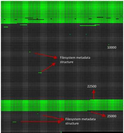
Comparing the Figure 3.3 with the Figure 3.4, we can see that they are slightly different. In particular, the bitmap capture is missing some deallocated data that is located within the first filesystem (the upper part). Analyzing the chunk maps, we can identify the limits of the filesystems, e.g., chunk 10000 is equivalent to sector 327680000, which corresponds to the end of the first filesystem and beginning of the second one. The second filesystem starts at chunk 10000 and ends at chunk 22500. It does not contain any data other than NTFS system files, therefore the region occupied by the second filesystem is almost completely filled with zeroes. The third filesystem contains a 40GB file filled with random numbers, therefore the entire range of chunks from 22500 to 25000 is filled with data. The last filesystem is analogous to the second filesystem and does not contain user data.

If a disk has valid filesystems then it is most likely that a large part will be captured during bitmap-based analysis. However it is also possible that a disk was reformatted. In this case the bitmap-based strategy will not be able to produce a sound chunk map, because the information about the allocations on the previous filesystem(s) has been destroyed. This raw data discovery is in the scope for the allocation-based routines.

Figure 3.3. The chunk map produced by the bitmap-based strategy for the 500GB disk with four valid filesystems.

Figure 3.4. The ground truth chunk map for the 500GB disk with four NTFS filesystems.

Allocation-based

Technically, the allocation-based strategy uses the same basis as the bitmap-based strategy. It is walking through the complete bitmap, but evaluates whether regions that are unallocated according to the bitmap may in fact contain non-zero data, corresponding to, e.g., deleted files. Such data composes the subset 𝐹𝑆𝑢′, that has been

defined earlier.

In order to identify a data subset 𝐹𝑆𝑢′ within an unallocated subset 𝐹𝑆𝑢 we use statistical analysis methods, namely

sampling[11]. The allocation-based analysis is split into two phases: the coarse bitmap walk (CBW) and the fine bitmap walk (FBW). The coarse bitmap walk is bitmap size dependent only, whereas the fine bitmap walk also

depends on the allocation patterns in a filesystem.

10000 Filesystem metadata

structure

Filesystem metadata structure

22500

25000 Filesystem metadata

structure

Filesystem metadata structure 10000

22500

13

Random Sampling in Bitmap Walking

In general, the idea behind sampling is to evaluate the characteristics of the entire disk without reading it in full, which would defeat the purpose of partial imaging. Therefore we read a small part of a disk, sufficient to identify the data subset 𝐹𝑆𝑢′ with an acceptable level of error and overhead. Garfinkel applied random sampling to identify

known artifacts and data presence, e.g., whether a disk was properly wiped[14].

The scope of allocation-based analysis is not concerned with file contents, but with the identification of regions that contain data. Simply applying sampling on the unallocated data subset 𝐹𝑆𝑢is not enough for identifying data

boundaries. Hence we need a robust way for accurate identification of data regions on a disk. We have employed the random sampling algorithm in bitmap walking procedures. The randomization part is necessary in order to ensure that there will be no easy way to predict where a sample is taken from.

Both phases of the allocation-based analysis have three common parameters that can specified by a user:

1. Maximum data step size, 𝐷𝑆𝑚𝑎𝑥 -- specifies the size of a disk to be sampled. After the data step is

established, it is randomly sampled with one data transaction. If the data transaction contains all zeros, then the entire step is assumed to be zeros. Otherwise the entire step is considered to be non-zero, expressed in terms of chunks, and then added to the chunk map. For CBW, this parameter is static and for the FBW this parameter is dynamic.

2. Reference data transaction size, 𝐷𝑇𝑟𝑒𝑓 -- specifies the data transaction size that is read from a data step.

This parameter remains fixed for both walking procedures throughout the analysis.

3. Join distance - specifies the minimum size in chunks for a zero region. All data gaps not larger than the join

distance are added to the resulting partial image.

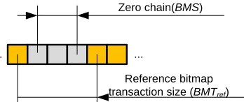
Figure 3.5 illustrates our bitmap walking procedure and the mapping between bitmap transactions (represented by yellow and light gray squares, where each square is a single bitmap transaction) and data regions (of size bitmap

data transaction size and represented by blue and dark gray squares). The notations related to the complete

bitmap facility are prefixed with "𝐵𝑀". The notations related to the data region facility are prefixed with "𝐷".

Figure 3.5. Description of bitmap walking procedure for allocation-based analysis.

Whereas the complete bitmap is addressed by a bitmap index 𝐵𝑀𝐼, the data region is addressed by actual data offsets on the disk. In order to convert a bitmap index into the actual disk offset the bitmap index must multiplied by the bitmap transaction data size, and the offset of the start of the filesystem must be added.

For a cluster size as 𝐶𝑆, the bitmap transaction data size that corresponds to one bitmap transaction is expressed

as: 𝐷𝑇𝑏𝑖𝑡𝑚𝑎𝑝 = 64 × 𝐶𝑆. The maximum data step size 𝐷𝑆𝑚𝑎𝑥 maps onto the complete bitmap where it is called the

14

In order to sample data on a given step, a chain of zero bitmap transactions must be accumulated. The quantity of sequential bitmap transactions is denoted as the current bitmap step 𝐵𝑀𝑆. For the zero chain 𝐶 = (𝑡1, 𝑡2, … , 𝑡𝑁),

where 𝐵𝑀𝑆 = 𝑁, there are two situations:

The scenario described by the expression 3.2 corresponds to the Figure 3.5. The chain of sequential zero bitmap transactions spans the bitmap indicesfrom 1 to 8. Due to encountering a non-zero bitmap transaction 𝑡9≠ 0, the

chain of sequential zero transactions breaks, having accumulated only 7 bitmap transactions that are equal zero. Thus, the resulting bitmap step size 𝐵𝑀𝑆 = 8 − 1 = 7, whereas the maximum bitmap step size 𝐵𝑀𝑆𝑚𝑎𝑥= 𝑛 − 1.

The scenario related to the expression 3.3 represents a case when the chain of sequential zero bitmap transactions has reached the maximum bitmap step size 𝐵𝑀𝑆𝑚𝑎𝑥 such that 𝐵𝑀𝑆 = 𝐵𝑀𝑆𝑚𝑎𝑥.

Denote the first bitmap transaction for the current step as 𝐵𝑀𝐼𝑠. In order to identify the location on the disk from

which to take a sample we need to calculate the data step start offset 𝐷𝐼𝑆that must correspond to 𝐵𝑀𝐼𝑠:

Since the current 𝐵𝑀𝑆 is known, the resulting data step size is calculated as:

Finally, the data transaction size 𝐷𝑇 for the given data step size 𝐷𝑆 is calculated as:

The data transaction 𝐷𝑇 may two edge cases:

1. The first case is depicted in the Figure 3.6, where 𝐷𝑇𝑟𝑒𝑓 < 𝐷𝑇𝑏𝑖𝑡𝑚𝑎𝑝. The resulting data transaction size in

this scenario will be always equal to 𝐷𝑇𝑟𝑒𝑓.

2. In the Figure 3.7 there is a case when 𝐵𝑀𝑆 corresponds to 𝐷𝑆 such that: 𝐷𝑇𝑟𝑒𝑓> 𝐷𝑆 ≥ 𝐷𝑇𝑏𝑖𝑡𝑚𝑎𝑝. In this

situation the resulting data transaction size will be equal to 𝐷𝑆.

Reference data transaction size (DTref)

... ...

Figure 3.6. Example when 𝐷𝑇𝑏𝑖𝑡𝑚𝑎𝑝 > 𝐷𝑇𝑟𝑒𝑓

... ...

Reference bitmap transaction size (BMTref)

Zero chain(BMS)

Figure 3.7. Example when 𝐷𝑇𝑟𝑒𝑓> 𝐷𝑆

𝐵𝑀𝑆𝑚𝑎𝑥=

𝐷𝑆𝑚𝑎𝑥

𝐷𝑇𝑏𝑖𝑡𝑚𝑎𝑝

3.1

𝑁 < 𝐵𝑀𝑆𝑚𝑎𝑥; ∀𝑘, 𝑘 ∈ [1, 𝑁], 𝑡𝑘= 0; 𝑡𝑁+1≠ 0 3.2

𝑁 = 𝐵𝑀𝑆𝑚𝑎𝑥; ∀𝑘, 𝑘 ∈ [1, 𝑁], 𝑡𝑘= 0 3.3

𝐷𝐼𝑆= 𝐷𝑇𝑏𝑖𝑡𝑚𝑎𝑝× 𝐵𝑀𝐼𝑠 3.4

𝐷𝑆 = 𝐵𝑀𝑆 × 𝐷𝑇𝑏𝑖𝑡𝑚𝑎𝑝 3.5

15 Sampling Parameters

Since the allocation-based analysis uses a statistical approach we have to evaluate the probability of

misclassification a data region as a zero region, 𝑃𝑚𝑖𝑠𝑠. The sampling accuracy for a given step 𝑖 depends on current

data step size 𝐷𝑆𝑖, the current data transaction size 𝐷𝑇𝑖, and the current data density, Φ𝑖, where Φ𝑖∈ [0, Φ𝑟𝑒𝑓],

and Φ𝑟𝑒𝑓 is the reference data density.

The reference data density is a data density of a region that contains data. Our imager will encounter a wide variety of data types and hence, allocation patterns. For example a compressed data typically has very high data density, whereas an uncompressed data may have much lower data density. The analysis of data types and their allocation patterns are beyond the scope of this research, and we are striving to choose parameters that work well in common scenarios Therefore we assume that the reference data density on a region that contains data is a fixed value Φ𝑟𝑒𝑓= 0.1. Thus any sector within a data region has the probability Φ𝑟𝑒𝑓 that it is not completely filled

with zeroes, e.g. at least one bit within the sector is set to 1.

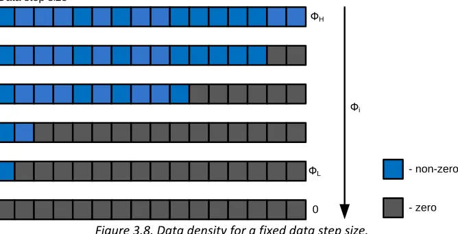
Throughout the analysis any given step 𝑖 may span the amount of non-zero data transactions that is smaller than

the data step size, thus forming data steps with different density Φ𝑖. In the Figure 3.8 there is an example of

possible data transaction layouts within a data step of a fixed size.

Фi ФH

ФL Data step size

0

- non-zero

- zero

Figure 3.8. Data density for a fixed data step size.

In the Figure 3.8 Φ𝐿 corresponds to a low data density, and Φ𝐻 represents a high data density. Each square

represents one data transaction. Each blue square is a non-zero data transaction and is assumed to have the data density Φ𝑟𝑒𝑓. Each dark-gray square is a zero data transaction and has data density 0.

The layout of data transaction within a given data step is not known and assumed to be random. Thus if we randomly read one data transaction from within a data step of size 𝐷𝑆𝑖 with 𝑛 non-zero data transactions, the

resulting data density is expressed as:

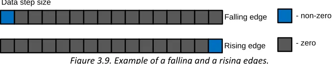
There are two edge cases for the data transaction layout. If there is a transition from a data region to a zero region then the layout within the data step forms the falling edge. If there is a transition from a zero region to a data region then the layout within the data step forms the rising edge. In the Figure 3.9 there are examples of rising and falling edges.

Φ𝑖= Φ𝑟𝑒𝑓

𝑛

16

Falling edge Data step size

Rising edge

- non-zero

- zero

Figure 3.9. Example of a falling and a rising edges.

In reality a data step size can include thousands of data transactions. Generally speaking, if data within a step is clustering at the beginning of the step, then the step represents the falling edge. If data within a step is clustering towards the end of the step, then the step represents the rising edge. The edges tend to have very low data density therefore they accuracy on them is lower than the accuracy on a solid data region.

Due to the fact that the CBW runs with a fixed data step size, it might not precisely capture the falling and rising edges. The edges are not dangerous within solid data regions as all the gaps that are not larger than the join distance will be smoothened during the chunk map post-processing. However the problem arises when a data region ends and the large zero region begins, or vice versa, a large zero region ends and data region begins.

The data transaction size 𝐷𝑇𝑖 also affect the accuracy of the sampling. After a data transaction has been read from

within a given step 𝑖, the chances that all the sectors within the transaction are equal to zero depend on the data density Φ𝑖 as well as on the data transaction size itself. From the expression 3.7 we calculate the data density Φ𝑖

and from the expression 3.6 we can find out the size of the data transaction for the step 𝑖. A sector is considered empty if and only if all the bits within its limits are equal to 0, otherwise the sector is said to be non-empty. Thus the sectors within the data transaction of size 𝐷𝑇𝑖 distributed according with the binomial distribution law[18]:

The probability of success 𝑝 = Φ𝑖, the probability of an fail 𝑞 = (1 − 𝑝), the number of trials 𝑛 = 𝐷𝑇𝑖, and the

number of expected successes 𝑘 = 0. Plugging the parameters into the expression 3.9, the probability of not finding at least one non-empty sector within the data transaction is calculated as:

Optimal Values for Sampling

According to the expression 3.7, the data density is inversely proportional to the data step size. From the

expression 3.9, smaller maximum data step sizes 𝐷𝑆𝑚𝑎𝑥, decrease the probability of misclassification a data region

as a zero region, 𝑃𝑚𝑖𝑠𝑠. In order to determine appropriate range of values for the maximum data transaction sizes,

that do not overstress a source disk with high volume I/O load yet produce the results within reasonable amount of time, we have evaluated the impact of read operations on a hard disk performance. We randomly distributed disk offsets, sorted them, and performed read operations from those locations such that the total amount of data to read was 0.48% of the size of the disk. The results are presented in the

𝑃 = 𝑛!

(𝑛 − 𝑘)! × 𝑘! × 𝑝

𝑘_{× (1 − 𝑝)}𝑛−𝑘 _3.8

17

18

Table 3.2. Random sampling with a fixed sample size and different transaction sizes.

Total on disk: 71677952 sectors (36.7GB). The sample size = 0.48%

Transaction size, sectors Total transactions on disk Number of read operations Read time, sec

1 71677952 344054 201.97

2 35838976 172027 199.64

4 17919488 86013 178.9

8 8959744 43006 131.78

16 4479872 21503 84.71

32 2239936 10751 49.74

64 1119968 5375 27.83

128 559984 2687 16

256 279992 1343 8.74

512 139996 671 5.41

1024 69998 335 3.07

2048 34999 167 2

4096 17499 83 1.5

8192 8749 41 1.22

16384 4374 20 1.09

32768 2187 10 1.02

The smaller the amount of read operations the less it takes to read the outlined sample. However If instead of the relative sample size we use a fixed amount of data steps that must be traversed in order to complete the sampling the results look a bit different. The results of reading a fixed sample of 1000 transactions is provided in the Table 3.3.

Table 3.3. Random sampling with a fixed amount of transactions for different transaction sizes.

Sample size: 1000 transactions

Transaction size, sectors Amount data to read, sectors Read time, sec

1 1000 5.84

2 2000 5.99

4 4000 5.88

8 8000 6.07

16 16000 6.06

32 32000 6.06

64 64000 6.01

128 128000 6.3

256 256000 6.61

512 512000 7.9

1024 1024000 9.28

2048 2048000 11.92

4096 4096000 17.17

8192 8192000 27.24

16384 16384000 47.42

32768 32768000 88.84

The first column defines the transaction size, the second column shows the amount data to read, and the third column shows the time taken to read 1000 transactions.

19

Table 3.2 and the Table 3.3, we have empirically determined the range of appropriate values for the reference data transaction size (highlighted as light-green): 128, 256, 512, 1024, and 2048 sectors, which corresponds to 64KB, 128KB, 256KB, 512KB, and 1MB respectively. The given values do not over stress the disk with excessive amounts of read operations. Smaller data transaction sizes can be used with small data step sizes, and larger data

transaction sizes can be used with large data step sizes.

For the chosen data transaction size values range we have evaluated the probability of not finding a single

non-empty sector within a data transaction, 𝑃𝑚𝑖𝑠𝑠. The result of the evaluation is presented in the Figure 3.10.

Figure 3.10. Probability of misclassification a data region as a zero region for different data density and data transaction size values.

For an average data density Φ = 1%, and the data transaction size 𝐷𝑇 = 64𝐾𝐵 = 128 𝑠𝑒𝑐𝑡𝑜𝑟𝑠, 𝑃𝑚𝑖𝑠𝑠≈30%.

After the analysis phase has completed, the chunk map undergoes the post-processing which eliminates all small gaps of zero regions based on the specified join distance value. The join distance spans multiple data steps 𝑁, where each data step has a certain 𝑃𝑚𝑖𝑠𝑠 value. Thus the probability of not finding a single non-zero data step

within the entire region 𝑃𝑚𝑖𝑠𝑠′ equals to the average of the probabilities on each step:

Using the expression 3.8 we can evaluate the probability of failure, 𝑃𝑓𝑎𝑖𝑙 for which our approach fails to locate a

region on the disk filled with data. Assume the probability of success 𝑝 = (1 − 𝑃𝑚𝑖𝑠𝑠), the probability of failure

𝑞 = 𝑃𝑚𝑖𝑠𝑠, the number of trials 𝑛 = 𝑗𝑜𝑖𝑛 𝑑𝑖𝑠𝑡𝑎𝑛𝑐𝑒/𝐷𝑆𝑚𝑎𝑥, and the number of expected successes 𝑘 = 0. The

parameters used are: 𝐷𝑆𝑚𝑎𝑥= 1𝐺𝐵 (the maximum value that our tool can accept) and the join distance is 500

chunks. The evaluation of probability of failure 𝑃𝑓𝑎𝑖𝑙 is presented in the Figure 3.11.

0.00% 20.00% 40.00% 60.00% 80.00% 100.00%

0.1% 0.2% 0.3% 0.4% 0.5% 0.6% 0.7% 0.8% 0.9% 1.0%

P

m

is

s

Data density

128

256

512

1024

2048

𝑃𝑚𝑖𝑠𝑠′ =

∑𝑁𝑖=1𝑃𝑚𝑖𝑠𝑠𝑖

20

Figure 3.11. The probability of failure of the chunk map post-processing.

For an approximate data density Φ > 0.5%, 𝐷𝑆 = 128𝑀𝐵, and the join distance of 500 chunks, the chunk map post-processing makes the probability 𝑃𝑓𝑎𝑖𝑙 to be negligibly small even for small 𝐷𝑇 values.

Although the chunk map post-processing increases the accuracy at the cost of reasonable overhead it is not effective for discovering small non-zero areas lying in within large regions of disk filled with zeroes. Specifying a shorter maximum data step size may increase the chances for catching small data regions, but the chunk map post-processing is also inefficient in detecting the borders between data-filled and zero-filled regions. Such regions are in the scope of the FBW.

Fine Bitmap Walk

After the CBW has completed, the FBW starts. Unlike the CBW, FBW has a dynamic maximum data step

size 𝐷𝑆𝑚𝑎𝑥′ , where 𝐷𝑆𝑚𝑎𝑥′ ∈ [𝑀𝐴𝑋(𝐷𝑇𝑏𝑖𝑡𝑚𝑎𝑝, 𝐷𝑇𝑟𝑒𝑓), 𝐷𝑆𝑚𝑎𝑥𝐹𝐵𝑊]. The main feature of the FBW is that it determines

transitions between non-zero and zero bitmap/data transactions, and adjusts 𝐷𝑆𝑚𝑎𝑥′ accordingly. The FBW uses an

additional parameter called the shift threshold 𝑆𝑇. The shift threshold defines the minimum amount of zero data transactions to pass in order to shift up 𝐷𝑆𝑚𝑎𝑥′ . If the FBW internal counter that counts zero data transactions is

denoted as 𝐶𝑁𝑇, then the 𝐷𝑆𝑚𝑎𝑥′ can be expressed as:

Each time the 𝐷𝑆𝑚𝑎𝑥′ is changed the 𝐵𝑀𝑆𝑚𝑎𝑥 is recalculated via the expression 3.1. The FBW uses an exponential

increment, which allows to quickly pass large zero regions at high 𝐷𝑆𝑚𝑎𝑥′ . Using a large shift threshold 𝑇𝑆 ensures

slow step increase which allows to more precisely examine falling and rising edges at low 𝐷𝑆𝑚𝑎𝑥′ . There are three

major cases when the FBW takes an action to adjust 𝐷𝑆𝑚𝑎𝑥′ :

1. Transition from a non-zero bitmap transaction to a zero bitmap transaction (capturing falling edges). In this case the FBW simply drops the speed at its minimum: 𝐷𝑆𝑚𝑎𝑥′ = 𝑀𝐴𝑋(𝐷𝑇𝑏𝑖𝑡𝑚𝑎𝑝, 𝐷𝑇𝑟𝑒𝑓).

2. Transition from a zero bitmap transaction to a non-zero bitmap transaction (capturing rising edges). If the

𝐷𝑆𝑚𝑎𝑥′ > 𝑀𝐴𝑋(𝐷𝑇𝑏𝑖𝑡𝑚𝑎𝑝, 𝐷𝑇𝑟𝑒𝑓), then the FBW backs off by the amount of bitmap transactions that

correspond to the last taken data step. The speed is dropped to its minimum value:

𝐷𝑆𝑚𝑎𝑥′ = 𝑀𝐴𝑋(𝐷𝑇𝑏𝑖𝑡𝑚𝑎𝑝, 𝐷𝑇𝑟𝑒𝑓). The region is re-walked. If the 𝐷𝑆𝑚𝑎𝑥′ = 𝑀𝐴𝑋(𝐷𝑇𝑏𝑖𝑡𝑚𝑎𝑝, 𝐷𝑇𝑟𝑒𝑓), then

simply proceed to the next bitmap transaction.

3. Transition from a zero data transaction to a non-zero data transaction. In this case the data offset translates into the chunk number and the chunk is added to the chunk map. The rest is analogous to the case 2.

0.0% 5.0% 10.0% 15.0% 20.0% 25.0% 30.0% 35.0% 40.0%

0.1% 0.2% 0.3% 0.4% 0.5% 0.6% 0.7% 0.8% 0.9% 1.0%

P

fa

il

Data density

128

256

512

1024

2048

𝐷𝑆𝑚𝑎𝑥′ = 𝑀𝐴𝑋 ( 𝐷𝑇𝑏𝑖𝑡𝑚𝑎𝑝, 𝐷𝑇𝑟𝑒𝑓× 2 𝐶𝑁𝑇

21

It is possible that the FBW backs off at the same bitmap transaction more than one time. For example if the FBW has increased to a certain data step size, the first back off would adjust the bitmap index according to the last taken step. By the time the FBW has reached the bitmap transaction that caused the back off, the data step size may have already increased and is more than the minimum value, thus the back off occurs again.

We evaluated the efficiency of the allocation-based strategy by wiping out the layout of the 500GB disk discussed previously, and trying to identify data region with the allocation-based strategy only. We used the following parameters: 𝐷𝑆𝑚𝑎𝑥= 32𝑀𝐵, 𝐷𝑇𝑟𝑒𝑓= 512𝐾𝐵, 𝑗𝑜𝑖𝑛 𝑑𝑖𝑠𝑡𝑎𝑛𝑐𝑒 = 500, 𝑇𝑆 = 100. The Figure 3.12 shows the chunk

map produced during the allocation-based analysis. The Figure 3.13 represents the ground truth chunk map.

Figure 3.12. The chunk map produced by the allocation-based strategy for a 500GB disk without valid

filesystems on it.

Figure 3.13. The ground truth chunk map for a 500GB disk. Red chunks represent the data that are located

within the large zero region.

We performed more thorough examination of the not captured chunks: 7609, 7631, 10000, 11562, and 25601, in order to understand why they are difficult to capture using our approach.

 The chunk 7609 contains only two identical copies of a boot sector.  The chunk 7631 contains four copies of the same boot sector.

 Running strings on chunk 10000 revealed that it contains two boot sector, back to back and an $MFT. The first boot sector is the last sector of the first volume, the second is the first sector of the second volume. The megabyte of sporadic data is the $MFT for the second NTFS filesystem (see Figure 3.6).

 The chunks 11562 and 25601 contain similar data pattern. They both are parts of the filesystem that were previously defined on the disk. We randomly sampled both chunks 100 times with 1MB sample size. Only 18 hits were discovered. The density on those chunks is considered very low. The chunks 11562 and 25601 are in the scope of the bitmap-based analysis.

For the rest, our allocation-based approach successfully accomplished its goal and composed a very accurate chunk map.

Experiments

Very small probability to capture these

two pieces ₁₀₀₀₀

Filesystem metadata structure Filesystem metadata structure

Filesystem metadata structure

25000 Filesystem metadata

structure

22

For all the experiments the following parameters were used: 𝑗𝑜𝑖𝑛 𝑑𝑖𝑠𝑡𝑎𝑛𝑐𝑒 = 500, 𝑇𝑆 = 100. We have conducted the experiment on the 500GB disk without valid filesystems for different step sizes and transaction sizes in order to evaluate the time taken to complete the analysis. The results are presented in the

Table 3.4. The first column is the data transaction size, the second column is the maximum data step size, and the third column describes the number of chunks in the final chunk subset. The fourth and fifth columns show false positives and false negatives, respectively. The sixth column expresses the overhead calculated as the ratio of the false positives to the size of the entire disk in chunks. The seventh column displays the time taken by the

allocation-based analysis. The eighth and the ninth columns show the number of read operations performed during the CBW and FBW phases respectively. The tenth column shows the total amount of data read during the allocation-based analysis. The last column shows the imaging increase ratio.

Table 3.4. Results of the allocation-based analysis of 500GB disk without filesystems.

Ground truth chunk map size: 7260 Disk size in chunks: 29809

𝐷𝑇𝑟𝑒𝑓 𝐷𝑆𝑚𝑎𝑥

Chunk

subset FP FN OH Time

CBW read, ops

FBW read, ops

Read,

Mb Boost 65536 32 8372 1117 5 4% 183 14904 8756 1479 3.56 65536 64 8372 1122 10 4% 111 7452 7468 933 3.56 65536 128 8369 1139 15 4% 73 3726 6260 624 3.56 65536 256 8391 1141 10 4% 65 1863 7684 597 3.55 65536 1024 8423 1178 15 4% 52 466 7646 507 3.54 131072 32 8373 1118 5 4% 254 14904 7785 2836 3.56 131072 64 8379 1124 5 4% 103 7452 7653 1888 3.56 131072 128 8376 1126 10 4% 110 3726 6553 1285 3.56 131072 256 8363 1123 20 4% 54 1863 3117 623 3.56 131072 1024 8359 1119 20 4% 63 46 6531 822 3.57 262144 32 8376 1121 5 4% 288 14904 6854 5440 3.56 262144 64 8382 1127 5 4% 177 7452 6459 3478 3.56 262144 128 8376 1126 10 4% 117 3726 5564 2323 3.56 262144 256 8378 1133 15 4% 107 1863 7487 2338 3.56 262144 1024 8359 1119 20 4% 56 466 4403 1217 3.57 524288 32 8400 1143 3 4% 353 14904 7295 11100 3.55 524288 64 8378 1123 5 4% 214 7452 5881 6667 3.56 524288 128 8375 1125 10 4% 148 3726 4809 4268 3.56 524288 256 8368 1123 15 4% 95 1863 4066 2965 3.56 524288 1024 8365 1120 15 4% 114 466 5080 2773 3.56 1048576 32 8377 1121 4 4% 465 14904 5663 20567 3.56 1048576 64 8375 1125 5 4% 284 7452 5143 12595 3.56 1048576 128 8388 1136 4 4% 216 3726 5840 9566 3.55 1048576 256 8378 1133 15 4% 155 1863 5647 7510 3.56 1048576 1024 8382 1142 20 4% 101 466 4416 4882 3.56

The common part among all the results presented in the

Table 3.4 is that the speed increase is approximately 3.5 times. A complete image of the analyzed disk takes 5920 seconds, thus the partial image is created in approximately 1670 seconds, a savings of more than an hour, even on a relatively small disk. The overhead is consistent across the all runs and is within acceptable range.

We outlined several groups of data, based on the number of false negatives.

23

completed in 353 seconds, which is higher than the average. Because the FBW discovered the chunks 7609 and 7631, it had to drop the speed and speed up again, which caused longer processing time. The chunks 7609 and 7631 have very low data density, therefore they are not consistently discovered across multiple runs.

2. The group with 𝐹𝑁 = 4 (highlighted as light-green). There are two entries with four false negatives. The first has parameters 𝐷𝑇𝑟𝑒𝑓= 1𝑀𝑏, 𝐷𝑆𝑚𝑎𝑥= 32𝑀𝑏, the second has parameters 𝐷𝑇𝑟𝑒𝑓= 1𝑀𝑏, 𝐷𝑆𝑚𝑎𝑥=

128𝑀𝑏. The both cases have identified chunk 26501, yet couldn't capture the chunks 7609 and 7631 that were discovered by the first group. On the other hand the first group is missing chunk 25601.

3. The group with 𝐹𝑁 = 5 (highlighted as yellow). The given group is large and spans all runs with

𝐷𝑆𝑚𝑎𝑥= 32𝑀𝑏, and four of the five runs with the analysis parameters 𝐷𝑆𝑚𝑎𝑥= 64𝑀𝑏. The group is

missing the chunks that have very low density and are located in the middle of the large zero regions. We have discussed these chunks earlier, when analyzed results of the allocation-based strategy.

4. All the remaining runs have missed more than 5 chunks. The following series of chunks were overlooked:  14904, 14905, 14906, 14907, 14908.

 16250, 16251, 16252, 16253, 16254.  27404, 27405, 27406, 27407, 25408.

The density of the aforementioned chunks is moderate, but due to large 𝐷𝑆𝑚𝑎𝑥 values, the cumulative

data density on the data steps that span the sequences of the chunks is very low.

The average analysis time across the highlighted groups took approximately 215 seconds.

Despite the fourth group produced more false negatives, it still accurately identified large data regions. For example if an investigator wants to find out whether it worth to do selective imaging on a disk with an unknown content, he can specify large the maximum data step size 𝐷𝑆𝑚𝑎𝑥= 1024𝑀𝑏 and 𝐷𝑇𝑟𝑒𝑓 between 64Kb and 256Kb.

In this case the analysis would complete faster than if it was running with small step sizes. The resulting chunk map could be interpreted via the chunk map visualizer into a PNG picture, so the investigator could evaluate the disk layout and decide whether it needs to be further analyzed, or not. If the resulting chunk map has large zero regions then the selective imaging renders suitable. If the resulting chunk map is fully marked than the disk most likely has very dense data allocation patterns. It can be rescanned with smaller join distance values, in order to lower the amount of false positives. If a disk has a dense allocation pattern it is a subject for complete imaging.

The last part of the experiment is to run the full analysis on the 500GB disk with valid filesystems, and on a 2TB disk with two valid filesystems. The results for 500GB disk with four valid NTFS filesystems are presented in the Table 3.5. The results for the 2TB disk with two valid filesystems are provided in the Table 3.6.

Table 3.5. Results of the allocation-based analysis of 500GB disk with 4 valid NTFS filesystems.

Ground truth chunk map size: 7526 Disk size in chunks: 29809

𝐷𝑇𝑟𝑒𝑓 𝐷𝑆𝑚𝑎𝑥

Chunk

subset FP FN OH Time

CBW read, ops

FBW read, ops

Read,

MB Boost

65536 64 8370 846 2 3% 44 5661 8899 910 3.6

65536 1024 8370 846 2 3% 17 375 8899 580 3.6

131072 64 8370 846 2 3% 42 5661 8899 1820 3.6

131072 1024 8370 846 2 3% 17 375 8899 1159 3.6

262144 64 8370 846 2 3% 42 5661 8899 3640 3.6

262144 1024 8370 846 2 3% 18 375 8899 2319 3.6

524288 64 8374 849 1 3% 41 5661 8579 7120 3.6

524288 1024 8370 846 2 3% 19 375 7933 4154 3.6

1048576 64 8371 846 1 3% 47 5661 7479 13140 3.6

1048576 1024 8370 846 2 3% 20 375 6787 7162 3.6