PLANARIAN REGENERATION USING
EXPERIMENTAL DATA
by
Marianna Viktorovna Budnikova
A thesis
submitted in partial fulfillment of the requirements for the degree of Master of Science in Computer Science
Boise State University
DEFENSE COMMITTEE AND FINAL READING APPROVALS
of the thesis submitted by
Marianna Viktorovna Budnikova
Thesis Title: Evolutionary Search for Models of Planarian Regeneration Using Experimental Data
Date of Final Oral Examination: 17 October 2014
The following individuals read and discussed the thesis submitted by student Marianna Viktorovna Budnikova, and they evaluated her presentation and response to questions during the final oral examination. They found that the student passed the final oral examination.
Timothy Andersen, Ph.D. Chair, Supervisory Committee
Jeffrey W. Habig, Ph.D. Member, Supervisory Committee
Elena A. Sherman, Ph.D. Member, Supervisory Committee
Thank you to my husband, Allen. You have given me love and support throughout my schooling and thesis writing. The walks on the Greenbelt and rest breaks you encouraged me to take between studying and work not only kept me sane, but allowed me to finish my thesis on time! Thank you to my parents for letting me pursue my dream of becoming a computer scientist so far away from home. Thank you to my host parents who became my second set of parents while I followed my software dream and fought code bugs.
Dr. Tim Andersen, thank you for introducing the wonders of artificial intelligence to me. Taking the second introductory computer science course from you during my undergraduate studies inspired me to pursue computing further. Thank you for all the inspirational conversations we had about genetic algorithms, bioinformatics, Disneyland, and life. You are a super-awesome adviser.
I would like to thank past and present employees of Crowley Davis Research for their hard work on the Cellsim platform and for making it available for these studies. This work was made available through an NSF-CDI grant (EF-1124665).
Marianna Budnikova has always been fascinated by logic, math, and computers. She developed her first website at the age of twelve, while still living in Podolsk, Russia in the house of her parents. But when she moved to Boise, ID, she had no idea that fate would bring her to pursuing the wonders of computer science. Bored with social sciences and desperate to come back to logical thinking, Marianna took an introduction to Java class, which led her to decide on the major of her dreams. During her years as a Bachelor’s student at Boise State University, Marianna discovered the power behind artificial intelligence (AI) as she took an introductory AI class from Dr. Tim Andersen. This awesome professor pulled her to the dark side of computer science (the AI realm), and offered Marianna a job as an undergraduate student assistant for his bioinformatics project. This project fascinated Marianna so much that after graduating with her Bachelor’s degree in CS, she decided to continue working on it for her Master’s degree.
While working on her thesis, Marianna interned at GE Healthcare in Milwaukee, WI and MetaGeek in Boise, ID, visited Google as a Google Anita Borg Scholar, founded and acted as the President of the Association for Computing Machinery Women’s club at Boise State University and co-founded a Girl Develop It Boise non-profit chapter aimed to offer affordable tech classes to the Boise community. She is excited to continue her journey as a software developer and a community educator upon graduation.
The ability of science to produce experimental data greatly surpasses our cur-rent ability to effectively visualize, conceptualize, and integrate the vast volumes of available data into a unified understanding of how complex biological systems work. This inability is a hindrance to scientific progress, and is particularly daunting when one considers multidimensional and shape-based observations as in the field of regenerative biology. For example, for at least the last 200 years, scientists have been interested in the exceptional ability of Planaria to regenerate lost tissues from damage, and there is a large amount of experimental data available on this organism. However, until recently, none of these experiments had been collected into a single database. To this end, a repository (PlanformDB) has been created that includes formal descriptions of planaria experiments, including morphological descriptions of the worms using a graph formalism. PlanformDB opens the door to automated, formal approaches for analyzing and understanding the large amount of available experimental data for planaria.
This work seeks to automate the search for models of planaria regeneration against the Planform database with experiments. Regeneration models not only help the understanding of how planarians maintain their shape based on the experiments observed up to today, but also provide a tool to predict the outcomes of future experiments. An automated model discovery framework was setup to simulate the experiments described in PlanformDB using an agent-based modeling platform
behavior. The automation has been achieved through the linking of the simulation platform to PlanformDB and development of fitness metrics that enable the evolu-tionary search.
The proposed fitness metrics were developed, implemented, and then evaluated by assessing their fitness landscapes. A fitness landscape represents the range of possible fitness values that can be assigned to various models. In this work, the roughness, flatness, and the presence of local maxima in the fitness landscapes were evaluated for the proposed fitness functions. To further test the utility of the proposed fitness functions, a simple evolutionary search was performed.
ABSTRACT . . . vii
LIST OF TABLES . . . xii
LIST OF FIGURES . . . xiv
LIST OF ABBREVIATIONS . . . xviii
1 Introduction . . . 1
1.1 Problem Description . . . 1
1.2 Thesis Statement . . . 7
1.2.1 Objectives . . . 7
1.2.2 Procedures . . . 8
1.3 Modeling a Classic Planaria Regeneration Experiment . . . 10
1.4 Tools . . . 12
1.4.1 Computational Platform and Evolutionary Search . . . 12
1.4.2 A Database for Storing Planarian Experiments . . . 14
2.1 The Graph Formalism for Comparing Worms . . . 20
2.1.1 Design of a Connected Component Analysis Algorithm to Con-vert Cell Simulation Output into Graph Representations . . . 22
2.1.2 Graph Edit Distance as a Fitness Function . . . 26
3 Overlay Fitness Function . . . 29
3.1 Comparing Two Morphologies by Overlaying a Graph with a Blob of Cells . . . 29
3.2 Graph-to-Line Conversion . . . 32
4 Difference Distributions Fitness Function . . . 35
4.1 Comparing Two Morphologies by Calculating Difference Distributions of Their Resources . . . 35
5 Experiment Database Reader and Writer . . . 40
5.1 Experiment Database Reader of Morphologies and Experiments . . . 41
5.2 Experiment Database Writer of Morphologies . . . 45
6 Automated Experiment Extraction and Application . . . 48
7.1 Evaluation of the Cellular Snapshot-to-Graph Conversion Algorithm . . 55
7.1.1 Cell Connectivity Distance Threshold Effects on Region Deter-mination . . . 58
7.2 Evaluation of the Proposed Fitness Functions . . . 60
7.2.1 Difference Distributions Fitness Function Evaluation . . . 73
8 Conclusions . . . 77
8.1 Automation of Search for Regeneration Models . . . 77
8.2 Future Work . . . 78
8.2.1 Organs . . . 78
8.2.2 Combination of Fitness Functions . . . 79
8.2.3 Cellular Morphologies Beyond One Layer . . . 79
REFERENCES . . . 80
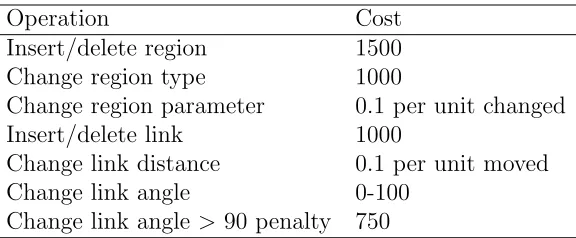
2.1 This table presents the graph edit costs used for graph edit distance calculations in this manuscript. . . 21
2.2 Evaluation of conversion equations to generate fitness values from graph edit distance values. The first row presents the data for the graph of the target individual. The first and second columns of the table show the ID and the image of the morphology graph. The third column presents the graph edit distance value obtained from comparison of the graph against the target graph using graph edit distance algorithm. The fourth through the ninth column show the fitness value produced by plugging in the constant in the column header into Equation 2.1. . . 27
7.1 Single cut morphology experiment results for simulation snapshot to graph conversion and graph edit distance comparison . . . 57
7.2 Threshold value influence on snapshot to graph conversion algorithm . . 59
7.3 Comparison of fitness function landscapes to the ideal fitness function landscape. . . 69
The first column shows the name of the landscape analyzed. DiffDist refers to the difference distributions evaluator and Graph to the graph edit distance evaluator. The second column presents the total number of flat surfaces in the landscape, the third column shows the percentage of the total landscape occupied by the biggest flat surface, and the last column shows the percentage of the landscape occupied by the flat surfaces. . . 70
7.5 Statistics obtained from analyzing the roughness of the fitness land-scapes. The first column shows the name of the fitness landscape, and the second column shows the number of local maxima in the landscape. 71
7.6 The runtime of difference distribution histogram creator implementa-tions in C and Python for morphology in column one are shown in columns two and three, respectively. The speedup provided by the C implementation of the histogram creator is shown in column four. The last row of the table shows the average runtimes. . . 74
7.7 Difference distributions for morphologies with different gene knockouts performed. The first row in the table presents the difference distribu-tion data for the target morphology. . . 76
1.1 This figure depicts a classic planaria regeneration experiment involv-ing a transverse cut of an intact worm, followed by the regeneration products for each fragment. The real experiment is shown in (a) along with the (b) simulation and (c) graph representations. In each case, the second panel represents the worms immediately following the cut, whereas the third panel depicts the regeneration outcome at a later time. 11
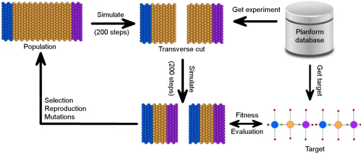
1.2 CSGA evolutionary search flow. . . 13
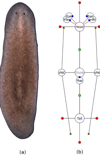
1.3 A wild-type planarian organism (a), along with its graph representation (b) in the Planform software tool. . . 15
1.4 A manipulation tree for an experiment involving removal of the head and tail regions. . . 17
centrations of cell-state indicators. The differentiate state of cells are color-coded to enable visual distinction of cells and the composition of a region: head (blue), trunk (yellow), and tail (purple). Within a given cell, the location of a given resource can be distributed between the internal compartment (e.g., cytosol) and the surface (e.g., membrane). Concentrations of representative resources inside (I) and on the surface (S) are provided. In this example, both Cell 1 and Cell 2 are assigned to a trunk state and Cell 3 is assigned to a trunk state, since the concentrations of the indicator molecules (iCell andtCell, respectively) for these states are the highest. . . 23
2.2 Pseudocode for connected component analysis recursive algorithm to separate a list of cells taken from the simulation snapshots into discrete morphology regions. . . 24
3.1 In this example of overlaying a cellular morphology with a graph mor-phology, the cellular morphology consists of three regions, head (red), trunk (blue), and tail (green), while the overlayed graph only has a head and a trunk. When the graph is overlayed with the cellular morphology, some of the cells do not match the type of the overlayed graph (colored in black). . . 30
3.2 Overlay difference fitness evaluator . . . 31
3.3 Sample conversion of a two-node morphology graph into lines. Three point types calculated during the conversion algorithm are indicated. . . 34
4.2 Fitness calculation using difference distributions . . . 39
5.1 UML diagram for the Planform database morphology. . . 42
5.2 UML diagram for the Planform database experiment. . . 43
5.3 UML diagram for the Planform database reader. . . 44
5.4 UML diagram for the Planform database writer. . . 46
5.5 Sample SQLite queries to call to PlanformDB. . . 46
5.6 Sample calls of Python database writer functions. . . 47
6.1 The graphical user interface for the CellSim simulation platform. . . 49
6.2 Example of applying a PlanformDB experiment manipulation (injec-tion of Lysis) to a cellular model in CellSim. . . 50
6.3 UML diagram for the PlanformDB experiment manipulation applica-tor. . . 51
6.4 Pseudocode for extraction of points falling inside the manipulation polygon formed by action points . . . 52
7.1 Fitness function evaluation on polar model with two gene regulatory regions removed independently and gradually returned. The x-axis shows the effect value of the knocked out regulatory region. The y-axis presents the fitness value assigned to the simulated model with a given promoter effect. The graph edit distance function fitness is shown in yellow, overlay in blue, and difference distributions in red. . . 63
head and tail regulatory region effects as well as its graph representation. 64
7.3 Fitness function evaluation of the polar model with hCell and tCell
promoters knocked out and gradually returned. . . 65
7.4 Fitness function evaluation of the polar model with lowhCellandtCell
decay rates in which hCell and tCell regulatory regions were knocked out and gradually returned. . . 67
7.5 A time series graph for an evolutionary search for a target capable of producing stable head and tail regions. . . 72
API– Application Programming Interface
CellSim– Cellular Simulation platform
CSGA – CellSim Genetic Algorithm
GA – Genetic Algorithm
GUI – Graphical User Interface
PlanformDB– Planform database
Subunit – A part of an abstracted cell in CellSim that facilitates cell growth and division
CHAPTER 1
INTRODUCTION
1.1
Problem Description
Robust regulatory control of organism morphology, including tissue and organ regen-eration, appears in many different animal and plant kingdoms and species, and has been extensively studied and analyzed by scientists [7, 21, 22]. Despite extensive effort and focus on this core problem in biology, and bringing to bear the incredibly powerful modern analytic tools developed by molecular biologists and bioninformaticians, the problem of deriving, understanding, and learning to control the robust, large-scale patterning properties of complex systems from the data about its components is yet to be solved.
features guiding the regulatory and patterning properties of planarians remain largely unknown. An especially interesting feature of planaria worms that has been puzzling the minds of scientists for over 200 hundred years is the flatworm’s ability to recover from even severe injuries. In 1776, Peter Simon Pallas discovered that bisecting a planarian organism did not kill it [35]. Instead, the two pieces of the cut worm regenerated into two intact worms (Fig. 1.1a). In 1898, Thomas Morgan showed that a cut worm piece constituting 1/279th of the total worm weight was able to regenerate into a new worm with many internal organs and a bilateral symmetry [31]. Since Pallas’ and Morgan’s discoveries, many more experiments have been performed on planaria aiming to understand the mechanics behind the animal’s remarkable regenerative capabilities [33], [23]. However, scientists still lack a complete understanding of the planarian regeneration process [23].
and fine tuning in order to explain these experiments. The problem of finding a regeneration model to fit all the experiments performed on planarians can be made more tractable by using computational tools to assist researchers in model formation, fine tuning, and testing.
A good example of such a tool is an evolutionary search algorithm combined with a cell-based modeling platform (CellSim Genetic Algorithm, or CSGA) used by the Andersen lab to discover and tune models of planarian regeneration [3]. Evolutionary search algorithms are inspired by biological evolution and based on the principle of survival of the fittest. Often regarded as generate-and-test algorithms, evolutionary algorithms use operators like mutation and crossover on populations of individuals to generate previously unseen individuals and test the goodness of these individuals via fitness evaluation [37]. An automated evolutionary algorithm can be used to combine and adjust the currently existing regeneration models to find a model that would be able to explain all the planarian regeneration experiments.
organized and mapped data, in which a directed acyclic graph (DAG) was used to represent is-a-part-of relationships between tissues and organs of a mouse embryo [5]. Maglia et al. described a generic anatomical ontology that can be applied to different amphibian species, where the anatomy of an organism is described as a semantic network consisting of concepts and relationships, such as is-fused-to, is-formed-from [27]. The utility of shape ontologies goes beyond the descriptions of species phenotypes: shape formalisms have been applied in clinical diagnostics and analysis of tumor growth [36].
One of the main reasons for the popularity of shape-based ontologies is flexi-bility. Shapes of organisms or organs described using a standardized language can be easily juxtaposed using computational methods. The computational flexibility of shape-based ontologies works in favor of automatizing the search for planarian regeneration models. Recently, the Levin lab at Tufts University developed a shape-based formalism for describing planarian morphologies as graphs of connected regions [26]. Flexible graph notation allows the organisms to be described in terms of nodes connected by links at specific angles. This formalism led to the implementation of a database for storing planarian morphologies and the experiments performed on planarians reported in the literature (PlanformDB) [25]. The database stores the ex-periment manipulations as a tree with planarian morphologies as leaves, which allows representation of a variety of experiments that can be performed on planaria. The Levin lab is working on populating this database (PlanformDB) with all experiments performed on planaria currently found in literature.
shape of the proposed regeneration model. While the majority of databases allow the experiments to be searched by keywords, the PlanformDB database enables searching experiments with the worm’s shape as the key. Graph comparison algorithms allow discovery not only of exact morphology matches but also ones that are similar to the sought-for shape. Graph-matching algorithms can be used to automate the validation of proposed regeneration models against the regeneration experiments found in literature. In addition to validation of regeneration models, the integration of PlanformDB can help create new models of regeneration if combined with an automatic tool to tweak the regeneration model parameters. CSGA perfectly fits the description of such a tool.
I have integrated the database of experiments and their outcomes (PlanformDB) into the CSGA evolutionary search engine with the aim of developing an automated system for searching and validating computational models of development. In this system, an experiment can be pulled from the database and simulated in the sim-ulation platform. In the past, in order to specify an experiment to be run in the cell-based platform, the user had to manually create a sheet of cells and specify operations to be performed on the morphology, such as cuts and injection of lysis or RNAi. This process of creating an experiment setup was painfully inefficient and slowed down the search for computational models of the planarian regeneration. The new automated system includes automatic access to the database for searching and pulling the experiments and morphological outcomes to use during the evolutionary search.
I developed a fitness function in which cellular outcome for a model generated by the simulation platform is converted into the graph representation and compared against the target individual from PlanformDB using the graph edit distance metric [12, 26]. The graph edit distance evaluator is a very flexible fitness function, since the graph formalism can be used in simulation platforms other than CellSim. However, a weakness of the graph edit distance evaluator is that it does not directly provide molecular targets for individual cells, but rather operates at the abstract level of a planarian morphology.
graph edit distance evaluator, and the overlay and difference distributions fitness functions. Each fitness function is evaluated by formally analyzing the roughness and flatness of the fitness landscapes produced by the evaluators. The utility of the fitness functions is also addressed by performing a simple evolutionary search for a target model capable of regenerating head and tail regions after a transverse cut is performed on the individual.
1.2
Thesis Statement
1.2.1 Objectives
The aim of this thesis is to automate the evolutionary search and discovery of com-putational models of planaria regeneration that faithfully reproduce experimental outcomes reported in the literature. Automation of the evolutionary search required development of flexible fitness metrics and integration with a database of existing experiments and experiment outcomes. This thesis fulfills the following objectives:
1. To develop robust techniques for comparing cellular models from the simulation platform to the search targets taken from the experiment database.
2. To automate the extraction of experiment manipulations and morphologies from the experiment database to the cellular platform.
1.2.2 Procedures
In order to achieve the proposed automation of evolutionary searches, the following components have been implemented and integrated with the CellSim simulation platform:
1. Fitness functions evaluate planarian regeneration models found during the evolutionary search.
(a) Graph Edit Distance Fitness Functionconverts a CellSim simulation snapshot into a graph representation. The converted graph is compared against the target morphology from PlanformDB using a graph edit dis-tance comparison technique [32] to yield the fitness value. The graph edit distance algorithm was originally integrated and implemented to interface with PlanformDB in C++ by Dr.Daniel Lobo as a part of Planform pro-gram [24]. This work integrates the C++ implementation of the algorithm with the Python implementation of the CellSim simulation platform and the CellSim Genetic Algorithm evolutionary search platform.
(c) Difference Distribution Fitness Function uses a statistical method developed by Robert Osada that creates distribution signatures for both the target morphology represented as a cellular snapshot and the CellSim simulation outcome [34]. The two signatures are compared to yield the fitness value that will guide the evolutionary search. This fitness function, originally implemented by Dr. Timothy Andersen and Dr. Jeffrey W. Habig in Python, is very slow and inefficient due to the limitations of the Python interpreted language. This work improves the fitness function by converting it into the C programming language, and thus greatly speeds up the comparison process.
The graph edit distance and the overlay fitness functions interface directly with the PlanformDB and pull the search targets from the database. The difference distribution fitness function uses a cellular snapshot as the target, so it does not interact with PlanformDB.
2. Experiment manipulation applicatorautomates performing of experiment manipulations from the experiment database, such as cuts, on the cellular model in the simulation platform.
3. Database readerextracts morphologies and experimental manipulations from the experiment database.
This work provides the capability of saving unique models found during the search to a morphology database associated with the current search.
1.3
Modeling a Classic Planaria Regeneration Experiment
To give a graphical motive for the automation of the evolutionary search, an exam-ple of non-automated set up for running regeneration experiments on a simulation platform is presented. As shown in the classic regeneration experiment (Fig. 1.1a), when a worm is bisected laterally, the resulting fragments lack a head or tail region. Each fragment has the potential to regenerate into independent, intact worms with the appropriate shape and architecture over the course of roughly ten days. As a validation of the cell-modeling platform (CellSim) for studying planaria regeneration, Dr. Jeff Habig of the Andersen lab developed a model by hand that simulated these simple experiments.
In the experiment, a simple worm architecture of 420 rectangularly arranged cells is used as an abstraction for an intact worm (Fig. 1.1b). At the beginning of a simulation, the head, trunk, and tail regions of the simulated worm are defined by manually injecting one of three indicator resources into the appropriate cells (head,
that should be injected by manual calculation of the rectangular region coordinates in the simulation where the cells are present. After the injection ofLysis, simulations consisting of two worm fragments are advanced 200 steps prior to evaluating the emergent outcomes.
As shown, the manual set up of even a simple experiment can be time-consuming. In order to simulate the many experiments described in the literature, some level of computational automation should be achieved.
1.4
Tools
1.4.1 Computational Platform and Evolutionary Search
Figure 1.2: CSGA evolutionary search flow.
CellSim to represent three main regions of a planaria worm, head, trunk, and tail, respectively. Figure 1.1b shows worms simulated using one subunit cells.
be of a particular representation. For example, the difference distribution fitness function uses a hand-crafted CellSim simulation snapshot as the target morphology.
1.4.2 A Database for Storing Planarian Experiments
The automation of search for the models of planarian regeneration that fit all the pla-narian experiments reported in the literature would be intractable without automatic access to the described experiments and outcomes. Lobo et al. developed a graph ontology for efficient storage, search, and mining of the regenerative experiments performed on planaria worms [24]. Planform formally encodes a wide range of morphologies, manipulations, and experiments. Instead of relying on imprecise and ambiguous natural language descriptions of worms, Planform formalizes planarian phenotypes using labeled mathematical graphs. A graph is an abstract representation of a set of objects that can be connected to each other via edges. In Planform formalism, the graph nodes represent body regions, while the edges describe the adjacency between two regions. Nodes and edges can store geometric characteristics of the worm anatomy, such as body region type, overall shape and size of regions, the rotation of organs, and other properties.
Figure 1.3: A wild-type planarian organism (a), along with its graph representation (b) in the Planform software tool.
+90, +180, and +270 degrees with respect to the direction of the edge (head and tail regions in Figure 1.3b); regions connected to more than one region have a parameter for each bisector of every two consecutive edges (trunk region in Figure 1.3b). The formalism can also represent organs, such as a ventral nerve cord, brain, and eyes, as shown in Figure 1.3b; however, the organs are beyond the scope of this work and will not be discussed here.
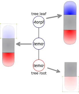
In addition to the formalism describing the shapes of planarians, the Levin lab introduced formalism for experiment manipulations. The formalism includes four basic manipulation types: remove (an area of the organism is cut out and discarded), crop (an area of the organism is cut out and the rest is discarded), and join (two worm pieces are grafted together). The manipulations performed in an experiment are abstracted as a mathematical labeled tree, in which the nodes represent basic manipulations and the edges connect manipulation outputs and inputs. The leaves of the manipulation tree represent the morphologies used to start the experiment, while the root of the tree presents the morphology whose regenerative capabilities are tested. Figure 1.4 shows a simple experiment tree consisting of three nodes - one is the starting morphology, and the rest are cuts performed on it. The root of the tree is a morphology whose head and tail regions have been removed.
Figure 1.4: A manipulation tree for an experiment involving removal of the head and tail regions.
1.4.3 A Sample Regeneration Model
One of the most interesting properties of planaria regeneration is their ability to robustly regenerate head and tail regions in the correct orientation relative to the starting worm. The Andersen lab set to explore the problem of how the worm is able to determine whether the head, or tail (or both) is missing, and the proper location for regeneration of the missing parts - without the added complexity of regenerating other structures, such as eyes, intestinal tract, and nerve cord. To explore this problem, and to facilitate the evaluation of different fitness metrics, a simplified model of planarian regeneration has been hand-designed by the Andersen lab that utilizes cell polarity as the basis for regeneration of the correct anterior and posterior ends. The polarity of each cell is established using hPole and tPole resources that the cell accumulates in opposite ends. The model is composed of a flat sheet of 168 cells arranged as a rectangular abstraction of an intact worm. Every cell in the polar model is autonomous but is controlled by an identical genetic network and each cell knows exactly where the head and tail (north and south) regions are located in relation to itself due to its internal polarity. Head, trunk, and tail regions in this model are represented by cell state indicator molecules,hCell,iCell, andtCell, whose homeostasis is ensured by a set or promoter genes.
CHAPTER 2
GRAPH EDIT DISTANCE FITNESS FUNCTION
2.1
The Graph Formalism for Comparing Worms
The graph edit distance is defined as the minimum number of distortions required to transform one graph into another graph. These distortions are referred to as graph edits, where each edit has a defined cost associated with it [32]. A particular sequence of edit operations required to transform one graph into another is called an edit path, and the total cost of the edit path is its graph edit distance. Graphs that are similar to each other typically have small edit distances, whereas dissimilar graphs have large edit distances. The cost of each type of graph edit operation varies and is dependent upon the perceived severity of the operation. For example, the deletion of a node from a graph is generally viewed as having a higher cost than a node parameter change. Thus, the graph edit distance can be used as a similarity measure to compare and order individuals within a population, and thus serve as a metric within a fitness evaluation to guide the evolutionary search process.
Dr. Daniel Lobo adapted the graph edit distance algorithm to be used with the planarian formalism graphs in PlanformDB [24]. The graph edit distance costs used in the algorithm implementation are described in Table 2.1. The penalties are most severe when differences exist between region numbers and connectivity than for region size and linkage parameters.
Operation Cost
Insert/delete region 1500 Change region type 1000
Change region parameter 0.1 per unit changed Insert/delete link 1000
Change link distance 0.1 per unit moved
Change link angle 0-100
Change link angle >90 penalty 750
As a part of this thesis, the C++ implementation of graph edit distance algorithm has been incorporated with the CellSim simulation platform. Since the simulation platform is implemented in Python, a Python to C++ interface has been developed to pass the Python graph objects as parameters to the C++ graph edit distance library. The interface between the simulation platform and graph edit distance library uses the ctypes foreign function library, which includes C compatible database types and capability of calling functions inside DLLs and shared libraries.
2.1.1 Design of a Connected Component Analysis Algorithm to Convert
Cell Simulation Output into Graph Representations
Figure 2.1: The assignment of a cell to a state depends on the molecular concen-trations of cell-state indicators. The differentiate state of cells are color-coded to enable visual distinction of cells and the composition of a region: head (blue), trunk (yellow), and tail (purple). Within a given cell, the location of a given resource can be distributed between the internal compartment (e.g., cytosol) and the surface (e.g., membrane). Concentrations of representative resources inside (I) and on the surface (S) are provided. In this example, both Cell 1 and Cell 2 are assigned to a trunk state and Cell 3 is assigned to a trunk state, since the concentrations of the indicator molecules (iCell and tCell, respectively) for these states are the highest.
state if its concentration of iCell is greater than hCell and tCell, as shown in Figure 2.1. The approach of assigning a cell to a region based on the highest concentration of an indicator resource is a simplification of reality, since many more factors may go into differentiation of a cell in an organism. Chapter 3 examines a more complex way of evaluating a cell’s region type.
ProcessConnectedComponents(snapshot):
list = new list of connected components for each unprocessed cell c in snapshot comp = new connected component add c to comp
set c as processed
GatherConnected(c, comp, snapshot) add comp to list
for comp in components:
calculate parameters for comp
GatherConnected(c1, comp, snapshot):
for each unprocessed cell c2 in snapshot if c1 and c2 are connected:
if c1 and c2 are not of the same type: mark c1 and c2 as border cells else:
add c2 to comp set c2 as processed
GatherConnected(c2, comp, snapshot)
Figure 2.2: Pseudocode for connected component analysis recursive algorithm to separate a list of cells taken from the simulation snapshots into discrete morphology regions.
The ProcessConnectedComponents function iterates through all cells and calls the GatherConnected function for each unassigned/marked cell.
connected, but are assigned to different regions because they are of different types, those cells are identified as border cells. Border cells are used to determine which regions are linked to each other.
Once each cell in the snapshot is assigned to a specific region, links between regions are calculated. The algorithm determines how many neighbors each region is connected to using the border cells found during the recursive process in Algorithm 2.2, and creates links between the connected regions. Two regions are be considered linked if they share border cells.
By the graph formalism, each link between regions is parametrized by the distance between the connected regions’ centers, the angle of the link measuring its tilt relative to the x-axis, and the location along the link where the two regions meet. The number of parameters for a region depends on the number of links it has. A component parameter is defined as the Euclidean distance from the center of a region to a region border in a specific direction. The center of a region is calculated by averaging the spatial centers of every cell in a particular region. The border of a region is calculated by finding the furthermost cell in a specific direction.
2.1.2 Graph Edit Distance as a Fitness Function
Since the GA is designed to evaluate fitness values in the range of 0.0 to 1.0, the graph edit value cannot be used by itself to measure the fitness of simulation outcomes, and thus is converted as shown in Equation 2.1.
f itness= 5000
(distance+ 5000) (2.1)
Initially, the simple inverse function of 1/(graph edit distance) was used to obtain the GA fitness values. However, the fitness function values in such cases tended to be very small even for relatively similar graphs due to sensitivity caused by the large edit penalties in Table 2.1.
To come up with an equation for converting graph edit distance values to fitness values that is capable of producing more intuitive fitness values, several morphology graphs were evaluated using the graph edit distance fitness function. The graph edit distance value for the tested graphs was converted into a value between 0.0 and 1.0 using Equation 2.1 with different constants in the range between 1 and 10000. Constants above 10000 were excluded from the evaluation on the basis of generating high fitness values for individuals with morphologies very dissimilar to the target.
Table 2.2: Evaluation of conversion equations to generate fitness values from graph edit distance values. The first row presents the data for the graph of the target individual. The first and second columns of the table show the ID and the image of the morphology graph. The third column presents the graph edit distance value obtained from comparison of the graph against the target graph using graph edit distance algorithm. The fourth through the ninth column show the fitness value produced by plugging in the constant in the column header into Equation 2.1.
ID Graph Distance 1 500 1000 3000 5000 10000
0 0.0 1.0000 1.0000 1.0000 1.0000 1.0000 1.0000
1 5009.0 0.0002 0.0908 0.1664 0.3746 0.4996 0.6663
2 7009.0 0.0001 0.0666 0.1249 0.2997 0.4164 0.5879
3 10008.8 0.0001 0.0476 0.0908 0.2306 0.3331 0.4998
4 5008.3 0.0002 0.0908 0.1664 0.3746 0.4996 0.6663
5 2000.0 0.0005 0.2000 0.3333 0.6000 0.7143 0.8333
6 2000.0 0.0005 0.2000 0.3333 0.6000 0.7143 0.8333
7 10000.9 0.0001 0.0476 0.0909 0.2308 0.3333 0.5000
8 10008.8 0.0001 0.0476 0.0908 0.2306 0.3331 0.4998
9 1698.4 0.0006 0.2274 0.3706 0.6385 0.7465 0.8548
10 1698.4 0.0006 0.2274 0.3706 0.6385 0.7465 0.8548
11 1000.0 0.0010 0.3333 0.5000 0.7500 0.8333 0.9091
12 2504.8 0.0004 0.1664 0.2853 0.5450 0.6662 0.7997
The constants of 500 and 1000 both produced very low values to the individuals tested, and thus were not optimal for the fitness conversion equation. The constant of 10000, on the contrary, yielded fitness values that were too high and did not maximize the differences between fitness values. In the last column of Table 2.2, which corresponds to the constant of 10000, the fitness values range from .49 to 1.0, which is not a very large fitness range for the individuals tested.
CHAPTER 3
OVERLAY FITNESS FUNCTION
3.1
Comparing Two Morphologies by Overlaying a Graph
with a Blob of Cells
The overlay fitness function calculates the best fit of a morphology graph to a cell-based model as shown in Figure 3.1. To create an overlay, the graph is scaled so that the graph fits inside of the cellular morphology and matches the width of the height of the morphology. For each cell in the cell-based morphology, the closest graph region of the overlayed graph is found. The cell gets assigned a subfitness based on how close the cell is to becoming the expected graph region.
Figure 3.1: In this example of overlaying a cellular morphology with a graph mor-phology, the cellular morphology consists of three regions, head (red), trunk (blue), and tail (green), while the overlayed graph only has a head and a trunk. When the graph is overlayed with the cellular morphology, some of the cells do not match the type of the overlayed graph (colored in black).
Classic experiments on planaria worms involve cuts separating a whole worm into several parts. For example, if a transverse cut is performed on a planarian, as shown in Figure 1.1, two cut pieces are expected to regenerate into complete worms. Therefore, to evaluate the effectiveness of the regeneration model, each of the regenerated pieces needs to be compared to the target.
OverlayDifferenceEvaluator(snapshot, graphList): Convert the cellular snapshot to blobs Sort blobs based on their centers Let cellSellsubfitnessSum = 0 For each blob:
Convert corresponding graph from graphList into 2D lines For each cell in the cellular morphology snapshot:
Find closest graph line to the cell
Set expectedRegion to the region of closes the graph line Calculate the cell subfitness
Add the cell subfitness value to cellSellsubfitnessSum return cellSellsubfitnessSum / number of cells in a snapshot
Figure 3.2: Overlay difference fitness evaluator
list of cells. Since an overlay needs to be calculated for each cut up piece, or blob, the cells in the snapshot cell list get separated into lists of blob cells. Each blob in the blob list is matched with a corresponding graph in the list of target morphology graphs provided by the user. Knowing the exact order of the blobs, the user can provide the correctly ordered graph list constituting the target morphology, so that the first blob is compared against the first graph, and so on. Providing a list of graphs instead of one graph with several subgraphs was required because the graph ontology of PlanformDB does not give any information about relative location of disconnected subgraphs.
molecule and the maximum concentration of an indicator molecule in a cell.
subf itness=max( conc(target−mol)
conc(mol−with−maximum−concentration),1) (3.1)
The final fitness of the model in the overlay evaluator is calculated by dividing the sum of subfitness values for every cell in the organism by the number of cells.
3.2
Graph-to-Line Conversion
To calculate an overlay of a graph to a cellular blob, the dimensions of the graph and the blob need to match. In the CellSim simulation platform and Planform graph formalism, the coordinate systems are arbitrary and carry no spatial meaning. For example, in the database and the simulation platform, the distance of 1 can mean the distance in millimeters, centimeters, etc. Due to the lack of spatial meaning of the coordinate systems, cellular and graph morphologies can be scaled in order to be matched and compared to each other without any loss of information.
The graph formalism used to encode morphologies in the experiment database stores morphology regions as graph nodes with parameters describing the general node shape. Graph node links contain information about how far away connected nodes are from each other and what their angle position is. For overlay to cover as much of the cellular worm as possible, the graph is expanded geometrically through conversion of the graph nodes into connected lines tracing the silhouette of the graph.
and links need to be projected into an x-y coordinate system. The algorithm randomly takes a node in the graph and assigns its center to the (0,0) coordinate. The coordi-nates for the parameter points defining the shape of the node are calculated based on the node’s center. Using the first node’s center coordinate and the distances to the nodes this node is connected to, the algorithm recursively assigns the coordinates to the rest of the nodes in the graph. Once the graph nodes, parameters, and links have been projected into the x-y coordinate system, the points defining the silhouette of the graph are computed.
The points in the graph-to-line conversion algorithm can be of three types: pa-rameter points, link points, and points between border papa-rameters. Figure 3.3 shows a sample graph with the three point types indicated. In the graph formalism, a parameter for a region indicates the distance from the region center to the parameter point in a specific direction. Parameter points lie at the end of the parameters. Link points lie on a border line that connects the centers of two nodes. For each parameter point on a border between two regions, an additional point is calculated to help define a more accurate shape of the worm for the overlay. In the figure, it is called a point between border parameters. The calculated points for a node get connected into lines and can be used to create the overlay.
Figure 3.3: Sample conversion of a two-node morphology graph into lines. Three point types calculated during the conversion algorithm are indicated.
CHAPTER 4
DIFFERENCE DISTRIBUTIONS FITNESS FUNCTION
4.1
Comparing Two Morphologies by Calculating Difference
Distributions of Their Resources
While abstracting the worm morphology into regions allows a very flexible means of comparison between the simulation platform outputs and the target PlanformDB morphology, the graph representation may be too coarse-grained in certain instances as discussed in Chapter 2. As an alternative to abstracting the cellular representation of the worm in the simulation platform, the simulation outcome can be viewed as a multidimensional vector, consisting of multiple features, such as molecular concentra-tions and individual cell locaconcentra-tions. Vectors for the simulation output and the target may vary significantly, and so flexible comparison algorithms are needed to calculate the differences between multidimensional vectors describing two distinct worms.
containing holes in the surface. To mitigate the limitations of traditional shape comparison algorithms, Osada et al. proposed an algorithm to compare arbitrary 3D models using shape distributions [34]. Osada et al.’s algorithm calculates a signature for each 3D shape by sampling from a shape function, which measures geometric properties of a 3D model. For example, the samples for a shape can be gathered by calculating distances between 3D points in the shape and then normalized into a distribution. The normalization of a shape distribution allows Osada et al.’s algorithm to be translation, rotation, and size-invariant. To compare two 3D shapes, Osada et al.’s algorithm calculates the difference between the normalized distribution signatures for the shapes.
Just like 3D shapes, simulation outcomes of planaria regeneration models are multidimensional objects that may have missing structures, such as cells, genome regulatory regions, or metabolic equations. Simulation outcomes may also be rotated differently than the target due to the experiment setup, and thus significantly vary from the target in a structural, though not necessarily in an functional, way. In this work, Osada et al.’s difference distribution algorithm has been incorporated as a GA fitness function that can compare simulation outcomes to the target outcome. The difference distribution fitness evaluator computes a statistical signature, or a difference distribution histogram, for the internal state of the worm by considering concentrations of specific molecules and locations of individual cells. Fitness value of the simulation outcome is calculated by comparing the difference distribution histograms of the simulation outcome and the target outcome.
creates the normalized difference distribution histogram for the simulation outcome (createDistribution).
In the default implementation, distances between two points are taken exhaus-tively for every pair of cells. The samples gathered include distances between the cell centers of mass and molecular concentrations of cells. For each sample, the distance between two cells is computed by calculating the sum of squared differences of cells’ locations and molecular contents (processCells).
As an alternative to exhaustive sampling, stochastic sampling can be specified in which only a certain number of measurements are taken for randomly chosen cells. To get a more precise distribution of the simulation outcome, a subunit-to-subunit distance can be computed. The subunit-to-subunit-to-subunit-to-subunit difference processor uses the processCellSubunits function, which iterates over all subunits in two cells and compares the subunits’ locations and molecular contents. The subunit-to-subunit processor is more compute intensive, but it also allows a more accurate representation of the simulation model’s shape and location of molecular contents.
The obtained samples are used to construct a difference distribution histogram by counting how many samples fall into each of B fixed size bins (calculateDistribution in Algorithm 4.1). The number of samples that falls in each bin is normalized by dividing the sample count for a bin by the total number of samples taken.
distribution():
takeSamples()
createDistribution()
takeSamples():
for cell1 in cells:
for cell2 in cells:
processCells(cell1, cell2)
processCells(cell1, cell2): sum = 0;
sum += calcSquaredDifference(cell1.x, cell2.x) sum += calcSquaredDifference(cell1.y, cell2.y) sum += calcSquaredDifference(cell1.z, cell2.z) for each molecule mol:
sum += calcSquaredDifference(
mol concentration in cell1, mol concentration in cell2) add sum to the list of measurements
calculateDistribution():
let binCounts be an array of size B
let measurementCount be the size of measurements for each measurement in measurements:
binCountIndex = calculate the bin for the measurement binCounts[binCountIndex]++
normalize each binCount in binCounts by measurementCount
absoluteDifference(a,b): return |a-b|
calculateFitness()
//get a list of absolute differences of two bins
absoluteDifferences = map(absoluteDifference, bins1, bins2)
differenceSum = sum all the absolute differences in the absoluteDifferences return 1 - differenceSum/2.0
Figure 4.2: Fitness calculation using difference distributions
As an alternative to Minkowski LN norm, distribution histograms can be compared
CHAPTER 5
EXPERIMENT DATABASE READER AND WRITER
The PlanformDB of planarian experiments is an invaluable tool for searching the ex-periments reported in the literature. To provide access to PlanformDB and the ability to add new experiments into the database, the Levin lab implemented an executable GUI program called Planform that allows users to view, search, and manually edit database morphologies and experimental manipulations [24]. Being the sole access point to the database, Planform allows for only manual modification of the database and does not provide APIs to read and write to the database programmatically.
Without programmatic access to PlanformDB, utilizing the database in the evo-lutionary search and the simulation platform is inefficient. Running experiments, injecting worms with Lysis, and creating cellular morphologies by injecting head and tail indicators would be performed manually and thus would be time-consuming. To alleviate this problem and allow automatic retrieval of information pertinent to planarian experiments, a database reader and writer that can programmatically access and manipulate PlanformDB have been created.
morphology and an experiment, respectively. The structure of these classes reflects the database schema of PlanformDB described in Section 1.4.2.
5.1
Experiment Database Reader of Morphologies and
Ex-periments
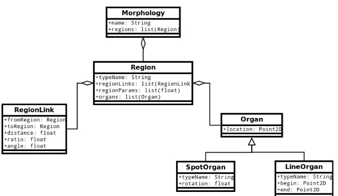
Just like in PlanformDB, the main Python class representing a planarian is called Morphology, as shown in Figure 5.1. Each morphology consists of interconnected regions (class Region) such as head, trunk, and tail. A region knows exactly what other regions it is connected to by maintaining a list of region links (class RegionLink). A region also knows what organs are contained within it, such as spot organs (eyes, brain lobe, pharynx) and line organs (ventral nerve cord). The current work did not deal with morphologies containing organs; however, the implementation of the classes was designed so that in future studies organs can be incorporated into the the evolutionary search.
Figure 5.1: UML diagram for the Planform database morphology.
morphology action (class MorphologyAction). The four action classes in Python were implemented to inherit from the base ManipulationAction class, since they all share attributes, including the name of the manipulation and the reference to the child manipulation action. CropAction and RemoveAction objects store a list of points representing an area that should be respectively cropped or removed from a planarian morphology. The JoinAction represents the grafting of two manipulation action subtrees, while the MorphologyAction simply stores the reference to the Morphology object on which the manipulations are to be performed.
Figure 5.2: UML diagram for the Planform database experiment.
connect to an SQLite database and call SELECT statements on it to retrieve values from a specified table. DBExperimentReader and DBMorphologyReader classes use the DBReader class to access the PlanformDB and extract values pertinent to the experimental manipulations performed on planaria as well as planarian morphology graphs.
Figure 5.3: UML diagram for the Planform database reader.
the Python objects representing an experiment (processExperiment), a manipulation (processManipulation), a tree of manipulation actions (processActionSubtree), as well as the specific manipulation actions (processMorphologyAction, processRemoveAc-tion, processCropAcprocessRemoveAc-tion, processJoinAction). The created Experiment object can then be used by the manipulation applicator described in Chapter 6 to perform the PlanformDB experiment on the cellular morphology from the simulation platform.
5.2
Experiment Database Writer of Morphologies
During the evolutionary search, large numbers of unique individuals are generated. Even though the individuals produced by the genetic algorithm are automatically evaluated by the fitness function and selected for further generation cycles, extra human checking may be needed to examine the progress of the evolutionary search. Since graphical representation of planarian morphologies is a lot more user-friendly than the XML files describing regeneration models in CSGA and CellSim, it is deemed useful to save unique individuals discovered by the GA into the PlanformDB. To this end, a Python module has been designed to write morphology Python objects to a user-specified database. Embedded in the evolutionary search, this module automatically saves unique morphologies to a database tied to the currently performed search.
Figure 5.4: UML diagram for the Planform database writer.
(1) SELECT Id FROM Morphology WHERE Name=’Wild type’ (2) INSERT INTO Morphology (Id, Name ) VALUES
(
(SELECT max(Id) FROM Morphology )+1, ’Wild type’
)
(3) DELETE FROM Morphology WHERE Id=’17’
Figure 5.5: Sample SQLite queries to call to PlanformDB.
delete morphology graphs with specified names to and from the database. These two functions are implemented using three basis functions, insert, select, and delete, which in turn execute the SQLite’s basic INSERT, SELECT, and DELETE commands.
(1) select(
location = "Morphology", paramToSelect = "Id",
restriction = "WHERE Name=’" + "Wild type" + "’" )
(2) insert(
location = "Morphology", paramList = "Name",
valueList = [’Wild type’], restriction = ""
) (3) delete(
location = "Morphology",
restriction = "WHERE Id=’" + str(17) + "’" )
CHAPTER 6
AUTOMATED EXPERIMENT EXTRACTION AND
APPLICATION
The CellSim simulation engine provides a simple, easy-to-use graphical tool to select and manipulate cells as shown in Figure 6.1. With this tool, a user can inject various resources, such as Lysis and region indicators, into selected cells.
Figure 6.1: The graphical user interface for the CellSim simulation platform.
Figure 6.2: Example of applying a PlanformDB experiment manipulation (injection of Lysis) to a cellular model in CellSim.
The manipulation application module consists of three classes, each class respon-sible for a single task. The first class translates manipulation action points from the PlanformDB coordinate system to the CellSim coordinate system. The second class calculates what cells in the manipulated morphology fall within the area inside the polygon formed by the action points. The third class acts as the coordinator and keeps track of the PlanformDB experiment manipulation and the cellular morphology.
Figure 6.3: UML diagram for the PlanformDB experiment manipulation applicator.
manipulationApplicator = ManipulationApplicator(experiment, cells) cells = manipulationApplicator.getCellsToManipulate()
class ManipulationApplicator: getCellsToManipulate():
get experiment action points for each point in points:
PointToPointTranslator.translate(point)
return CellsGeometryCalculator.getCellsInsidePolygon(translated points)
class PointToPointTranslator: tralslate(point):
rescalePoint(point) movePoint(point)
rescalePoint(point):
point.x = point.x * width ratio point.y = point.y * height ratio
movePoint(point):
point = point + worms’ center location in CellSim
class CellsGeometryCalculator:
getCellsInsidePolygon(polygon):
initialize an empty list as cellsInsidePolygon for each cell in morphology cells:
if not cellIsOutsidePolygon(cell, polygon): add cell to cellsInsidePolygon list return cellsInsidePolygon list
cellIsOutsidePolygon(cell, polygon):
create a ray going from (cell x, cell y) to (infinity,cell y) for each polygon side of polygon:
if polygon side intersects ray: return false
return true
Figure 6.4 shows the pseudocode to extract cells falling inside the polygon for a region removal experiment. The pseudocode to extract cells outside the polygon for a crop experiment is very similar and will not be discussed here. The algorithm starts by creating a ManipulationApplicator object, and calling the getCellsToMa-nipulate function. The getCellsToMagetCellsToMa-nipulate function retrieves action points from the Experiment object and translates them into an x, y, z coordinate system by calling PointToPointTranslator’s translate function. Translation of a point involves re-scaling of the point’s x and y coordinates by width and height ratios and moving the point by the cellular worm’s center. The height and width ratios used in point scaling are computed by dividing the cellular worm’s height by graph worm’s height and cellular worm’s width by graph worm’s width, respectively. An action point is moved to correspond to the CellSim worm’s center since in PlanformDB morphologies are always centered at the (0,0) coordinate, while in CellSim the center of the worm may be any coordinate.
CHAPTER 7
RESULTS
7.1
Evaluation of the Cellular Snapshot-to-Graph
Conver-sion Algorithm
During an evolutionary search, large numbers of unique individuals are generated and must be evaluated against the target individual encoded in the database. To ensure that converted graph representations are intuitive and to evaluate the use of the graph edit distance metric for ordering individuals in the population, an evaluation of the conversion algorithm was performed. To this end, a number of worms with distinct morphologies was generated by hand using the simulation platform, and their snapshots were converted into graph representations using the conversion algorithm. The simplest individuals that can be represented by the simulation platform include worms with discrete regions, whereas more complicated morphologies consisting of regions contained within other regions can also exist. Just considering the basic morphologies, the number of individuals that can be formed and the fitness landscapes for the genetic algorithm are infinite, and therefore the conversion algorithm was tested using simple individuals before considering more complicated morphologies.
included two fragments to simulate the state of worms following a single transverse cut. Each worm was generated by injection of the appropriate cell-state resource (i.e. hCell, tCell, and iCell) to create the desired regions within the worm frag-ments, resulting in different permutations of head, tail, and trunk regions. Every test morphology was converted to a graph (Table 7.1, Morphology Graph) using the connected component analysis conversion algorithm. No discordance was found between the graphs generated by the conversion algorithm and those expected upon visual inspection of the simulation output. Thus, the algorithm was working as expected on these simple morphologies.
During an evolutionary search, the genetic algorithm needs to compare individuals to the target and reward those individuals that are most likely to turn into the target, that is, possess a reaction network capable of proper regeneration. The genetic algorithm assigns fitness values based upon how evolutionally close the individual is to the target, with closer individuals getting higher fitness values. A fitness value of 1.0 is awarded to an individual with a perfect match to the target and is the ultimate goal of a search. Thus, the graph edit distance was calculated between each test individual and the target and those values were converted into a fitness value (Table 7.1).
Table 7.1: Single cut morphology experiment results for simulation snapshot to graph conversion and graph edit distance comparison
ID Simulation Snapshot Morphology Graph Fitness Value Edit Distance
0 1.000 0
1 0.500 5009
2 0.416 7009
3 0.333 10009
4 0.500 5008
5 0.714 2000
6 0.714 2000
7 0.333 10001
8 0.333 10009
9 0.746 1698
10 0.746 1698
11 0.833 1000
12 0.666 2505
genetic algorithm search indicates the target morphology has been found. Morphology 13 in Table 7.1 is a slight variation of the target morphology, where its heads are several cell layers thinner than the heads of the target, and as expected has the next best fitness value (0.998). In general, high fitness values for morphologies such as number 13 are expected as their regions are connected and oriented the same as the target. When compared to the target, morphologies that consist of three regions in each worm fragment received higher fitness values than morphologies having one or two regions. For example, morphology 6 was rated higher than morphology 4. Again, this is because the graph edit distance costs included a much larger penalty for the deletion of a region than with a change to the type of region.
Conversion of a simulation snapshot into the graph is an O(N2) algorithm where
N is the number of cells in an individual. The wild-type morphology had 420 cells, but since the transverse cut removed four rows of cells, the morphologies used in this experiment consisted of 364 cells. The conversion algorithm ran in less than 1.3 seconds for every morphology in Table 7.2. The run time of the graph edit distance calculation grows exponentially with the size of the graphs (number of nodes, or in our case to the number of regions in the two morphologies)[32]. However, since the number of regions in each morphology tested was at most 6, the graph edit distance algorithm finished in less than 1 millisecond for all morphologies.
7.1.1 Cell Connectivity Distance Threshold Effects on Region
Determi-nation
Threshold Snapshot Graph Fitness Edit Distance
1 1.000 0
1 0.250 15029
2 0.999 7
2 0.664 2528
3 0.999 6
Table 7.2: Threshold value influence on snapshot to graph conversion algorithm
simulation have radii of 0.5 units, the Euclidian distance between two adjacent cells can be as low as one. However, using a very rigid measure for identifying neighboring cells and determining the borders of regions can have dramatic effects on the graph conversion. For example, consider the morphology of the second individual shown in Table 7.2. In this individual, thin lines of trunk cells dissect the head and tail regions into a number of potentially distinct heads and tails if the borders are considered rigidly. Comparison of this individual with the target results in a very high graph edit distance due to the cost associated with having multiple heads. However, in the context of a evolutionary search, this individual may be very close to producing the target morphology.
1.0.
A second example highlighting the importance of this parameter to component gathering is presented at the bottom of Table 7.2. This worm represents a classic experiment that involves separating the head region into two fully-developed heads. These two heads are separated physically and should be classified as two-headed. A threshold parameter of less than three results in the desired graph conversion in our algorithm, whereas the larger value results in a worm with a single head.
These two examples show the necessity of a flexible parameter for determining local regions during a GA run. In the first case, a low threshold was shown to penalize a morphology that was very similar to the target, whereas a high threshold inappropriately favored a morphology containing a physical gap between head regions. An optimal threshold depends upon the modeling platform and project, but in this work and from an evolutionary perspective a threshold of two was optimal.
7.2
Evaluation of the Proposed Fitness Functions
evaluated. In the analysis performed, the evaluated entity is the polar regeneration model, and the variables are the regulatory region effects attached to head and tail promoter genes. Regulatory region effects control how much of a given molecule is being produced in maintaining homeostasis of the regeneration model.
Analysis of a fitness landscape involves examining how gradual the landscape is, considering that the most gradual fitness landscapes are the easiest to search. Gradual nature of a landscape can be assessed by examining the flatness and the roughness of the landscape. A flat landscape is considered to be undesirable because it does not provide a direction for the search to proceed, while a rough landscape with lots of local maxima is undesirable because the search may get stuck at the local maxima. In a rough landscape, the search will see the current solution as the best one compared to solutions surrounding it. Therefore, the most searchable fitness landscape is the one in which, at every landscape point, the slope provides search direction for better solutions.
The first step of evaluation was to analyze how knockouts of varying severity affect the fitness landscape formed by different fitness functions. A gene can be knocked out by setting the gene regulatory region effects to zero. Head and tail genes were knocked out from the polar regeneration model and then gradually returned back to the model by restoring a fraction of the regulatory region effects. The model was then simulated in the CellSim simulation platform and the outcome was evaluated against the target morphology using three fitness functions.
restored to the model until the gene regulatory region effects were the same as those of the original model. As a fraction of the regulatory region effect was restored to the model, the model was simulated in CellSim and evaluated using the three fitness functions.
In Figures 7.1(a) and 7.1(b), the difference distributions and overlay fitness values gradually rise with the increasing regulatory region effect and reach 1.0 when the regulatory region effect is the same as that of the target morphology. The graph edit distance evaluator has not performed as well as the overlay and difference distributions evaluators. The fitness line is not gradual, with many large dips present throughout. With the smaller regulatory region effects, the simulation often yields outcomes consisting of disconnected cells constituting a region. Due to the component gathering algorithm used in the graph edit distance evaluator to convert simulation outcomes to graphs, the disconnected region cells are converted into separate regions. The graph edit distance algorithm assigns large penalties to graphs with extra regions, thus lowering the fitness values of the simulation outcomes significantly, which explains the big fitness value drops in the figures.
(a) Fitness function performance on model with gradual restoration of an hCell regulatory region.
(b) Fitness function performance on model with gradual restora-tion of an tCell regulatory region.