METHOD FOR TRANSPORT ON THE SPHERE
by
Kevin Aiton
A thesis
submitted in partial fulfillment
of the requirements for the degree of
Master of Science in Mathematics
Boise State University
DEFENSE COMMITTEE AND FINAL READING APPROVALS
of the thesis submitted by
Kevin Aiton
Thesis Title: A Radial Basis Function Partition of Unity Method for Transport on the Sphere
Date of Final Oral Examination: 06 December 2013
The following individuals read and discussed the thesis submitted by student Kevin Aiton, and they evaluated his presentation and response to questions during the final oral examination. They found that the student passed the final oral examination.
Grady Wright, Ph.D. Chair, Supervisory Committee Donna Calhoun, Ph.D. Member, Supervisory Committee Inanc Senocak, Ph.D. Member, Supervisory Committee
This work was supported, in part, by the National Science Foundation (NSF)
under grant DMS-0934581 and also by the Boise State Mathematics Department
under the 2013 summer graduate fellowship.
I would like to express gratitude to Professor Grady Wright. He has been both
kind and patient. I would also like to thank the MOOSE development team at Idaho
National Laboratory for letting me work remotely so I could work on my thesis.
Finally, I would like to give gratitude to my family. Without their support, I would
not have been able to finish this thesis.
The transport phenomena dominates geophysical fluid motions on all scales
making the numerical solution of the transport problem fundamentally important for
the overall accuracy of any fluid solver. In this thesis, we describe a new high-order,
computationally efficient method for numerically solving the transport equation on
the sphere. This method combines radial basis functions (RBFs) and a partition of
unity method (PUM). The method is mesh-free, allowing near optimal discretization
of the surface of the sphere, and is free of any coordinate singularities. The basic idea
of the method is to start with a set of nodes that are quasi-uniformly distributed on
the sphere. Next, the surface of the sphere is partitioned into overlapping spherical
caps so that each cap contains roughly the same number of nodes. All spatial
derivatives of the PDE are approximated locally within the caps using RBFs. The
approximations from each cap are then aggregated into one global approximation
of the spatial derivatives using an appropriate weight function in the PUM. Finally,
we use a method-of-lines approach to advance the system in time. We analyze the
computational complexity of this method as compared to global methods based on
RBFs and present results for several well-known test cases that probe the suitability
of numerical methods for modeling transport in spherical geometries. We conclude
with possible future directions of the work.
ABSTRACT . . . v
LIST OF TABLES . . . viii
LIST OF FIGURES . . . x
LIST OF ABBREVIATIONS . . . xiii
LIST OF SYMBOLS . . . xiv
1 Introduction . . . 1
1.1 Radial Basis Function Interpolation . . . 2
1.2 The Shape Parameter . . . 4
1.3 Using RBFs to Solve Partial Differential Equations on the Sphere . . . . 7
1.4 Overview of Thesis . . . 11
2 RBF Partition of Unity Method (RBF-PUM) . . . 13
2.1 Constructing the RBF Partition of Unity Interpolant . . . 13
2.2 Choosing the Nodes and Patches . . . 16
2.3 Approximating the Surface Gradient Operators . . . 18
2.4 Computational Complexity of Constructing RBF-PUM Differentiation Matrices . . . 19
2.5 Sparsity of the RBF-PUM Differentation Matrices . . . 22
3 Numerical results . . . 30
3.1 Cosine Bell Test . . . 31
3.2 Deformational Flow Tests . . . 36
3.3 Stationary Vortex Roll-Up . . . 44
3.4 Computational Performance . . . 47
4 Future Work . . . 49
REFERENCES . . . 52
A Choosing Node Sets . . . 55
A.1 MD Points . . . 55
A.2 ME Points . . . 55
B Tables for n and q values . . . 57
B.1 Number of Nodes per Patch . . . 57
B.2 Number of Patches a Node Belongs to . . . 59
1.1 Examples of commonly used radial kernels. Here ε > 0 is called the
shape parameter. . . 3
2.1 Ratio of number of non zeros in a differentiation matrix compared to
our estimate and percent full the differentiation matrices are with q=3. 23
2.2 Ratio of number of non zeros in a differentiation matrix compared to
our estimate and percent full the differentiation matrices are with q=3.5. 24
2.3 Ratio of number of non zeros in a differentiation matrix compared to
our estimate and percent full the differentiation matrices are with q=4. 24
B.1 Mean and standard deviation of the number of nodes per patch with
q=3 . . . 58
B.2 Mean and standard deviation of the number of nodes per patch with
q=3.5 . . . 58
B.3 Mean and standard deviation of the number of nodes per patch with
q=4 . . . 59
B.4 Mean and standard deviation of the number of patches a node belongs
to with q=3 . . . 60
B.5 Mean and standard deviation of the number of patches a node belongs
to with q=3.5 . . . 60
to with q=3.5 . . . 61
1.1 Plots of the radial kernels found in Table 1.1. For each plot, the kernel
is ploted for shape parameter valuesε = 0.5,1,2. . . 5
2.1 Illustration of the nodes and patches used in the RBF-PUM for
in-creasing q with parameters N = 4096 and n = 100. Here the black
solid circles reperesent the nodes, blue spherical caps represent the
patches, and the red solid circles represent the centers of the patches.
The sparsity of the corresponding differentiation matrices is also shown
for each q. . . 25
2.2 Eigenvalues of the RBF-PUM differentiation matrix for the advection
operator corresponding to solid body rotation for the case ofN = 4096
nodes, a target condition number of tcone = 1012, and q = 4. The left
column shows the (scaled) eigenvalues of −D, corresponding to no
hyperviscosity (see Eq. 2.17). The right column shows the (scaled)
eigenvalues of −(D−µH), corresponding to the stabilized
differenti-ation matrix with hyperviscosity (see Eq. 2.18). For both value of n,
µ = 10−8. The black curve in all plots corresponds to the stability
domain of RK4 and the eigenvalues have been scaled by ∆t = 2π/1600. 28
3.1 Plots of the the solution and error using the GA kernel forN = 12544,
n= 144, ∆t= 2π/1600,µ= 8×10⁻⁹. . . 33
as a function of N and n, ∆t = 2π/1600, and tcond = 10 ; for the
GA kernel testµ= 5×10⁻¹¹ while for the IMQ kernel µ= 6×10⁻¹¹. . 34
3.3 Convergence plots of the cosine bell test using the GA and IMQ kernels
as a function ofN andn, ∆t = 2π/1600, andtcond = 1012;µ= 5×10⁻⁹
for both kernels. . . 35
3.4 Plots of the solution and error using non-smooth cosine bells with
the GA kernel for N = 20736, n = 100, ∆t = 5/2400, µ = 10−10,
tcond = 1014. . . 38
3.5 Convergence plots of the deformational flow test with cosine bell initial
condition using the GA and IMQ kernels as a function ofN andnusing
non-smooth cosine bells for ∆t= 5/2400, andtcond = 1014;µ= 10−10
for both kernels. . . 39
3.6 Convergence plots of the deformational flow test with cosine bell initial
condition using the GA and IMQ kernels as a function ofN andnusing
non-smooth cosine bells for ∆t = 5/2400 and tcond = 1012;µ = 10−8
for both kernels. . . 40
3.7 Plots of the solution and error using smooth Gaussian bells with the
GA kernel for N = 20736, n = 100, ∆t = 5/2400, µ = 2.5×10⁻¹⁰,
tcond = 1014. . . 41
3.8 Convergence plots of the deformational flow test with Gaussian bell
initial condition using the GA and IMQ kernels as a function ofN and
n using smooth Gaussian bells for ∆t= 5/2400 and tcond = 1014;µ=
2.5×10⁻¹⁰ for both kernels. . . 42
initial condition using the GA and IMQ kernels as a function of N
andn using smooth Gaussian bells for ∆t= 5/2400 and tcond = 1012;
µ= 10−8 for both kernels. . . 43
3.10 Plots of the solution and error of the stationary vortex roll-up test
with the GA kernel for N = 16384, n = 100, ∆t = 1/25, µ = 9.8×
10−12,t
cond = 1014. . . 45
3.11 Convergence plots of stationary vortex roll-up test using the GA and
IMQ kernels as a function of N and n for ∆t = 1/25 and tcond =
1014;for the GA kernel test µ= 9.8×10⁻¹², while for the IMQ kernel
µ= 10−11. . . 46
3.12 Convergence plots of stationary vortex roll-up test using the GA and
IMQ kernels as a function of N and n for ∆t = 1/25 and tcond =
1012;for the GA kernel test µ = 5×10⁻¹⁰, while for the IMQ kernel
µ= 6×10⁻¹⁰. . . 46
3.13 Plots for the cosine bell test for wall-clock time (sec) vs. N and
wall-clock time vs. relativel2 error using the GA kernel with ∆t= 2π/1600,
and tcond = 1014 and µ= 5×10⁻¹¹. . . 48
3.14 Plots for the deformational flow test with Gaussian bell initial condition
for wall-clock time (sec) vs. N and wall-clock time vs. relative l2
error using the GA kernel with∆t = 5/2400 and tcond = 1014 and
µ= 2.5×10⁻¹⁰. . . 48
GA – Gaussian
IMQ – Inverse multiquadric
PDE – Partial Differential Equation
RBF – Radial Basis Function
RBF-PUM – RBF-Partition of Unity Method
RK4 – Standard fourth-order Runge Kutta method
g
X For a real valued functiong :D→Rand a finite setX ={x1,x2, . . . ,xn} ∈D,
g
X = [g(x1), g(x2), . . . , g(xn)] T.
µ Hyperviscosity parameter
∆t Time-step
∇ Gradient operator in Cartesian coordinates
S2 The unit sphere in three dimensions.
CHAPTER 1
INTRODUCTION
Mathematical modeling of climate and weather often requires the numerical solution
of partial differential equations (PDEs) on the surface of the sphere. Several challenges
arise in solving these problems. First while these PDEs can often naturally be
parameterized in spherical coordinates, this can’t be done if the problem is intended
to be solved over the entire sphere without severe unphysical distortions near the
poles. This is because any two dimensional coordinate system on the sphere will have
at least one singularitiy. Second, these coordinate singularities manifest themselves as
apparent singularities in the differential operators of the PDE, complicating numerical
discretizations near the singularities. Third, the geometry of the sphere makes it
difficult to produce a regular grid or mesh that covers the sphere, as is required for
most numerical methods for PDEs. Even popular mappings like the cubed sphere
(mapping the faces of an inscribed cube to the sphere) introduce irregularities or
distortions in the grid that can effect numerical solutions.
Numerical methods based on Radial Basis Functions (RBFs) provide a promising
path to avoiding these issues [11, 12]. These methods can easily be expressed in
Cartesian coordinates allowing the PDEs to be solved directly on the sphere without
any coordinate singularities or singularities in the differential operator. They also do
they provide high-orders of accuracy (exponential or spectral) for smooth solutions.
The downside of these methods is that the computational complexity can be high
scaling like O(N2) for the global RBF method, whereN is the number of degrees of
freedom.
In this thesis, we develop a novel RBF method that reduces the computational
complexity to O(N), while still resulting in high orders of accuracy. We apply this
method to the numerical solution of the transport equation on the sphere. Transport
processes dominate geophysical fluid motions on all scales, so this is the first PDE
that new numerical methods for modeling climate and weather are tested on.
Below we briefly introduce RBF interpolation, as it is a major ingredient to our
new method. We then discuss the global RBF approach to solving the transport
equation from (1.6) since our new method follows a similar approach.
1.1
Radial Basis Function Interpolation
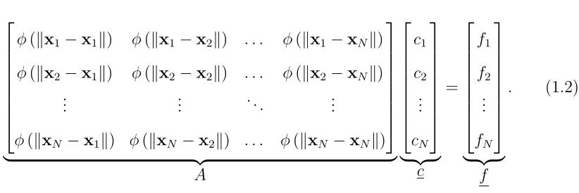
RBFs can be used for interpolating data{fi}Ni=1 ⊂Rsampled on a finite set of nodes X ={xi}Ni=1 ⊂Rd.The RBF interpolant s(x) :Rd→R is of the form
s(x) = N
X
i=1
ciφ(kx−xik), (1.1)
where φ : R → R is some radial kernel and k · k represents the Euclidian or
φ(kx1−x1k) φ(kx1 −x2k) . . . φ(kx1−xNk)
φ(kx2−x1k) φ(kx2 −x2k) . . . φ(kx2−xNk) ..
. ... . .. ...
φ(kxN −x1k) φ(kxN −x2k) . . . φ(kxN −xNk)
| {z }
A c1 c2 .. . cN
| {z }
c = f1 f2 .. . fN
| {z }
f
. (1.2)
We callAthe interpolation matrix. For certain types of radial kernels (such as the first
three entries of Table 1.1), Ais positive definite provided that the nodes are distinct
[3]. Thus, existence of a unique interpolant is guaranteed and the method is
well-posed. Considering that the interpolant is only dependent on the Euclidian distance
between the nodes the interpolant can easily be used for interpolating scattered data
in arbitrary dimensions, and on submanifolds ofRd such as the unit sphere S2 [19].
Table 1.1: Examples of commonly used radial kernels. Here ε >0 is called the shape parameter.
Name φ(r)
Gaussian (GA) e−(εr)2
Laguerre-Gaussian (LGA) 52 −(εr)2e−(εr)2
Inverse Multiquadratics (IMQ) 1 + (εr)2−1/2 Multiquadratics (MQ) 1 + (εr)21/2
It has been shown in practice that augmenting the basic RBF interpolant so that
it also includes some low order polynomial terms can improve accuracy, especially
near domain boundaries [13]. In the case of interpolating on subdomains of R3, such
as patches of the surface of the sphere as we considered in this thesis, this means
appending some low order trivariate polynomial terms. For example, the augmented
s(x) = N
X
i=1
ciφ(kx−xik) +
4
X
j=1
bjqj(x), (1.3)
where, for example, q1(x) = 1, q2(x) = x, q3(x) = y and q4(x) = z. In
addi-tion to interpolaaddi-tion of the data, the following condiaddi-tions are included for uniquely
determining the interpolation coefficients:
N
X
i=1
ciqj(xi) = 0,for j = 1,2,3,4. (1.4)
Letting b = [b1, b2, b3, b4]T, and Q be a N ×4 matrix where Qij = qj(xi). In matrix-vector form, these coefficients can be given as the solution to the linear system:
A Q
QT 0
= c b = f 0
. (1.5)
If the interpolation and nodes lie on the surface of the sphere, but not all on a
circle, then this linear system is guaranteed to be non-singular for all radial kernels
in Table 1.1 (as well as many others); see [7, 32].
1.2
The Shape Parameter
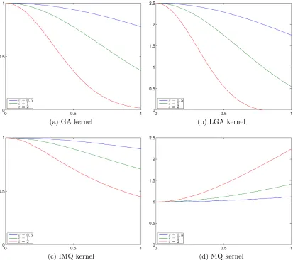
In this study, we focus on radial kernels that feature a shape parameter ε, such as
those in Table 1.1. Decreasing ε increases the flatness of these kernels; this can be
seen in Figure 1.1. The value of ε can have a dramatic effect on the accuracy of the
resulting interpolant. However, choosing an optimal value is still very much an open
question.
(a) GA kernel (b) LGA kernel
(c) IMQ kernel (d) MQ kernel
Figure 1.1: Plots of the radial kernels found in Table 1.1. For each plot, the kernel is ploted for shape parameter values ε= 0.5,1,2.
used ε = 0.8151 d, where d = N1 PN
i=1di such that di is distance between xi and its
nearest neighbor [22]. In another early study, Franke uses ε = 0.8 √
N
D where D is the diameter of the smallest circle containing the interpolation nodes [18] . These
methods try to balance the accuracy of the interpolant and the conditioning of the
interpolation matrix in Eq. 1.2 or 1.5.
Schaback [29] was able to prove that both the accuracy of the RBF interpolant
both be kept low which initially researchers incorrectly thought implied that there
were limits on using small values of the shape parameter ε. The issue with using
small values of ε are that shifts of the radial kernels become less distinct so that the
columns of A look more alike, which leads to ill-conditioning. This is described as
the “uncertainty relation.” However, there is a misconception about this uncertainty
relation. It does not mean that very high accuracies are impossible to achieve with
RBFs, it only means that computing RBF interpolants by solving the linear system
Eq. 1.2 cannot be used to achieve very high accuracies.
The first algorithm to bypass the ill-conditioning problem associated with small
ε was the Contour-Pad´e method [17]. Since then several other methods have been
developed with the most promising being the RBF-QR techniques [8, 14, 16]. The
first RBF-QR method of Fornberg and Pir´et [16] demonstrated that as ε → 0 (the
flat limit) RBF interpolants converge to standard spherical harmonic interpolants for
approximation on the sphere.
We do not use these stable algorithms in this study. The reason is that our
method consists of computing RBF interpolants on a small collection of spherical
caps on the sphere as explained in more detail in Section 2.1. At present, methods
such as Contour-Pad´e and RBF-QR break down for interpolation on these types of
domains. Research is underway to fix this deficiency, and once complete, will be able
to be used directly in our new method.
In this new study, we choose ε so that for the interpolation matrix A, cond (A)≈
tcond, where tcond is a target condition number; this is similar to the first methods
by Hardy and Franke in that it balances accuracy and the condition number. This
technique means thatεincreases as the density of the nodes increases (i.e., the spacing
error” [4, 25], which says that if the condition number is held fixed as the density
of the the node set increases (N → ∞), then there is a point at which the error of
the interpolant cannot get any lower regardless of increasing N. This is explained in
more detail by Maz’ya and Schmidt [25].
1.3
Using RBFs to Solve Partial Differential Equations on
the Sphere
The first attempt to solve Partial Differential Equations (PDEs) using RBFs was by
Kansa [24]. Using the multiquadric as the kernel, Kansa used RBFs in a collocation
approach to solve certain problems from fluid mechanics. Flyer and Wright [11,
12] were the first to apply RBFs to hyperbolic PDEs on the surface of the sphere,
including the transport equation and full nonlinear shallow water wave equations. We
describe their method for the transport equation since it is similar to the new method
we have developed.
The transport of a quantity h on the sphere with no external forcing or body
forces is governed by the hyperbolic PDE
∂
∂th(x, t) =−u(x, t)·(P∇h(x, t)),x∈S 2
, t >0 (1.6)
where u(x, t) is some incompressible velocity field tangent to the sphere and P∇
represents the surface gradient operator on the sphere. This operator is written with
respect to Cartesian coordinates to avoid singularities that would occur in any two
dimensional parameterization of the sphere, such as spherical coordinates. Thus, ∇
operator that projects vectors in R3 to vectors tangent to the sphere.
The specific construction of P is as follows: let x ∈ S2 and u ∈
R3. If n is the
surface normal ofS2 at xthen nnTu gives the projection of u ontox and u−nnTu gives the projection of u onto the plane tangent to the sphere at x. The surface
normal to S2 atx isx. Thus, if x= (x, y, z), then P can be defined as:
P =I−xxT =
(1−x2) −xy −xz
−xy (1−y2) −yz
−xz −yz (1−z2)
= pT x pT y pTz
. (1.7)
The standard gradient ∇ can now be constrained to the surface of the sphere:
P∇=
px· ∇ py · ∇ pz· ∇
. (1.8)
To solve Eq. 1.6 with the global RBF method, the ∇ operator is first discretized
using the RBF interpolant form Eq. 1.1. LetX ={xi}Ni=1 ⊂S2 be the nodes at which
the solution to the PDE will be computed. The partial derivative of Eq. 1.1 with
respect to xis
∂
∂xs(x) =
N
X
i=1 ci
∂
∂xφ(kx−xik) (1.9)
where the coefficients {ci}Ni=1 are determined by the system Eq. 1.2 such that c = A−1f. Sinces(x) approximates a function f(x), the partial derivative atx=xj can be approximated as
∂ ∂xf(x)
x=xj ≈
∂ ∂xs(x)
x=xj =
N
X
i=1 ci
∂
∂xφ(kx−xik)
By defining a matrix Bx such thatBx
ij = ∂x∂φ(kxj −xik), then the partial derivative of f at all nodes in X can be approximated as:
∂ ∂xf
X ≈
∂ ∂xs
X =Bxc=BxA
−1
| {z }
Dx
f (1.11)
where we have used the shorthand notation g
X = [g(x1), g(x2), . . . , g(xn)]
T. Here
Dx is referred to as a differentiation matrix. Matrices that compute the partial derivatives with respect toy and z of Eq. 1.1 at X (Dy and Dz) can be constructed in a similar way.
Let xi = (xi, yi, zi) ∈ X and let x = [x1, x2, . . . , xN]T, y = [y1, y2, . . . , yN]T, and
z = [z1, z2, . . . , zN]T. Now each component of P∇ can be approximated at X using the differentiation matrices Dx, Dy, Dz as follows:
Gx := diag (1−x◦x)Dx+ diag −x◦yDy + diag (−x◦z)Dz Gy := diag −x◦yDx+ diag 1−y◦yDy + diag −y◦zDz Gz := diag (−x◦z)Dx+ diag −y◦z
Dy + diag (1−z◦z)Dz
(1.12)
where ◦ is the Hadamard product, or element wise multiplication operator. Finally,
letting u, v, w represents the components of u sampled at X, a linear operator D
can be constructed to approximate the differential operator on the right hand side of
Eq. 1.6 as follows:
D= diag(u)Gx+ diag(v)Gy+ diag(w)Gz. (1.13)
This process would be similar if the interpolant from Eq. 1.4 was used, where the
The differentiation matrix D is then used in a method-of-lines (MOL) approach
for approximating the solution to Eq. 1.6. In this method, the initial conditionh(x,0)
at X, h0 = h[(x1,0), h(x2,0), . . . , h(xn,0)]T and the spatial derivatives in the RHS of Eq. 1.6 are replaced by D, leading to the semi-discrete system:
d
dth=−Dh. (1.14)
This system can then be advanced in time using a standard ODE solver such as the
classical fourth-order Runge-Kutta method (RK4).
The global RBF method has several desirable features. First, since this method
uses RBF interpolation it does not depend on a mesh (or it’s mesh-free). Thus,
the nodes can be distributed in an optimal way to “uniformly” cover the sphere.
Additionally, the method uses Cartesian coordinates and is therefore free of coordinate
singularities. Lastly, this method compares favorably to other spectral methods in
terms of accuracy per degree-of-freedom and time step that can be used for stable
time integration [11, 12].
There are, however, limitations with this method. First, the time complexity of
constructing the matrixDin Eq. 1.13 isO(N3), whereN is the number of nodes. The
space complexity ofDisO(N2) since D is dense. Finally, each matrix multiplication
with D required for time integration of Eq. 1.14 has a time complexity of O(N2).
Thus, this method is not practical for large N as is required in realistic simulations
1.4
Overview of Thesis
In this thesis, we introduce the Radial Basis Function Partition of Unity Method
(RBF-PUM) to address the computational complexity issues with global RBF method
[11, 12]. The basic idea is to first distribute a set of nodes quasi-uniformly over the
surface of the sphere as done in the global method. Next, the surface of the sphere
is partitioned into overlapping spherical caps so that each cap contains roughly the
same number ofnnodes. All spatial derivatives of the PDE are approximated locally
within the caps using the standard RBF method. The approximations from each cap
are then aggregated into one global approximation of the spatial derivatives using an
appropriate weight function in the PUM.
The time-complexity associated with constructing a differentiation matrix (1.13)
with this new method is reduced to O(NlogN), while each multiplication of Dby a
vector has a time complexity of O(N). Thus, the computational cost scales linearly
withN for each time-step of the time integration. The accuracy of this new method no
longer exhibits an exponential convergence rate, but it still provides very high (near
exponential) accuracy for smooth initial conditions. Additionally, the new method
remains mesh-free, and free of any coordinate singularities.
In Chapter 2, the RBF-PUM method is introduced. Section 2.1 gives details on the
construction of the RBF-PUM method. In Section 2.2, we show how the RBF-PUM
can be parameterized with respect to the number of nodes N, number of nodes
per spherical cap n, and the average number of spherical caps a node belongs to q.
Details about computing the RBF-PUM matrices are given in Section 2.3. Section 2.4
gives details about the time complexity of constructing the RBF-PUM differentiation
Section 2.6, we show how the RBF-PUM can be stabilized for time-integration.
In Chapter 3, we test the RBF-PUM method on a set of standard test problems
from the literature. We analyze results from the cosine bell test [33], deformational
flow test [28] with non-smooth cosine bell and Gaussian bell initial conditions and
finally stationary vortex roll-up test [27]. These numerical results demonstrate that
the new method exhibits near exponential convergence for smooth solutions. Lastly,
we provide analysis based on the numerical data.
CHAPTER 2
RBF PARTITION OF UNITY METHOD (RBF-PUM)
In the RBF-PUM method, local interpolants are constructed on subsets (or patches)
ofS2and the combined using weight functions{w
i}that form a partition of unity. The method was first introduced by Cavoretto and DeRossi in [5] for interpolation
prob-lems on the sphere. Below we present the method first as an interpolation technique
then describe how it can be used to approximate spatial derivatives on the sphere.
We start the discussion with a description of how the sphere is partitioned and the
weight functions are constructed. We follow this by showing how the differentiation
matrix D from Section 1.3 can be constructed using the RBF-PUM method. Next,
we analyze the time complexity of constructing D and its sparsity. Finally, we show
how D can be stabilized via hyperviscosity.
2.1
Constructing the RBF Partition of Unity Interpolant
A partition of unity can be defined as follows [31]:
Definition 1. A partition of unity on a topological space S is a family {wi} of
continuous functions
wi :S→R+
1. {suppwi} is a locally finite covering of S,
2. ∀x∈S :P
i
wi(x) = 1.
In our application, S is the unit sphere S2 and the details on constructing the
partition of unity are as follows:
Let X ={xi}Ni=1 be a set of scattered nodes on S2 and Ω1,Ω2, . . . ,ΩM be a set of distinct spherical caps on S2 such that
1. M
S
i=0
Ωi =S2 i.e. the caps cover the surface of sphere; and
2. Each cap contains at least one node in X.
We refer to the spherical caps as patches. For each patch Ωk, define ξk ∈ S2 as the center of patch Ωk and ρk as the radius of the patch, measured as the Euclidean distance fromξk. For each patch, we define a continuous compactly supported weight function ψk on Ωk as follows:
ψk(x) =ψ
k
x−ξkk
ρk
, (2.1)
where ψ has compact support over the interval [0,1). In this study, we use the cubic
B-spline
ψ(r) =
2
3 + 4 (r−1)r
2 if 0≤r < 1 2,
−4
3(r−1) 3
if 12 < r≤1,
0 if r >1.
which has two continuous derivatives on [0,1]. Each ψk has compact support on Ωk. We define wk as follows:
wk(x) = ψk(x) M
P
i=0 ψi(x)
. (2.3)
Since each wk has compact support on Ωk, and ∀x∈S2
M
P
k=0
wk(x)≡1, {wk} forms a partition of unity onS2.
These weight functions are used in the RBF-PUM interpolant as follows. For
each Ωk, define Xk as the set of x∈ X such that x∈Ωk. Let sk be the global RBF interpolant from Section 1.1, either Eq. 1.1 or 1.3, defined on the nodesXk. The RBF partition of unity interpolant is given
s(x) = M
X
k=0
wk(x)sk(x). (2.4)
Suppose {fi}Ni=1 ⊂ R is data sampled at X, and let xi ∈ X. We know from Section 1.1 that if x ∈ Ωk, then sk(xi) = fi . By construction, if xi 6∈ Ωk, then
wk(xi) = 0 (since the weight functions have compact support over their associated patches). Thus,
M
X
i=0
wk(xi) =
X
Ωk3xi
wk(xi)≡1, (2.5)
which implies
s(xi) = M
X
i=0
wk(xi)sk(xi) =
X
Ωk3xi
wk(xi)fi =fi
X
Ωk3xi
wk(xi) = fi, (2.6)
2.2
Choosing the Nodes and Patches
Since the interpolant of (2.4) does not require the nodes X to be on a grid or mesh,
we are free to choose them however we wish for our application. In this study, we
focus on node sets that are quasi-uniformly distributed on the sphere so as to get
near optimal resolution of the entire sphere. Since there exists no equidistant node
sets on the sphere where the number of nodes is greater than 20, there are several
techniques for generating quasi-uniform points on the sphere. We use the maximum
determinant (MD) method for generating these nodes [35]. The MD method choses
the nodes in such a way that the determinant of an interpolating matrix that depends
on spherical harmonics is maximized. These node sets have been generated for various
number of nodes and can be freely downloaded from [30]. For patch centers, we use
the minimum energy (ME) points. These node sets are computed by minimizing the
Reisz energy (with a power of 2) of the node set over the sphere [21]. For information
on how we generated the patch centers, see Appendix A.
Given a MD node set, we determine the patches based on two criteria:
1. the approximate number of nodes each patch will contain,
2. the average number of patches a node belongs to.
Suppose there are N nodes and we want approximately n nodes per patch. Because
the nodes are quasi-uniformly distributed, we can expect the area per node ratio over
the entire sphere to roughly equal the area per node ratio on the patch. If ρk is the radius of patch Ωk, then this area relationship gives
4π
N ≈
πρ2
k
Thus, we can approximate ρk as
ρk ≈2
r
n
N. (2.8)
Since the patch centers are also quasi-uniformly distributed, all patch radii can be
chosen the same way, i.e ρk =ρ, for all k.
For each node xk, let qk be the number of patches xk belongs to. This can be used as a measure of overlap in that if the values of {qi}Ni=1 are high, there is more
overlap between the patches. Considering that all patches have radius ρ, the number
of patches thatxk belongs to is the same as the number of patch centers in a spherical cap centered at xk with radius ρ. We choose q to represent the average of {qi}Ni=1.
Suppose there are M patch centers. Since these are quasi-uniformly distributed we
can expect that the area per center ratio for the sphere is approximately equal to the
area per center ratio for the spherical cap centered at any node, i.e.
4π
M ≈
πρ2
q . (2.9)
We can thus approximate M as
M ≈
4q ρ2
≈
qN n
. (2.10)
We numerically verify in Appendix B that when we chose M andρwith (2.8) and
(2.10), that the actual number of number nodes per patch and average number of
patches a node belongs to corresponds very closely with there respective parameters
2.3
Approximating the Surface Gradient Operators
We use the RBF-PUM in a similar way to the global RBF method [11, 12] discussed
in Section 1.3 to discretize the spatial derivative operators associated with the right
hand side of Eq. 1.6. The first thing that needs to be considered is how to construct
the discrete operators for the components of the surface gradient. Interpolation in the
RBF-PUM occurs at two levels: globally and locally. Locally we use the direct RBF
method for each of the patches where globally we use the RBF-PUM on the sphere
itself. The partial derivative of the RBF-PUM interpolant in Eq 2.4 with respect to
x is
∂
∂xs(x) =
M
X
k=1
wk(x)
∂
∂xsk(x) +sk(x) ∂
∂xwk(x)
. (2.11)
The equation for the partial derivative of the weight with respect to x is
∂
∂xwk(x) =
∂
∂xψk(x) m
P
i=1
ψi(x)−ψk(x) m
P
i=1
∂ ∂xψi(x)
m
P
i=1 ψi(x)
2 . (2.12)
Since wk(x) has compact support on Ωk, both sk(x) and ∂x∂ sk(x) only need to be computed for x ∈ Xk. We compute ∂x∂ sk
Xk similarly to the direct RBF method
described in Section 1.3 with a differentiation matrix Dx k. Given that for all k, ∂x∂ sk
Xk = D
x kf
Xk,sk
Xk =f
Xk, and wk(x) is independent
of f, it is possible to construct a differentiation matrixDx such that
∂ ∂xf X ≈ ∂ ∂xs
X =D
Differentiation matricesDy,Dzcan similarly be constructed for the spatial derivatives
y and z, respectively. The components of the projected gradient Gx, Gy, and Gz
from (1.12) can then be approximated in a similar fashion, but by using the
RBF-PUM differentiation matrices instead. The differentiation matrixDfor the advection
operator from Eq. 1.13 can then be computed by replacing the components of the
projected gradient from the global RBF method with that of the RBF-PUM. This
new Dcan be used to solve the PDE (1.6) via the method of lines using the classical
Runge-Kutta-Method (with some minor modification as discussed in Section 2.6).
2.4
Computational Complexity of Constructing RBF-PUM
Differentiation Matrices
One advantage that the RBF-PUM has over the direct RBF method is that the
com-putational complexity for construction is more manageable than the global method.
To analyze this complexity, we start with a set of quasi-uniformly distributed nodes
X ={xi}Ni=1, a set of quasi-uniformly distributed patch centers{ξk}Mk=1, and a radius
for all patches ρ. These are chosen with parameters N, n, and q as specified in
Section 2.2.
Suppose thatnandqare fixed, and letnk be the number of nodes in patch Ωk and
qi be the number of patchesxi belongs to. Even thoughn andq are fixed, it needs to be shown how nk and qi behave asymptotically for large N. We can use Proposition 14.1 from [32], which states that there exists constants c1 and c2 such that
c1N−1/3 ≤hX,S2 ≤c2N
−1/3
where hX,S2 is the fill distance, or the largest radius r such that a ball of this radius
centered at xi (i.e., B(xi, r)) contains no other node. The proposition does this by considering the volume of spheres centered atxi. If we take advantage of the topology of S2, we can instead use spherical caps to reach this conclusion:
c1N−1/2 ≤hX,S2 ≤c2N
−1/2. (2.15)
Corollary 14.2 from [32] argues using Proposition 14.1 that for a cube whose side
is equal to 2cN−1/3, the number of number of nodes in that cube is bounded by
the constant independent of N regardless of its location; it does this by considering
the cube enclosed by a sphere. If we instead use spherical caps, a similar proof can
be made to show that if the radius of a spherical cap is bounded by cN−1/2, then
the number of nodes in the spherical cap is bound by a constant independent of N
(regardless of its location on the sphere).
From Section 2.2, we have that ρ is chosen so that ρ = 2pNn. Thus, if n is fixed, there must exist a constant C independent of N such that for all patches Ωk,
nk ≤ C. Considering that M linearly depends on N by construction (2.10), it can be inferred that there exists a constant c such that ρ ≤ c
q
1
M. Thus, if we consider that if there were spherical caps centered at xi (where qi would be the number of centers in the caps), a similar argument can be made that there exist a constant
K independent of M such that qi < K. Since M depends on N though, it must be the case that K is independent of N as well. Our numerical evidence strongly
suggests thatn ≈ 1
M
PM
i=1ni andq ≈ 1
N
PN
i=1qi so that we can arguenk =O(n) and qk=O(q).
nodes that belong to it. This can be done efficiently by building a kd-tree using the
node points [32]. The time complexity of constructing the tree is O(NlogN), while
the space complexity is O(N). The time to find the nodes that are ρ away from
the patch center ξk isO(logN), so that the time to determine this for all patches is
O(MlogN). Considering thatM =O(N) by construction (there will never be more
patches than nodes), we have that the computational cost of building the kd-tree and
determining the patches to be O(NlogN).
The differentiation matrices Dx k, D
y
k, and Dzk must be computed for each patch Ωk. The computational cost for constructing the differentiation matrices for Ωk is
O(n3), making the total time for all patches O(M n3). From Eq. 2.10, it can be
inferred that M =O qNn so that we have O(N qn2). Computing these matrices is embarrassingly parallel because computing the differentiation matrices for patch Ωk requires no information from any other patch. Next, the partition of unity weight
functions and partial derivative values have to be computed. The time complexity
for calculating the partition of unity weights for xi is O(q), making the complexity
O(N q) for all the nodes.
Finally, we have to assemble the RBF-PUM differentiation matrices Dx,Dy and
Dz. Let’s consider computing the ith column of Dx, which is the vector of values
fi would be multiplied with for the RBF-PUM partial derivative with respect to x for all nodes. Looking at Eq. 2.11, the only Dx
k that would be used for this column are the Dx
k such that xi ∈ Ωk; we would also have to use ∂x∂ wk(x) for that patches xi belongs to. Thus, the number of computations needed to compute this column would be O(qn+q) = O(qn). This makes the computational cost of assembling Dx
evaluating the partition of unity weight functions and partial derivative values, and
constructing the differentiation matrices for the RBF-PUM is O(N qn2). The total
computational cost for construction is therefore O(N qn2+NlogN). Since n N
and q = O(1), this is a significant savings over the global method, which has a cost
of O(N3).
2.5
Sparsity of the RBF-PUM Differentation Matrices
It can be shown that the RBF-PUM differentiation matrices are significantly more
sparse than the differentiation matrices from the global RBF method in Section 1.3
(which are in fact dense). In this section, we make estimates on the sparsity of the
RBF-PUM differentiation matrices and compare these to the values seen in practice.
Let’s consider Dxij, which is the value we multiply fi by to compute (2.11) at xj. From Section 2.2, it is clear thatwk(xj) = ∂x∂ wk(xj) = 0 if and only ifxj 6∈Ωk. Also if fi is used to compute sk(xj) or ∂x∂ sk(xj), then xi is in Ωk. Thus, if there is no patch Ωk such that xi and xj both belong to it, then Dij = 0. This means for the
ith column of Dx, the number of non zeros is bounded by the number of nodes that are also in a patch with xi, or
S
Xk3xiXk
. This is similarly true forDy and Dz. Let
nnz be the number of non-zero entries in a given RBF-PUM differentiation matrix.
Then, nnz ≤ N X i=0 [
Xk3xi
Xk ≤ N X i=0 X
Xk3xi
nk=O(N nq). (2.16)
Since nN and q =O(1), the matrices have nice sparsity properties.
In part (a) of Tables 2.1-2.3, we display the ratio of the actual nnz of the
RBF-PUM differentiation matrices to our estimate N nq for different n and N with
constant in front of N nq being less than one. Additionally, this estimate decreases
with increasing q. In part (b) of Tables 2.1-2.3, we display the percent full of the
computed RBF-PUM differentiation matrices confirming the nice sparsity properties
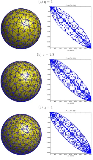
of those matrices. In Figure 2.1, we illustrate how the patches and sparsity of the
differentiation matrices change with increasing q for the case ofN = 4096 nodes and
n= 100.
Table 2.1: Ratio of number of non zeros in a differentiation matrix compared to our estimate and percent full the differentiation matrices are with q=3.
(a) Ratio
nN 4096 6400 9216 12544 16384 20736 25600
100 0.71 0.71 0.72 0.72 0.72 0.72 0.72
144 0.71 0.71 0.72 0.72 0.72 0.72 0.72
196 0.71 0.71 0.71 0.72 0.72 0.72 0.72
256 0.71 0.71 0.71 0.71 0.71 0.72 0.72
(b) Percent Full
nN 4096 6400 9216 12544 16384 20736 25600
Table 2.2: Ratio of number of non zeros in a differentiation matrix compared to our estimate and percent full the differentiation matrices are with q=3.5.
(a) Ratio
nN 4096 6400 9216 12544 16384 20736 25600
100 0.65 0.65 0.65 0.65 0.66 0.65 0.66
144 0.65 0.65 0.65 0.65 0.65 0.65 0.66
196 0.65 0.65 0.65 0.65 0.65 0.65 0.65
256 0.64 0.65 0.65 0.65 0.65 0.65 0.65
(b) Percent Full
nN 4096 6400 9216 12544 16384 20736 25600
100 5.56% 3.57% 2.48% 1.82% 1.40% 1.11% 0.90% 144 7.99% 5.14% 3.58% 2.62% 2.01% 1.59% 1.29% 196 10.85% 6.99% 4.86% 3.57% 2.74% 2.16% 1.75% 256 14.03% 9.09% 6.32% 4.66% 3.57% 2.82% 2.29%
Table 2.3: Ratio of number of non zeros in a differentiation matrix compared to our estimate and percent full the differentiation matrices are with q=4.
(a) Ratio
nN 4096 6400 9216 12544 16384 20736 25600
100 0.60 0.60 0.60 0.60 0.60 0.60 0.60
144 0.60 0.60 0.60 0.60 0.60 0.60 0.60
196 0.59 0.60 0.60 0.60 0.60 0.60 0.60
256 0.59 0.60 0.60 0.60 0.60 0.60 0.60
(b) Percent Full
nN 4096 6400 9216 12544 16384 20736 25600
Figure 2.1: Illustration of the nodes and patches used in the RBF-PUM for increasing
q with parametersN = 4096 and n= 100. Here the black solid circles reperesent the nodes, blue spherical caps represent the patches, and the red solid circles represent the centers of the patches. The sparsity of the corresponding differentiation matrices is also shown for eachq.
(a) q = 3
(b) q = 3.5
2.6
Stabilization via Hyperviscosity
Our semi-discrete or method-of-lines formulation of the transport equation (1.6) takes
the form
d
dth=−Dh, (2.17)
where D represents the RBF-PUM discretization of the the advection operator u·
(P∇) (see Eq. (1.13)). A necessary condition for stability of this formulation is that
the eigenvalues of −D must be in the stability domain of the ODE solver used for
advancing the system in time. At the very least, this means that all the eigenvalues
of −D must be in the left half plane. Since the advection operator contains no
natural dissipation term, this is an extraordinary condition to put on the numerical
discretization scheme. The RBF-PUM method does not satisfy this requirement and,
like many methods for solving hyperbolic PDEs on non-rectangular grids, a numerical
“stabilization” term needs to be included to shift the eigenvalues to the left half plane.
A common approach for stabilizing high-order finite-difference and collocation
methods is to include a hyperviscosity dissipation term in Eq. 2.17:
d
dth=−(D−µH)h, (2.18)
whereH is the numerical discretization of the hyperviscosity term ∆p,p∈
N, andµis
a weighting constant. The goal of this approach is to pickpandµto stabilize the time
integration of the numerical scheme without causing a deterioration in the accuracy
of the spatial discretization. Typically, the higher-order the method, the larger the
value of p is used so that the dissipation term only damps the highest frequency
other RBF methods [2, 10, 15].
We adopt a similar approach to stabilizing the RBF-PUM method, however,
instead of using a hyperviscosity term of the form ∆p, we follow the approach proposed in [15] for stabilizing the global RBF method for the transport equation discussed in
Section 1.3. In this approach, one uses the inverse of the RBF interpolation matrix
A from Eq. 1.2 as H in Eq. 2.18. As argued in [15], the matrix A−1 acts like an
approximation to a high power of the Laplace-Beltrami operator on the sphere. The
issue with using this method directly is that it would require computing A−1 based
on the whole set of nodes in X, which would require a computational cost of O(N3).
We instead construct H by first computing inverses of the interpolation matrices on
each of theM patches,A−k1, k= 1, . . . , M. We then combine these inverses using the partition of unity weight functions to get a sparse approximation to the global version
of the hyperviscosity matrix A−1. The computational complexity of constructing H
is similar to that of constructing the RBF-PUM differentiation matrices Dx,Dy, and
Dz, and the sparsity properties of H are identical to these matrices.
To illustrate the effects of the hyperviscosity term, we consider the advection
operator corresponding to the velocity field u =
0 z −y
T
, which corresponds to
solid body rotation of the sphere (this is also the first test case we consider in Chapter
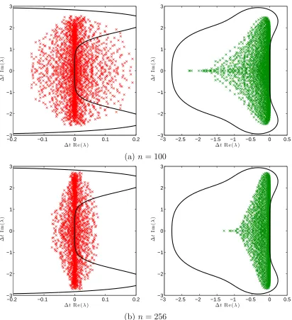
3). In the left column of Figure 2.2, we display the eigenvalues of the RBF-PUM
differentiation matrix −D for this advection operator using N = 4096 nodes and
two values of n. The stability domain of the standard fourth order Runge-Kutta
(RK4) method is also plotted in this figure and the eigenvalues have been scaled by
∆t = 2π/1600. We can see that the eigenvalues for both values of n are scattered
into the left half-plane and outside the stability domain of RK4, so that stable time
−0.2 −0.1 0 0.1 0.2 −3 −2 −1 0 1 2 3
∆tR e (λ)
∆ t Im ( λ )
−3 −2.5 −2 −1.5 −1 −0.5 0 0.5 −3 −2 −1 0 1 2 3
∆tR e (λ)
∆ t Im ( λ )
(a) n= 100
−0.2 −0.1 0 0.1 0.2 −3 −2 −1 0 1 2 3
∆tR e (λ)
∆ t Im ( λ )
−3 −2.5 −2 −1.5 −1 −0.5 0 0.5 −3 −2 −1 0 1 2 3
∆tR e (λ)
∆ t Im ( λ )
(b) n = 256
Figure 2.2: Eigenvalues of the RBF-PUM differentiation matrix for the advection operator corresponding to solid body rotation for the case of N = 4096 nodes, a target condition number of tcone = 1012, and q = 4. The left column shows the
eigenvalues of the stabilized differentiation matrix −(D−µH). We see that for both
values ofn, all eigenvalues have been shifted to the left-half plane and are contained in
the stability domain of RK4. Thus, this version is suitable for stable time integration.
In the next chapter, we see that this hyperviscosity stabilization does not have a
CHAPTER 3
NUMERICAL RESULTS
In this chapter, we apply the RBF-PUM method to several standard benchmark
problems in the literature to analyze its performance. All tests are for the transport
equation:
∂
∂th(x, t) +u(x, t)·P∇h(x, t) = 0, (3.1)
where P∇ is the surface gradient and u is tangent to the sphere. In some of these
tests, u can be defined by a stream function ψ(x, t)
u=x× ∇ψ (3.2)
where possible, we will state these tests in terms of ψ.
For all of the tests, we present results for two kernels: the Gaussian (GA) and
inverse multiquadric (IMQ) listed in Table 1.1. We compute solutions for increasing
values of N and n and analyze the convergence of the method. We test with values
N = 4096, 6400, 9216, 12544, 16384, 20736, and 25600; n = 100, 144, 196, 256; and
q = 4. The errors between the approximate and true solutions are computed using
the l2 and l∞ norms. The convergence is measured as a function of
√
N since the
spacing between the nodes decreases asymptotically like 1/√N, which follows from
the results for two target condition numberstcond to examine the effect of saturation
errors. For each test, the hyperviscosity parameter µ is fixed for all N and n. The
standard fourth-order Runge-Kutta method (RK4) is used for the time integration
with the time step ∆t fixed (and not optimized) for each test. Finally, all tests were
performed using MATLAB 2012b.
3.1
Cosine Bell Test
As a first test problem we will consider the standard Test Case 1 from Williamson
et al. [33]. For this problem, the initial height field is the following cosine bell:
h(x) =
1
2(1 + cos (3πr(x))) r(x)< 1 3
0 r(x)≥ 1
3
(3.3)
where r(x) = arccos(x), and x = (x, y, z). This initial condition has a jump in the
second derivative at the support of the bell, which makes the test susceptible to both
diffusive and dispersive errors. The stream function is time-independent and is given
by
ψ(x) = xsin (α)−zcos (α) (3.4)
This stream function results in solid body rotation at an angle of α with respect to
the equator. In our test, we use the standard value of α = π2, which corresponds to the flow over the poles. The test is run up to time t = 2π, which corresponds to one
full rotation at which point the solution is equal to Eq. 3.3. The error between the
numerical and true solution is then computed.
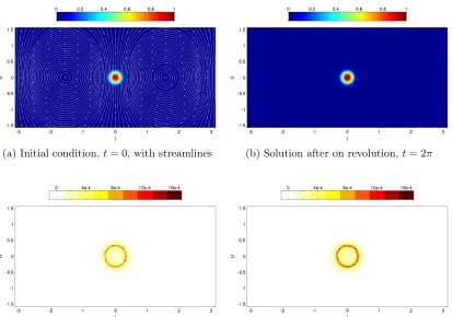
these solutions are the same as dictated by the stream function (3.4). Figure 3.1c
shows the magnitude of the error after one revolution and we can see that errors are
concentrated near the discontinuities of the cosine bell. It can be seen in Figure 3.1d
that the errors are still concentrated around the edges of the bell even after 10
revolutions. Thus, the scheme is performing quite well with respect to diffusive and
dispersive errors.
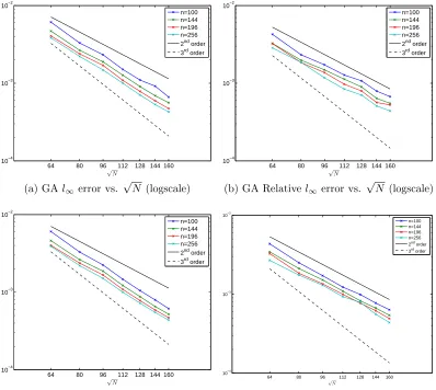
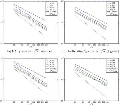
In Figures 3.2 and 3.3, we plot the relative errors of the method for target condition
numbers oftcond = 1014andtcond = 1012. The figures show that the method producing
approximately second order convergence for all nand both target condition numbers.
This is the maximum convergence possible since the initial condition has a jump in
its second derivative. As expected, increasing n decreases the error. Finally, we see
that decreasing the target condition number does not have a significant effect on the
(a) Initial condition, t= 0, with streamlines (b) Solution after on revolution,t= 2π
(c) Magnitude of the error after one revolution (d) Magnitude of the error after ten revolutions
64 80 96 112 128 144 160 10−4 10−3 10−2 √ N n=100 n=144 n=196 n=256 2nd order 3rd order
(a) GAl∞error vs. √
N (logscale)
64 80 96 112 128 144 160
10−4 10−3 10−2 √ N n=100 n=144 n=196 n=256 2nd order 3rd order
(b) GA Relativel∞error vs. √
N (logscale)
64 80 96 112 128 144 160
10−4 10−3 10−2 √ N n=100 n=144 n=196 n=256 2nd order 3rd order
(c) IMQ Relativel2 error vs. √
N(logscale)
64 80 96 112 128 144 160
10−4 10−3 10−2 √ N n=100 n=144 n=196 n=256 2nd order 3rd order
(d) IMQ Relativel∞error vs. √
N (logscale)
Figure 3.2: Convergence plots of the cosine bell test using the GA and IMQ kernels as a function of N and n, ∆t = 2π/1600, and tcond = 1014; for the GA kernel test
64 80 96 112 128 144 160 10−4 10−3 10−2 √ N n=100 n=144 n=196 n=256 2nd order 3rd order
(a) GAl2 error vs. √
N (logscale)
64 80 96 112 128 144 160
10−4 10−3 10−2 √ N n=100 n=144 n=196 n=256 2nd order 3rd order
(b) GA Relativel∞error vs. √
N (logscale)
64 80 96 112 128 144 160
10−4 10−3 10−2 √ N n=100 n=144 n=196 n=256 2nd order 3rd order
(c) IMQ Relativel2 error vs. √
N(logscale)
64 80 96 112 128 144 160
10−4 10−3 10−2 √ N n=100 n=144 n=196 n=256 2nd order 3rd order
(d) IMQ Relativel∞error vs. √
N (logscale)
3.2
Deformational Flow Tests
The next test is from Nair and Lauritzen [28]. The stream function for the flow is
ψ(x(t)) = 2 [y(t)]2cos
πt
5 − 2π
5 z(t)
,
x(t) =
cos
λ− 2πt
5
cosθ,sin
λ− 2πt
5
,sinθ
.
(3.5)
This results in a velocity field that is a combination of solid-body rotation with a
deformational component. There are two initial conditions considered. First is the
non-smooth cosine bells, similar to the previous test:
h(x) = 0.1 + 0.9 (h1(x) +h2(x)) , where
hi(x) =
1
2(1 + cos (2πri(x))), ri(x)< 1 2,
0, ri(x)≥ 12,
ri(x) = arccos xTxi
,
x1 =
√
3 2 ,
1 2,0
!
,
x2 =
√
3 2 ,−
1 2,0
!
.
(3.6)
The second initial condition is the smooth Gaussian bells:
h(x) = 0.95(exp(−(4kx−x1k)2) + exp(−4(kx−x2k)). (3.7)
This test advects the initial condition around the sphere while at the same time
deforming them. At time t = 2.5, the flow field reverses and the initial condition
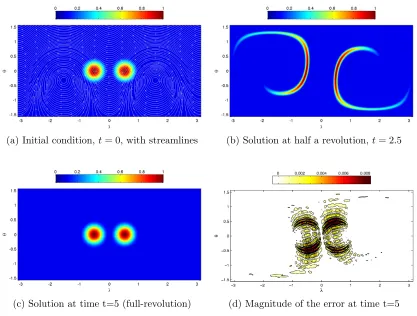
Figures 3.4a, 3.4b, and 3.4c show the solution at the start, half a revolution,
and one revolution respectively for the test using the non-smooth cosine bells. In
Figure 3.4d, we see that the errors are most significant near the location of the
discontinuity of the cosine bells. Figures 3.5 and 3.6 show that the convergence for
both kernels appears to be second order. This is again related to the smoothness of
the initial conditions. As with the cosine bell test in Section 3.1, there appears to
be no significant change in errors when the target condition number is decreased and
when the GA or IMQ kernels are used.
Figures 3.7a, 3.7b, and 3.7c show the solution at the start, half a revolution, and
one revolution respectively but for the smooth Gaussian bells. The magnitude of the
error Figure 3.7d is much lower than that of Figure 3.4d, but is still largely clustered
around the location of the bells. The errors are plotted in Figures 3.5 and 3.6 on a
log-linear scale instead of a log-log scale. The straight line behavior indicates that the
errors appear to decrease at an exponential rate until a point where they level off. The
point where they level off decreases with increasing condition number in line with the
theory presented by Maz’ya and Schmidt [25]. The results show that saturation errors
set in at roughly the same point for both the GA and IMQ kernels. However, even
with saturation error, the method is still providing very accurate results compared to
(a) Initial condition, t= 0, with streamlines (b) Solution at half a revolution,t= 2.5
(c) Solution at time t=5 (full-revolution) (d) Magnitude of the error at time t=5
Figure 3.4: Plots of the solution and error using non-smooth cosine bells with the GA kernel for N = 20736, n= 100, ∆t = 5/2400, µ= 10−10,t
64 80 96 112 128 144 160 10−3 10−2 10−1 √ N n=100 n=144 n=196 n=256 2nd order 3rd order
(a) GA Relativel2 error vs. √
N(logscale)
64 80 96 112 128 144 160
10−3 10−2 10−1 √ N n=100 n=144 n=196 n=256 2nd order 3rd order
(b) GA Relativel∞error vs. √
N (logscale)
64 80 96 112 128 144 160
10−3 10−2 10−1 √ N n=100 n=144 n=196 n=256 2nd order 3rd order
(c) IMQ Relativel2 error vs. √
N(logscale)
64 80 96 112 128 144 160
10−3 10−2 10−1 √ N n=100 n=144 n=196 n=256 2nd order 3rd order
(d) IMQ Relativel∞error vs. √
N (logscale)
(a) Initial condition, t= 0, with streamlines (b) Solution at half a revolution,t= 2.5
(c) Solution at time t=5 (full-revolution) (d) Magnitude of the error at time t=5
64 80 96 112 128 144 160 10−6 10−5 10−4 10−3 10−2 10−1 √ N n=100 n=144 n=196 n=256
(a) GA Relative l2 error vs. √
N(loglinear scale)
64 80 96 112 128 144 160
10−6 10−5 10−4 10−3 10−2 10−1 √ N n=100 n=144 n=196 n=256
(b) GA Relative l∞ error vs. √
N (loglinear scale)
64 80 96 112 128 144 160
10−6 10−5 10−4 10−3 10−2 10−1 √ N n=100 n=144 n=196 n=256
(c) IMQ Relative l2 error vs. √
N(loglinear scale)
64 80 96 112 128 144 160
10−6 10−5 10−4 10−3 10−2 10−1 √ N n=100 n=144 n=196 n=256
(d) IMQ Relative l∞ error vs. √
N (loglinear scale)
3.3
Stationary Vortex Roll-Up
In this test, two vortices are generated at the north and south poles of the sphere,
providing an idealized model for cyclogenisis. This test was first introduced in [26].
The velocity field is given by
u=ω(θ) cosθ,
v = 0
(3.8)
with
ω(θ) =
3√3 2 sech
2(ρ(θ)) tanh (ρ(θ)) ρ(θ)6= 0
0 ρ(θ) = 0
(3.9)
where ρ(θ) = ρ0cos (θ) and ρ0 is a parameter controlling the radial extent of the
vortex; in this test ρ0 = 3. The analytical solution to this PDE is given by:
h(λ, θ, t) = 1−tanh
ρ(θ)
5 sin (λ−ω(θ)t)
. (3.10)
The initial condition is given by Eq. 3.10 at t = 0. The test calls for computing the
errors in the numerical solution at time t= 3 using the analytical solution (3.10).
Numerical solutions for this test problem are plotted at times t = 3, t = 6 and
t = 9 in Figures 3.10a, 3.10b, and 3.10c, respectively. The magnitude of the errors
at these times are plotted in Figures 3.10d, 3.10e, and 3.10f. We see that as time
increases, the errors become more and more concentrated at the centers of the vortices
(where the gradients are the highest).
Figure 3.11 and 3.12 show the relative errors in the solution for the two target
the results indicate the method is giving between 7th and 8th order convergence. As
in the previous tests with the Gaussian bell, we do see that saturation errors again
show up for increasing N. Increasing the condition number does allow convergence
to proceed further with increasing N, but eventually saturation does appear. The
results also show that the IMQ kernel is less susceptible to saturation errors than the
GA kernel for this test, as the IMQ kernel is able to achieve a relative error at least
one order of magnitude lower than the GA kernel. Again even with saturation error,
the method is still providing very accurate results compared to other methods that
use a similar number of degrees of freedom [27].
(a) Solution att= 3 (b) Solution att= 6 (c) Solution at t= 9
(d) Magnitude of the error at timet= 3
(e) Magnitude of the error at timet= 6
(f) Magnitude of the error at timet= 9
Figure 3.10: Plots of the solution and error of the stationary vortex roll-up test with the GA kernel for N = 16384, n= 100, ∆t= 1/25, µ= 9.8×10⁻¹²,t
64 80 96 112 128 144 160 10−8 10−7 10−6 10−5 10−4 10−3 √ N n=100 n=144 n=196 n=256 7th order 8th order
(a) GA Relativel2 error vs. √
N(logscale)
64 80 96 112 128 144 160
10−8 10−7 10−6 10−5 10−4 √ N n=100 n=144 n=196 n=256 7th order 8th order
(b) IMQ Relativel2 error vs. √
N(logscale)
Figure 3.11: Convergence plots of stationary vortex roll-up test using the GA and IMQ kernels as a function of N and n for ∆t = 1/25 and tcond = 1014;for the GA kernel test µ= 9.8×10⁻¹², while for the IMQ kernel µ= 10−11.
64 80 96 112 128 144 160
10−7 10−6 10−5 10−4 √ N n=100 n=144 n=196 n=256 7th order 8th order
(a) GA Relativel2 error vs. √
N(logscale)
64 80 96 112 128 144 160
10−7 10−6 10−5 10−4 √ N n=100 n=144 n=196 n=256 7th order 8th order
(b) IMQ Relativel2 error vs. √
N(logscale)
Figure 3.12: Convergence plots of stationary vortex roll-up test using the GA and IMQ kernels as a function of N and n for ∆t = 1/25 and tcond = 1012;for the GA
3.4
Computational Performance
Here we analyze the computational performance of the RBF-PUM using the
wall-clock time in seconds and relative l2 errors for simulations from the cosine bell test
from Section 3.1 and the deformational flow test with the smooth Gaussian bells
initial condition from Section 3.2. The machine we used had Intel Xeon processors
at 3.10 GHz.
In part (a) of Figures 3.13-3.14, the wall-clock time is plotted against the number
of nodes N using a log-log scale. In both figures, we see that the wall-clock time
grows linearly with N. From Section 2.5, we have that the the number of non zeros
of the RBF-PUM differentiation matrix nnz = O(nqN), where n is the number
of nodes per patch and q is the average number of patches a point belongs to. The
dominate computational term for the time integration in our tests is the matrix-vector
multiplication with the differential matrix. Thus, we would expect the wall-clock time
to grow asymptotically similarly to nnz with respect to N, which in these test it is.
In part (b) of Figures 3.13-3.14, the wall-clock time is plotted against the relative
l2 error using a log-log scale. With these plots, we can determine for a level of error
err, which N and n will be the most efficient to evaluate the test so that relative
error is at mosterr. For both tests pairs of N and n with n= 100 are the most time
efficient for any level err before a saturation is reached. This suggests that if a high
level of accuracy is desired, it would be more time efficient to keep n low and raise
4096 6400 9216 12544 16384 20736 25600 100 101 102 103 N n=100 n=144 n=196 n=256 linear
(a) Wall-clock time (s) vs. N (logscale)
10−3 10−2 100 101 102 103
r e lat ivel2e r r or
n=100 n=144 n=196 n=256
(b) Wall-clock time vs. relative l2 error
(logscale)
Figure 3.13: Plots for the cosine bell test for wall-clock time (sec) vs. N and wall-clock time vs. relative l2 error using the GA kernel with ∆t = 2π/1600, and tcond = 1014
and µ= 5×10⁻¹¹.
4096 6400 9216 12544 16384 20736 25600 101 102 103 104 N n=100 n=144 n=196 n=256 linear
(a) Wall-clock time (s) vs. N (logscale)
10−6 10−5 10−4 10−3 10−2 10−1 101 102 103
r e lat ivel2e r r or n=100
n=144 n=196 n=256
(b) Wall-clock time vs. relative l2 error
(logscale)
CHAPTER 4
FUTURE WORK
In this thesis, we have introduced the radial basis function partition of unity method
(RBF-PUM) for solving the transport equation on the surface of the sphere and
applied it to several benchmark problems from the literature. The method scales
linearly with the number of degrees of freedom and provides high orders of accuracy
for sufficiently smooth initial conditions. While our results are promising, more work
is needed to realize the full potential of RBF-PUM. In this chapter, we lay down
suggestions for future research.
First, methods for choosing the hyperviscosity parameter µ need to be explored.
Right now it is chosen through trial and error. Fornberg and Lehto [15] give the
following suggestions on how µ should be chosen for the RBF-FD method, which
share similarities to RBF-PUM:
• Numerical experiments can be run on low N. For the RBF-FD method, they
found scaling µ∼N−2 worked well.
• Calculate an approximation for the eigenvalue of the differentiation matrix
D with the largest real part using an iterative eigenvalue routine for sparse
matrices. While these algorithms are efficient, they can occasionally fail to