University of New Orleans University of New Orleans
ScholarWorks@UNO
ScholarWorks@UNO
University of New Orleans Theses and
Dissertations Dissertations and Theses
5-20-2005
Construction of Some Unbalanced Designs for the Partition
Construction of Some Unbalanced Designs for the Partition
Problem
Problem
Yuefeng Wu
University of New Orleans
Follow this and additional works at: https://scholarworks.uno.edu/td
Recommended Citation Recommended Citation
Wu, Yuefeng, "Construction of Some Unbalanced Designs for the Partition Problem" (2005). University of New Orleans Theses and Dissertations. 252.
https://scholarworks.uno.edu/td/252
This Thesis is protected by copyright and/or related rights. It has been brought to you by ScholarWorks@UNO with permission from the rights-holder(s). You are free to use this Thesis in any way that is permitted by the copyright and related rights legislation that applies to your use. For other uses you need to obtain permission from the rights-holder(s) directly, unless additional rights are indicated by a Creative Commons license in the record and/or on the work itself.
CONSTRUCTION OF SOME UNBALANCED DESIGNS FOR THE
PARTITION PROBLEM
A Thesis
Submitted to the Graduate Faculty of the University of New Orleans
in partial fulfillment of the requirements for the Degree of
Master of Science in
Mathematics
by
Yuefeng Wu
B.S. Nanjing University, 2000 M.S. Florida State University, 2003
Acknowledgments
I would like to thank Professor Solanky for his continual guidance during the course of my study program at the University of New Orleans.
Yuefeng Wu
Contents
List of Tables vi
Abstract vii
Introduntion 1
0.1 A Brief History . . . 1
0.2 Progress Made in This Thesis . . . 2
Chapter 1 Unbalanced Procedures 3 1.1 Introduction . . . 3
1.2 Two-Stage Procedure . . . 7
1.3 Purely Sequential Procedure . . . 9
1.4 Computations of the Design Constants and Simulations . . . 15
Chapter 2 Assessing Robustness of Procedures 23 2.1 Introduction . . . 23
2.2 Description of The Procedures . . . 23
2.3 Performance of the Procedures . . . 27
2.4 Departure from Normality . . . 27
2.4.1 Symmetric Distributions Case . . . 27
2.4.2 Asymmetric Distributions Case . . . 37
2.5 Departure from Independence . . . 38
2.6 Discussion of Results and Conclusions . . . 43
Chapter 3 Optimal Choice of c 48 3.1 Introduction . . . 48
3.2 Critical Values for choosingc . . . 49
3.3 Examples for Choosing the Optimalc . . . 51
Bibliography 52
List of Tables
1.1 Values ofb=b(P∗, k, c) as defined in (1.1.9) . . . 15
1.2 Values ofhν =hν(P∗, k, c) as defined in (1.2.4): P∗ =.95 . . . 16
1.3 Value ofg0(1) as defined in (1.3.11) . . . 17
1.4 Value ofg00(1) as defined in (1.3.11) . . . 18
1.5 Values ofν∗ as defined in (1.3.7) . . . 19
1.6 Performance of the two-stage procedure (1.2.2) . . . 20
1.7 Performance of the purely sequential procedure (1.3.1) . . . 21
2.1 Values ofδ for specified optional sample sizes . . . 27
2.2 Simulation Results under Normal Distribution Assumption . . . 28
2.3 The Parameters for Symmetrical Mixture-Normal Distributions . . . 29
2.4 Simulation Results for t20 Distribution . . . 31
2.5 Simulation Results for t10 Distribution . . . 32
2.6 Simulation Results for Laplace Distribution . . . 33
2.7 Simulation Results for Mixture-Normal Distribution with ∆ = 2 . . . 34
2.8 Simulation Results for mixture-normal Distribution with ∆ = 4 . . . 35
2.9 Simulation Results for mixture-normal Distribution with ∆ = 6 . . . 36
2.10 Parameters of Asymmetrical mixture-normal Distribution . . . 37
2.11 Simulation Results for Asymmetric Mixture-Normal Distribution with ∆ = 2 . . . . 39
2.12 Simulation Results for Asymmetric Mixture-Normal Distribution with ∆ = 4 . . . . 40
2.13 Simulation Results for Asymmetric Mixture-Normal Distribution with ∆ = 6 . . . . 41
2.14 Simulation Results for Asymmetric Mixture-Normal Distribution with ∆ = 6 and Different Shapes . . . 42
2.15 Simulation Result for data with correlations, AR(0.05) . . . 44
2.16 Simulation Result for data with correlations, AR(0.1) . . . 45
2.17 Simulation Result for data with correlations, AR(0.2) . . . 46
Abstract
In a pioneering work, Bechhofer (1954) introduced the concept of indifference-zone
formu-lation and formulated some methodologies in the case of the problem of selecting the best normal
population. In statistical literature, numerousvector−at−a timeand unbalanced methodologies are available for the selecting the best normal population. However, the literature is not that rich
for the partition problem. In this thesis, an unbalanced methodology of sampling along the lines
of Mukhopadhyay and Solanky (2002) is introduced for the partition problem. A two-stage and a purely sequential procedure are introduced which takes c(≥1) observations from the control pop-ulation for each observation from the non-control poppop-ulations. The theoretical properties of the
two introduced procedures are derived. Also the two proposed procedures are simulated via Monte
Carlo simulations and then small to moderate sample size performances have been studied. The
robustness of various already known procedures in the statistical literature and the ones proposed
in this thesis are studied. An attempt has also been made to determine the optimal choice of the
Introduction
0.1
A Brief History
Since the first appearance in the early 1950’s of the ranking and selection formulation of
statistical inference problem, the literature in the area has grown enormously in all ramifications.
There are numerous procedures along the lines of Bechhofer’s (1954) indifference-zone formulation,
and also along the lines of Gupta’s subset selection, to carry out multiple comparisons.
The idea of sampling in two stages was first considered by Mahalanobis (1940), and later
by Stein (1945, 1949) to construct a fixed-width confidence intervals for a normal mean problem.
The purely sequential procedures have been considered by Chow and Robbins (1965) and Srivastava (1966) for some ranking problems. Tong (1969) formulated the partition problem using Bechhofer’s
(1954) indifference zone formulation and constructed two-stage and purely sequential procedures.
Starr (1966) and Woodroofe (1977) have also done some ground breaking work to further the theory
behind sequential and other multistage procedures. A brief history of these procedures is available
in Mukhopadhyay and Solanky (1994), Ghosh, Mukhopadhyay and Sen (1997), and Ghosh and Sen
(1991).
Finally, in Solanky and Wu (2004), the unbalanced two-stage procedure and the unbalanced
purely sequential procedures are proposed. The details and properties of these two procedures will
0.2
Progress Made in This Thesis
In Chapter 1, the author proposed the unbalanced two-stage procedure and the unbalanced
purely sequential procedure. These procedures take c(>1) observations from the control popula-tion while taking 1 observapopula-tion from each of the non-control populapopula-tions. These procedures will
reduce the average sample sizes from the non-control populations. When the price of sampling is under consideration, especially the case when the price for sampling from non-control populations
is higher, using these two procedures will have tremendous advantage on the total cost of sampling.
The theoretical first-order and second-order asymptotics of the purely sequential procedure are
obtained. The performance of the two proposed procedures is studied via Monte Carlo simulations
for small and moderately large sample sizes.
In Chapter 2, the robustness of the procedures against deviations from model assumptions
is assessed. The description of the procedures under the investigation and the distributions used for these simulations are specified in Chapter 2. Briefly speaking, the sequential procedure with
elimination is the best choice, with respect to robustness and the total sample size. If sequential
sampling is not convenient, then the fine tuned three-stage procedure is the next best choice. The
two-stage procedure with elimination tends to over sample under the LFC. Hence this procedure is
not preferred, unless we have some prior knowledge about the location parameters of the treatment
populations. Finally, we suggested that the direction for future research is to propose a unbalanced
sequential procedure with elimination along the lines of Solanky (2001).
In Chapter 3, a rule for choosing the optimal value of c is given, where c is the number of observations we take from the control population while taking one from each of the treatment
Chapter 1
Unbalanced Procedures
1.1
Introduction
Suppose that we have π0, π1, . . . , πk, independent and normally distributed populations,
with unknown meansµi, and, unknown but common variance σ2, i= 0, 1,· · ·, k. We considerπ0
to be the control population. The goal is to partition the set of treatments Ω = (πi :i= 1,2,· · ·, k),
into two disjoint and exhaustive subsets, corresponding to “Good” and “Bad” populations com-pared to the control population, as defined later, and also, with a pre specified probability of correct
partition.
Given arbitrary but fixed constants δ1 and δ2, δ1 < δ2, we define three subsets of Ω along
the lines of Bechhofer’s (1954) indifference-zone formulation, as:
ΩL = {πi: µi≤µ0+δ1, i= 1,· · ·, k},
ΩM = {πi: µ0+δ1< µi< µ0+δ2, i= 1,· · ·, k},
ΩR = {πi: µi≥µ0+δ2, i= 1,· · ·, k}.
(1.1.1)
We refer to ΩRas the set of “good populations” and ΩLas the set of “bad populations”. The set ΩM
would be referred to as the set of “mediocre populations”. Adopting the Bechhofer’s indifference
zone approach, we are interested in the correct population of the populations in ΩRand ΩL. And,
we will be indifferent to correct partition of populations in ΩM. That is, with high accuracy we
want to partition the set Ω into two disjoint subsetsPLandPR, such that, ΩL⊆PLand ΩR⊆PR.
assigned number P∗, 2−k < P∗ <1, we seek statistical methodologies℘ to determine P
L and PR,
such that
P{CD|µ, σ2, ℘} ≥P∗ ∀ µ∈Rk+1, σ
∈R+. (1.1.2)
Also, we will use the following notation in the rest of this thesis for convenience:
d = (δ1+δ2)/2, a= (−δ1+δ2)/2, λ=σ/a, and,
r =
k/2 ifk is even; (k+ 1)/2 ifk is odd.
(1.1.3)
Customarily, in many situations it is possible to collect a larger sample from the
con-trol population. We assume, in general, that we observe random variables X0i, X1i,· · ·, Xki from π0, π1,· · ·, πk, respectively, where X00i = (X0 (i−1)c+1, X0 (i−1)c+2,· · ·, X0ic), in a sequential
frame-work,i= 1,2,· · ·,and, c(≥1) being an integer. In other words, as needed, we takec observations form π0 and one observation from π1,· · ·, πk.
Assuming that σ2 is known, we observe the sequence X0i, X1i,· · ·, Xki for i= 1,2,· · ·, n,
wheren is to be determined below. We denote
¯
X0cn= (c n)−1Pnp=1
Pc
q=1X0 (p−1)c+q,
¯
Xjn=n−1Ppn=1Xjp, j= 1,· · ·, k .
(1.1.4)
Consider the decision rule ℘ defined as:
PL={πi : ¯Xin−X¯0cn < d, i= 1,· · ·, k}, PR={πi : ¯Xin−X¯0cn > d, i= 1,· · ·, k}.
(1.1.5)
Next, observe that for a mean vector µto be a least favorable configuration under ℘, the set ΩM must be empty, and, all the populations in ΩL and ΩR must have common meansµ0+δ1
and µ0+δ2, respectively. Letµ0(r0) be the configuration such thatµi=µ0+δ2 and µj =µ0+δ1,
PhCD|µ0(r0), σ2, ℘i
=PhX¯jn−X¯0cn< d, X¯in−X¯0cn > d,0< i≤r0, r0 < j≤k|µ0(r0), σ2
i
,
=PhYi≤a/
q
σ2
n(c+1c ), i= 1,· · ·, k
i
,
where,Yi= ( ¯X0cn−X¯in+δ2)/
q
σ2
n(c+1c ), for 0< i≤r0andYi = ( ¯Xin−X¯0cn−δ1)/
q
σ2
n(c+1c ), forr0 < i≤k. Note that under the parameter configurationµ0(r0),Y
ihas the standard normal distribution, i= 1,· · ·, k. Let the (k×k) covariance matrix Σr0 = (σij) be given by
σij =
1 for i=j,
1/(c+ 1) for i6=j, and, 0< i, j ≤r0 orr0 < i, j≤k,
−1/(c+ 1) for 0< i≤r0, and, r0< j ≤k.
(1.1.6)
Then, one can express
PhCD|µ0(r0), σ2, ℘i
= a/ q σ2 n( c+1 c ) Z −∞ · · · a/ q σ2 n( c+1 c ) Z −∞
(2π)−k2|Σr0|− 1
2 exp (−1
2Y
0Σ−1
r0 Y) k
Y
i=1
dyi, (1.1.7)
whereY0 = [Y
1,· · ·, Yk]. Note that (1.1.7) gives the infimum of the probability of correct decision
under℘ for the set of all configurations such that there arer0 populations in Ω
R and k−r0 in ΩL.
Also, observe that (1.1.7) is similar to the equation (1.6) of Tong (1969). Next, using the theorem
from the Appendix of Tong (1969), withρ= 1/(c+1) in the equation A.1 of Tong (1969), one obtains the Least Favorable Configuration (LFC) under the decision rule ℘ as: µ1 =· · · =µr =µ0+δ2,
along the lines of (1.1.6) withr in place ofr0, we define the covariance matrix Σ as: Σ =
1 c+11 −c+11 · · · −c+11 . .. ... . .. ...
1
c+1 1 −c+11 · · · −c+11 −c+11 · · · −
1
c+1 1
1 c+1
..
. . .. ... . ..
−c+11 · · · −c+11 c+11 1
· (1.1.8)
Next, as in Tong (1969), let b=b(P∗, k, c) be the solution of the equation
P∗ =
b Z −∞ · · · b Z −∞
(2π)−k2|Σ|− 1
2exp (−1
2Y
0Σ−1Y) k
Y
i=1
dyi. (1.1.9)
Then, one can immediately note that
PhCD|µ, σ2, ℘i≥P∗,
providednsatisfies
n≥ b 2σ2 a2 (
c+ 1
c ) (=n
∗
c, say). (1.1.10)
In other words, ifσ2 is known, and one collects a sample of size n∗
c from each of π1, . . . , πk
and a sample of size cn∗
c from π0, and, uses the decision rule ℘ given by (1.1.5) to partition the k
populations, then the probability requirement (1.1.2) is achieved.
For c= 1 case, Tong (1969) gave a single-stage procedure for the partition problem when the σ2 known. The single-stage procedure provided above is a simple generalization of Tong’s (1969) single-stage procedure. The values of the constant b, for selected values of P∗, k, and, c,
have been tabulated in the Table 1.1, in section 4 of this chapter. Note that forc= 1, the values of
For the case when σ2 is unknown, it is known that there does not exist a single-stage procedure which can satisfy the probability requirement (1.1.2). So, for the σ2 unknown case, Tong (1969) constructed a two-stage and a purely sequential procedure for c = 1. Datta and Mukhopadhyay (1998) studied this problem further for thec= 1 case and constructed a fine-tuned purely sequential procedure and some other multistage methodologies, emphasizing the
second-order asymptotics. Solanky (2001) has constructed an elimination type procedure for the partition
problem for thec= 1 case which takes samples of unequal sizes. The reader is also recommended to look at Aoshima and Takada (2000) and Solanky (2004), who have studied various aspects of
the partition problem. Many other additional references to the partition problem are available in
the articles mentioned in this paragraph.
In this chapter, we focus on the case when c can be any positive integer by constructing a two-stage and a purely sequential procedure for this problem, which are described in the sections
2 and 3 of this chapter, respectively. In section 4 of this chapter, we study the small and moderate
sample size performance of these procedures via Monte Carlo Simulation studies and also provide
relevant tables to facilitate practical usage of the two proposed procedures.
1.2
Two-Stage Procedure
Writing m (≥2) for the starting sample size, one starts with mc observations fromπ0 and m observations from each of π1,· · ·, πk, to obtain the stage I sample, of the two-stage sampling
design, as X0i, X1i,· · ·, Xki, i= 1,2,· · ·, m. Then, we define
¯
X0cm= (cm)−1Pmp=1Pcq=1X0 (p−1)c+q, S2
0cm= (cm−1)−1
Pm
p=1
Pc
q=1(X0 (p−1)c+q−X¯0m)2,
¯
Xjm=m−1Pmp=1Xj p, Sjm2 = (m−1)−1Pm
p=1(Xj p−X¯j m)2, j = 1,· · ·, k .
Also, we define
Sν2={(cm−1)S02cm+ (m−1)
k
X
j=1
as the usual pooled estimator of the common unknown variance σ2, withν = (cm−1) +k(m−1) degree of freedom. Next, we define the two-stage procedure as:
N =max{m, < h 2 νSν2 a2 (
c+ 1
c )>}, (1.2.2)
where, < x >denotes the largest integer less than x, and hν =hν(P∗, k, c) is a constant defined in
(1.2.4).
Note that for the two-stage procedure, the sampling is carried out in two batches. We start
with cm observations form π0 and m observations from π1,· · ·, πk. Next, we determine the value
of N using (1.2.2). If N =m, then no additional sampling is carried out. However, if N > m, the difference, that is,N c−mcobservations form π0, and,N−m fromπ1,· · ·, πk, are sampled in one
batch, known as the stage II of the two-stage procedure. Next, the sample mean ¯X0cN from π0,
and ¯XiN from πi, i = 1,· · ·, k are computed, as defined in (1.1.4) with N in place of n and the
decision rule (1.1.5) is implemented accordingly.
Theorem 1.2.1 If N is chosen according to (1.2.2) with hν = hν(P∗, k, c) as defined in (1.2.4),
then we have
PhCD|µ, σ2, ℘i≥P∗,
provided the decision rule (1.1.5)is used to partition the populations based on N observations each from π1,· · ·, πk and cN observations from π0.
Proof: We consider without loss of generality, a parametric configurationµ0 under the LFC given by µ1 =. . .=µr =µ0+δ2 and µr+1 = · · ·=µk =µ0+δ1. Then, based on a sample of size cN
form π0 and N fromπ1,· · ·, πk, where N comes from (1.2.2), we have:
PhCD|µ0, σ2, ℘i
=PhX¯iN −X¯0cN > d, X¯jN −X¯0cN < d, i= 1,· · ·, r, j=r+ 1,· · ·, k
i
.
Next, for 1 ≤ i ≤ r, we write ti = X¯0qcN−X¯iN+δ2
σ2 N(
c+1 c )
/
q
S2 ν
¯
XiN−X¯0cN−δ1
q
σ2 N(
c+1 c )
/
q
S2 ν
σ2. Then, we can simplify the above expression as
PhCD|µ0, σ2, ℘i=Phti < aN12
q
c c+1 Sν
, i= 1,· · ·, ki, (1.2.3)
where, (t1,· · ·, tk) follows a multivariatetdistributionfk,ν,Σ(·) withν = (mc−1)+k(m−1) degrees
of freedom and correlation matrix Σ given by (1.1.8). Now, if hν =hν(P∗, k, c) is chosen to satisfy
P∗ =
Z hν
−∞
· · ·
Z hν
−∞
fk,ν,Σ(t1,· · ·, tk) dt1· · ·dtk, (1.2.4)
then using (1.2.3), one can immediately claim that PhCD|µ, σ2, ℘i≥P∗. The values of the
con-stanthν =hν(P∗, k, c) have been tabulated in the Table 1.2, in section 4 of this chapter.
Remark 1.2.1: Under some additional conditions one can also obtain the second-order properties
for a two-stage procedure. The reader is referred to Mukhopadhyay and Duggan (1997, 1999) for
details.
1.3
Purely Sequential Procedure
The purely sequential procedure starts with observations X0j, X1j,· · ·, Xkj, j = 1,· · ·, m,
wherem (≥2) is the starting sample size from π1,· · ·, πk, and,cm is the starting sample size from π0. After this, one takes cobservations from π0 and one observation from π1,· · ·, πk, at each step,
according to the stopping rule
N =inf{n≥m: n≥ b 2S∗
n2 a2 (
c+ 1
c )}, (1.3.1)
where S∗
n2 is an estimator ofσ2 defined below. Note that in order to fully exploit the tools from
Woodroofe (1977) to obtain the second-order expansions, one needs to express the estimator of σ2
as a sum of i.i.d. random variables. Based on a sample of size n from each of π1,· · ·, πk, and, cn
(2002). We write
¯
X(0pn)=n−1 n
X
j=1
X0 (n−j)c+p, S02n(p)=
n
X
j=1
(X0 (n−j)c+p−X¯(0pn))2, p= 1,· · ·, c ,
and, ¯Xjn, Sjn2 , j= 1,· · ·, k, are evaluated according to the expressions defined in the Section 2 of
this chapter, for a sample size n. Then, we defineS∗
n2 as:
S∗
n2=
Pc
p=1S02n (p)
+Pk
j=1Sjn2
c+k .
Note that (n−1)(c+k)S∗
n2/σ2 ∼χ2(n−1)(c+k), and, using the Helmert’s orthogonal transformation,
one can write (n−1)(c+k)S∗
n2/σ2 =
Pn−1
i=1 Yi, where Y0sarei.i.d. χ2(k+c) random variables.
Next, we put the unbalanced purely sequential procedure constructed here in a more
gen-eral form and state two theorems to emphasize some important properties of the purely sequential
procedure (1.3.1).
Consider a sequence {Nν : ν ≥ 1} of positive integer valued random variables defined as
follows:
N =nν = inf{n≥m:n≥ψνTn} (1.3.2)
where m is the starting sample size, ψν is a sequence of positive constants, as ν → ∞, and {T −n:n≥m} are statistics such that P(Tn)≤0 = 0 for alln≥m.
Lemma 1.3.1 For the purely sequential procedure (1.3.2), if both
Nν1/2(TNν −a)/bandN 1/2
ν (TNν−1−a)/b (1.3.3)
converge to N(0,1) in distribution asν → ∞, where a(>0) andb(>0) are constants, then we have:
a1/2(Nν−aψν)/(bψ1ν/2) L
→N(0,1)asν→ ∞.
Theorem 1.3.1 For the purely sequential procedure (1.3.1)and using the decision rule (1.1.5) based
on a sample of size cN fromπ0 and N from π1, · · ·, πk, we have as a→ 0:
(i) N/n∗ →1with probability 1;
(ii) E(N)→n∗
c;
(iii) limP(CD) =P∗under the LFC;
where n∗
c = b 2σ2
a2 c+1c and b comes from (1.1.9).
Proof: Using Lemma 1 of Chow and Robbins (1965), it follows that as a → 0, we have N → ∞
with probability 1, S∗
N2 → σ2 with probability 1 and SN∗−12 → σ2 with probability 1. Also, we
have
b2S∗
N2 a2 (
c+ 1
c )≤N ≤m+ b2S∗
N−12 a2 (
c+ 1
c ) (1.3.4)
Now divide throughout (1.3.4) byn∗
c and take limits as a →0. This leads to part (i).
From the right hand side of the inequality (1.3.4) it follows that
N ≤m+b
2
a2W∗
that is N/n∗
c ≤ m+σ−2W∗ for sufficiently small a such that n∗c−1 becomes smaller than unity,
whereW∗=sup{(n−1)−1Pn−1
i=1 Yi}whereY0sarei.i.d.χ2k+c random variables, as we pointed out
before. by Wiener’s (1939) dominated erodic theorem one concludes that E(W∗) <∞. Now, the dominated converagence theorem and part (i) together imply part (ii).
From part(i), one gets N1/2aσ−1 →h w.p.1 asa→0. Hence,
P(CD) =E[
Z inf ty
∞
{P hi(y+N1/2aσ−1)
}k−1φ(y/c)dy] (1.3.5)
together with the dominated convergence theorem will lead to part(iii).
based on a sample of size cN form π0 and N from π1,· · ·, πk, we have as a→ 0:
(i) n∗
c− 1
2(N −n∗ c)
L
→N(0, k+2c) ; (ii) E(N) =n∗
c+ (ν∗−2)(k+c)−1+o(1) ;
(iii) P[CD|µ, σ2, ℘] =P∗+ ((k+c)n∗
c)−1{(ν∗−2)g0(1) +g00(1)}+o(n∗c−1) if m > k+5c+ 1, under the LFC;
where n∗
c = b 2σ2
a2 (c+1c ), g0(·), and g00(·) are defined in (1.3.7), and,ν∗ comes from (1.3.11).
Proof: Invoke helmert’s orthogonal transformation to construct (n−1)(c+k)S∗
n2/σ2 =
Pn−1
i=1 Yi,
where Y0s are i.i.d. χ2
(k+c) random variables. Using Anscombe’s(1952) results to claim that the
sufficient conditions given in Lemma 1.3.1 hold with a=σ2 and b=(2/k)1/2σ2. Now part (i) of this theorem follows from Lemma 1.3.1.
Next, observe that N =Q+ 1, where
Q=inf{n≥m−1 :
n
X
i=1 Yi ≤
1
n∗
c
(c+k)n2(1 + 1
n)}. (1.3.6)
Also, one can verify, P[Y1 < y]< By(k+c)/2, for some B >0 and ∀y >0. Let us define
ν∗= 1
2(k+c+ 2)−
∞
X
n=1
1
nE[(χ 2
n(k+c)−2n(k+c))+]. (1.3.7)
Then, using the Theorem 2.4 of Woodroofe (1977), one will obtain
E(Q) =n∗
c+ν∗(k+c)−1−1−2(k+c)−1+o(1),
and, noting that N =Q+ 1, the part (ii) of the theorem follows.
In order to verify part (iii), note that for i = 1,· · ·, r and j = r + 1,· · ·, k, and, for the parametric configuration µ0 under LFC, we have:
PhCD|µ0, σ2, ℘i = PhX¯iN −X¯0cN > d, X¯jN−X¯0cN < d
= PhX¯piN −µi
σ2/N >
¯
X0cN−µ0
p
σ2/N − a
p
σ2/N ,
¯
XjN −µj
p
σ2/N <
¯
X0cN −µ0
p
σ2/N − a
p
σ2/N
i
= PhZi> Z0 √
c− a√N
σ , Zj > Z0 √
c+ a√N
σ
i
whereZi= ¯ X√iN−µi
σ2/N, i= 1,2,· · ·, k, Z0 = √
cX0¯√cN−µ0
σ2/N , and Z0, Z1,· · ·, Zk are independent and have
standard normal distributions. That is,
PhCD|µ0, σ2, ℘i=EnPh−Zi < a√N
σ −
z √
c, Zj < a√N
σ +
z √
c|Z0 =z
io
.
The above expression can be expressed as
PhCD|µ0, σ2, ℘i=
Z ∞
−∞
Φr(a
√ N
σ −
z √
c) Φ k−r(a
√ N
σ +
z √
c)φ(z)dz , (1.3.8)
where Φ(x) andφ(x) denotes the cdf and the pdf of the standard normal distribution, respectively. Let us write
β(x) =
Z ∞
−∞
Φr
r
c+ 1
c x− z √ c
Φk−r
r
c+ 1
c x+ z √ c
φ(z)dz. (1.3.9)
Now, as in Mukhopadhyay and Solanky (1994), and, also in Datta and Mukhopadhyay (1998), we
have
β0(x) =
q c+1 c ∞ Z −∞
Φr−1
r
c+ 1
c x− z √ c
Φk−r−1
r
c+ 1
c x+ z √ c
n
rφqc+1c x−√z
c
Φqc+1c x+√z
c
+(k−r)φqc+1c x+√z
c
Φqc+1c x−√z
c
o
β00(x) = c+1 c ∞ Z −∞
Φr−2
r
c+ 1
c x− z
√cΦk−r−2
r
c+ 1
c x+ z √c
h
(r−1)φqc+1c x−√z
c
Φqc+1c x+√z
c
+(k−r−1)φqc+1c x+ √z
c
Φqc+1c x−√z
c
i
φ(z)dz
+c+1c
∞
Z
−∞
Φr−1
r
c+ 1
c x− z √ c
Φk−r−1
r
c+ 1
c x+ z √ c
h
rφqc+1c x+ √z
c
φqc+1c x− √z
c
−r(qc+1c x−√z
c)φ
q
c+1 c x−√zc
Φqc+1c x+√z
c
−(k−r)(
q
c+1
c x+√zc)φ
q
c+1 c x+√zc
Φqc+1c x−√z
c
+(k−r)φqc+1c x+√z
c
φqc+1c x−√z
c
i
φ(z)dz.
Then, we define
g(x) =β(bx1/2), x >0. (1.3.10)
It is easy to verify that
g0(x) = 1
2bx−1/2β0(bx1/2), g00(x) = 1
4b[bx−1β00(bx1/2)−x−3/2β0(bx1/2)], |g00(x)| ≤a
1x−1/2+a2x−1+a3x−3/2, a1, a2, a3 being positive constants.
(1.3.11)
One may note that sinceI(N =n) is independent of ( ¯X0cn, X¯1n,· · ·,X¯kn) for alln≥m, by using
Theorem 3.2.1 of Mukhopadhyay and Solanky (1994), we have
InfµP
h
CD|µ, σ2, ℘i=Ehg(N/n∗)i. (1.3.12)
Now, for m > k+5c+ 1, one will obtain
E[g(N/n∗)] = g(1) +n∗
c−1
h
(ν∗−2)(k+c)−1g0(1) + 1
2 2
k+cg
00(1)i+o(n∗
c−1),
1.4
Computations of the Design Constants and Simulations
We start this section by tabulating the values of some design constants which are needed
in order to implement the procedures proposed in the sections 2 and 3 of this chapter. We also
tabulate the value of constants g0(·) and g00(·) which are defined in (1.3.7), and, the constant ν∗
which is defined (1.3.3). The computations of these constants will allow us to clearly explain the usage of second-order expansions obtained in the Theorem 1.3.1 (ii, iii) to the reader. We will
conclude this section by simulating the two proposed procedures via Monte Carlo simulations in
order to study the small and moderately large sample performances.
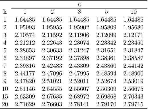
Table 1.1: Values ofb=b(P∗, k, c) as defined in (1.1.9)
c
k 1 2 3 5 10
1 1.64485 1.64485 1.64485 1.64485 1.64485 2 1.95993 1.95955 1.95902 1.95809 1.95680 3 2.10574 2.11592 2.11906 2.12099 2.12171 4 2.21212 2.22643 2.23074 2.23342 2.23450 5 2.28653 2.30633 2.31247 2.31651 2.31847 6 2.34897 2.37192 2.37898 2.38361 2.38587 7 2.39816 2.42483 2.43309 2.43860 2.44142 8 2.44177 2.47096 2.47995 2.48594 2.48900 9 2.47820 2.51021 2.52011 2.52674 2.53019 10 2.51146 2.54555 2.55607 2.56309 2.56675 15 2.63309 2.67635 2.68972 2.69868 2.70343 20 2.71629 2.76603 2.78141 2.79170 2.79715
In the Table 1.1, we provide the values of design constantb=b(P∗, k, c) given by equation
(1.1.9), for P∗ = 0.95, k = 1(1)10, 15, 20, and c = 1, 2, 3, 5, 10, for the covariance matrix Σ
defined in (1.1.8). As remarked earlier, for c= 1, the values of bhave been also tabulated in Tong (1969) and Gibbons, Olkin, and Sobel (1977). For the sake of completeness, we have included the
case c = 1, in the Table 1 as well, and, we must mention that the values provided in Table 1 for
c = 1 matches with the other two sources described above. The value of b is needed in order to implement the purely sequential procedure (1.3.1) and also to compute the optimal sample sizen∗
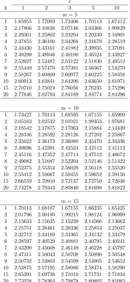
Table 1.2: Values of hν =hν(P∗, k, c) as defined in (1.2.4): P∗ =.95
c
k 1 2 3 5 10
m = 5
1 1.85955 1.77093 1.73406 1.70113 1.67412 2 2.17806 2.10838 2.07146 2.03366 1.99829 3 2.29301 2.25802 2.23294 2.20230 2.16901 4 2.37855 2.36100 2.34268 2.31679 2.28519 5 2.43430 2.43161 2.41982 2.39935 2.37091 6 2.48299 2.48946 2.48190 2.46524 2.43927 7 2.52027 2.53487 2.53122 2.51830 2.49512 8 2.55449 2.57470 2.57381 2.56367 2.54270 9 2.58267 2.60809 2.60977 2.60225 2.58358 10 2.60913 2.63841 2.64200 2.63650 2.61971 15 2.70710 2.75024 2.76056 2.76235 2.75296 20 2.77646 2.82783 2.84189 2.84774 2.84296
m = 10
1 1.73427 1.70113 1.68595 1.67155 1.65909 2 2.05163 2.02532 2.01021 1.99353 1.97681 3 2.18542 2.17875 2.17063 2.15884 2.14439 4 2.28346 2.28592 2.28126 2.27202 2.25867 5 2.35022 2.36173 2.36080 2.35470 2.34336 6 2.40696 2.42391 2.42524 2.42112 2.41112 7 2.45116 2.47352 2.47714 2.47512 2.46672 8 2.49082 2.51687 2.52204 2.52146 2.51422 9 2.52375 2.55354 2.56028 2.56118 2.55520 10 2.55412 2.58667 2.59455 2.59652 2.59150 15 2.66559 2.70910 2.72137 2.72750 2.72636 20 2.74278 2.79343 2.80840 2.81698 2.81822
m = 15
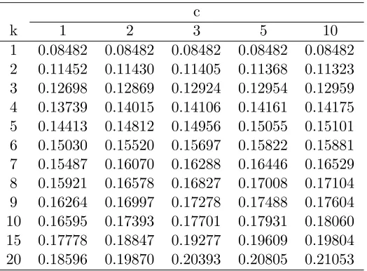
Table 1.3: Value ofg0(1) as defined in (1.3.11)
c
k 1 2 3 5 10
1 0.08482 0.08482 0.08482 0.08482 0.08482 2 0.11452 0.11430 0.11405 0.11368 0.11323 3 0.12698 0.12869 0.12924 0.12954 0.12959 4 0.13739 0.14015 0.14106 0.14161 0.14175 5 0.14413 0.14812 0.14956 0.15055 0.15101 6 0.15030 0.15520 0.15697 0.15822 0.15881 7 0.15487 0.16070 0.16288 0.16446 0.16529 8 0.15921 0.16578 0.16827 0.17008 0.17104 9 0.16264 0.16997 0.17278 0.17488 0.17604 10 0.16595 0.17393 0.17701 0.17931 0.18060 15 0.17778 0.18847 0.19277 0.19609 0.19804 20 0.18596 0.19870 0.20393 0.20805 0.21053
Next, in the Table 1.2, we provide the values of design constant hν =hν(P∗, k, c) which is
defined in (1.2.4), forP∗ = 0.95,k = 1(1)10, 15, 20,c= 1, 2, 3, 5, 10, andm= 5, 10, 15, for the
covariance matrix Σ defined in (1.8). The values of b for c= 1 have been also tabulated in Tong (1969) and Gibbons, Olkin, and Sobel (1977). Again, we have included the case c= 1 in the Table 1.2 and the values provided in Table 1.2 for c = 1 matches with the other two sources described above. The value ofhν is needed in order to implement the two-stage procedure (1.2.2).
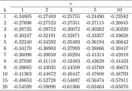
In the Tables 1.3 and 1.4, we provide the values of constants g0(1) and g00(1), respectively
fork = 1(1)10, 15, 20, and,c= 1, 2, 3, 5, 10. These constants, defined in (1.3.7), are needed to compute the asymptotic expansion provided in Theorem 1.3.1 (iii).
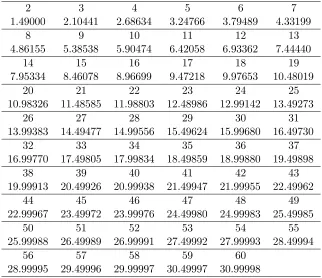
In the Table 1.5, we report the value of constant ν∗ =ν∗(k, c) as defined in (1.3.3). Note
that since the constant ν∗ depends on k and c only via k +c, we provide the values of ν∗ for
different values of k +c. Also, when k +c > 60, the second term on the right side of (1.3.3),
P∞
n=1n1E[(χ2n(k+c)−2n(k+c))+] is negligible (≤2·10−5). Therefore, in Table 5, we provide the
Table 1.4: Value ofg00(1) as defined in (1.3.11)
c
k 1 2 3 5 10
1 -0.34805 -0.27483 -0.25755 -0.24490 -0.23582 2 -0.27696 -0.27523 -0.27351 -0.27115 -0.26845 3 -0.28735 -0.29752 -0.30072 -0.30262 -0.30320 4 -0.30247 -0.32191 -0.32871 -0.33357 -0.33628 5 -0.32240 -0.34592 -0.35493 -0.36194 -0.36642 6 -0.34170 -0.36903 -0.37993 -0.38866 -0.39447 7 -0.36096 -0.39059 -0.40294 -0.41314 -0.42019 8 -0.37930 -0.41118 -0.42483 -0.43628 -0.44433 9 -0.39685 -0.43035 -0.44509 -0.45769 -0.46673 10 -0.41363 -0.44872 -0.46447 -0.47808 -0.48793 15 -0.48653 -0.52728 -0.54697 -0.56474 -0.57811 20 -0.54599 -0.59098 -0.61366 -0.63463 -0.65070
Next, in order to explain the role of second-order expansions to the reader, we look at
the expansions provided in Theorem 1.3.1, parts (ii) and (iii). From Theorem 1.3.1(ii), note that as a→ 0, E(N)−n∗
c = (ν∗ −2)(k +c)−1 +o(1). For example, for k = 10 the value of term
(ν∗ −2)(k +c)−1 can be computed using the Table 1.5 as, .40187 for c = 1, .41880 for c = 3,
and, .43072 for c= 5. Note that, these are the asymptotic values of the difference between E(N) and n∗
c for the selected values of k, c, and P∗. Later in this section, we use these to evaluate the
performance of the purely sequential procedure (1.3.1) for small or moderate sample sizes.
Now, we study the performance of the proposed procedures via Monte Carlo simulation
studies and also compare the procedures with the balanced ones, which correspond toc= 1.
The two-stage procedure (1.2.2) and the purely sequential procedure (1.3.1) were simulated
form= 10,c= 1,3,5,k = 10 andP∗ =.95, under a LFC. Without loss of generality we tookσ = 1
for the purpose of generating populations. We tookδ1 =−δ2, givinga=δ2(=δ, say). Next, using n∗
c = b 2σ2
a2 (c+1c ), we computed the values of δ corresponding to n∗c = 25,100,200,400 and 800.
Then, each procedure was independently repeated 1000 times. The performance of the two-stage
Table 1.5: Values of ν∗ as defined in (1.3.7)
2 3 4 5 6 7
1.49000 2.10441 2.68634 3.24766 3.79489 4.33199
8 9 10 11 12 13
4.86155 5.38538 5.90474 6.42058 6.93362 7.44440
14 15 16 17 18 19
7.95334 8.46078 8.96699 9.47218 9.97653 10.48019
20 21 22 23 24 25
10.98326 11.48585 11.98803 12.48986 12.99142 13.49273
26 27 28 29 30 31
13.99383 14.49477 14.99556 15.49624 15.99680 16.49730
32 33 34 35 36 37
16.99770 17.49805 17.99834 18.49859 18.99880 19.49898
38 39 40 41 42 43
19.99913 20.49926 20.99938 21.49947 21.99955 22.49962
44 45 46 47 48 49
22.99967 23.49972 23.99976 24.49980 24.99983 25.49985
50 51 52 53 54 55
25.99988 26.49989 26.99991 27.49992 27.99993 28.49994
56 57 58 59 60
28.99995 29.49996 29.99997 30.49997 30.99998
(The value on top is (k+c) and below it is ν∗)
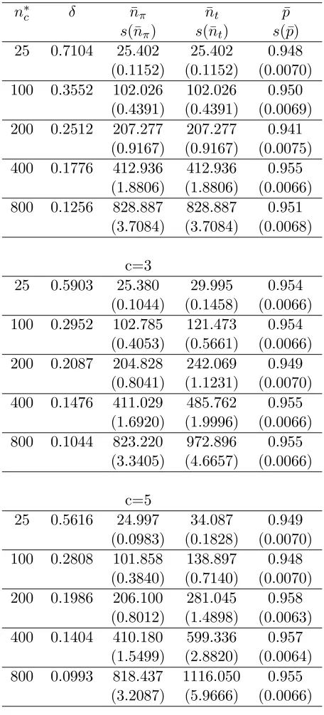
in the Table 1.7. In the Tables 1.6 and 1.7, we report the values of n∗
c, δ,n¯π: the average sample
size from π1,· · ·, πk, and ¯nt: the average sample size from π0, π1,· · ·, πk, and, ¯P: the proportion
of times all thek populations are partitioned correctly. We also report the standard errors of the reported estimates.
Note that as expected, using Theorems 1.2.1 and 1.3.1, the value of ¯P is close to or above the target value of 0.95, for all the cases considered and for both the procedures. One should
note that one of the inbuilt advantages of taking a larger sample from the control population
is to compensate for a smaller sample sizes from the other populations π1,· · ·, πk. This is clearly
evident for the casesc= 3 andc= 5 by comparing the values of ¯nπand ¯nt, in the Tables 1.6 and 1.7.
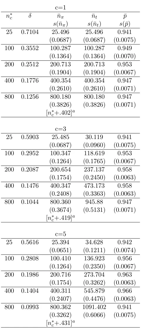
Table 1.6: Performance of the two-stage procedure (1.2.2)
c=1
n∗
c δ n¯π n¯t p¯
s(¯nπ) s(¯nt) s(¯p)
25 0.7104 25.402 25.402 0.948 (0.1152) (0.1152) (0.0070) 100 0.3552 102.026 102.026 0.950
(0.4391) (0.4391) (0.0069) 200 0.2512 207.277 207.277 0.941
(0.9167) (0.9167) (0.0075) 400 0.1776 412.936 412.936 0.955
(1.8806) (1.8806) (0.0066) 800 0.1256 828.887 828.887 0.951
(3.7084) (3.7084) (0.0068)
c=3
25 0.5903 25.380 29.995 0.954 (0.1044) (0.1458) (0.0066) 100 0.2952 102.785 121.473 0.954
(0.4053) (0.5661) (0.0066) 200 0.2087 204.828 242.069 0.949
(0.8041) (1.1231) (0.0070) 400 0.1476 411.029 485.762 0.955
(1.6920) (1.9996) (0.0066) 800 0.1044 823.220 972.896 0.955
(3.3405) (4.6657) (0.0066)
c=5
25 0.5616 24.997 34.087 0.949 (0.0983) (0.1828) (0.0070) 100 0.2808 101.858 138.897 0.948
(0.3840) (0.7140) (0.0070) 200 0.1986 206.100 281.045 0.958
(0.8012) (1.4898) (0.0063) 400 0.1404 410.180 599.336 0.957
(1.5499) (2.8820) (0.0064) 800 0.0993 818.437 1116.050 0.955
(3.2087) (5.9666) (0.0066)
Table 1.7: Performance of the purely sequential procedure (1.3.1)
c=1
n∗
c δ n¯π n¯t p¯
s(¯nπ) s(¯nt) s(¯p)
25 0.7104 25.496 25.496 0.941 (0.0687) (0.0687) (0.0075) 100 0.3552 100.287 100.287 0.949
(0.1364) (0.1364) (0.0070) 200 0.2512 200.713 200.713 0.953
(0.1904) (0.1904) (0.0067) 400 0.1776 400.354 400.354 0.947
(0.2610) (0.2610) (0.0071) 800 0.1256 800.180 800.180 0.947
(0.3826) (0.3826) (0.0071) [n∗
c+.402]a
c=3
25 0.5903 25.485 30.119 0.941 (0.0687) (0.0960) (0.0075) 100 0.2952 100.347 118.619 0.953
(0.1264) (0.1765) (0.0067) 200 0.2087 200.654 237.137 0.958
(0.1754) (0.2450) (0.0063) 400 0.1476 400.347 473.173 0.958
(0.2408) (0.3363) (0.0063) 800 0.1044 800.360 945.88 0.947
(0.3674) (0.5131) (0.0071) [n∗
c+.419]a
c=5
25 0.5616 25.394 34.628 0.942 (0.0651) (0.1211) (0.0074) 100 0.2808 100.410 136.923 0.956
(0.1264) (0.2350) (0.0067) 200 0.1986 200.716 273.704 0.963
(0.1754) (0.3262) (0.0063) 400 0.1404 400.311 545.879 0.966
(0.2407) (0.4476) (0.0063) 800 0.0993 800.362 1091.402 0.941
(0.3262) (0.6066) (0.0075) [n∗
c+.431]a
k= 10, P∗ =.95, andm= 10
optimal sample size. For example, for c = 1 and n∗
c = 800, the two stage procedure oversamples
by 29 or so observations. Such a behavior of the two-stage procedures is well documented in the
statistical literature. One way to eliminate over-sampling is to adopt a purely sequential procedure. Note that in the Table 1.7, the values ofn∗
c and ¯nπ are quite close and there does not appear to be
any oversampling. In the Table 1.7, we also provide the asymptotic value ofE(N)−n∗
c. Note that
even for small sample sizes, such as 25 or 100, the agreement between the asymptotic value and the
observed values is remarkable for all the three cases. In addition, using the Theorem 1.3.1(iii) and
the Tables provided in this section, one can easily verify that the observed ¯pvalue is in agreement with the asymptotic value. For example, in Table 1.7, for c = 5, we expect ¯p−P∗ to be close to
((k+c)n∗
c)−1{(ν∗−2)g0(1) +g00(1) (=.0004536) and the observed difference is .006 with standard
error of .0067.
Remark 1.4.1: It is important to note that within the Table 1.6 , and, also within the Table 1.7,
one cannot compare the blocks corresponding to different values of c with one another. This is so because even though the n∗
c values are same in the three blocks, the value of δ is smaller for the
largercvalue. Also, note that in Tables 6 and 7, forc= 3 andc= 5, the value of ¯nt is significantly
larger than that of ¯nπ, as we take more observations from π0. In other words, since n∗c denotes
the optimal sample size from π1,· · ·, πk, it needs to be compared with ¯nπ. An alternative way to
compute ¯nt would be to divide the number of samples collected fromπ0 bycbefore computing the
Chapter 2
Assessing Robustness of Procedures
2.1
Introduction
In real world applications, the partition problem is a routine problem which gets applied in
numerous different areas, such as, biological sciences, medical sciences, agricultural sciences, etc, to
name a few, in order to compare newer treatments with a control. However, a large proportion of
the statistical theory is developed for the normal distribution case and also under various assump-tions.
In this chapter, we consider the robustness of various partition procedures known in the
statistical literature, including the ones proposed in Chapter 1, from the point of view of mild to
moderate departures from the assumptions. The goal of the study is to document the performance
of the different procedures under such several mild/moderate departures.
2.2
Description of The Procedures
In this chapter, we have selected a few procedures to study the robustness issues. It should
be noted that the literatures is quite rich and has many such procedures and inclusion of all such
procedures in not practical. However, we have selected a few, to illustrate our point. The selected
procedures are somewhat the standard procedures and have been cited regularly in the statistical
literature.
The procedure described below was developed by Tong (1969).
Letm >1 be a pre-assigned positive integer indicating the starting sample size. We collect
m observations from each of thek+ 1 populations, and compute the estimator ofσ2 given by
S2=ν−1 k
X
i=0 m
X
j=1
[Xi j−m−1( m
X
n=1 Xi j)]2
whereν= (k+ 1)(m−1). After this, in the second stage we collectN−madditional samples from each population, where N is the smallest integer satisfying
N ≥max{m, <2h2νSν2/a2 >}. (2.2.1)
Then we partition the k populations based on N samples using (1.1.5). Note that hν is available
in the Table 2 in Tong (1969).
Three Stage Procedure (TS): In a three-stage procedure, the samples are collected in three
batches. The procedure stated below and its fine tuned version were developed by Datta and Mukhopadhyay(1998).
Choose and fix ρ ∈ (0, 1), collect m observations from each population as the starting sample size, and compute
T =max{m, <2ρb2Sm2a−2 >+1}.
CollectT −m additional samples from each populations in the second batch and compute:
N =max{T, <2b2ST2a−2 >+1}.
In the third batch, we collect N −T additional samples from each population, compute overall sample means and apply the same decision as described in (1.1.5), where < x >=largest integer
Fined Tuned Three Stage Procedure (TSR):
Choose and fix ρ ∈ (0, 1), collect m observations from each population as the starting sample size, and compute
T =max{m, <2ρb2Sm2a−2 >+1}.
CollectT −m additional samples from each populations in the second batch and compute:
N =max{T, <2b2ST2a−2+ >+1}.
In the third batch, we collect N −T additional samples from each population, compute overall sample means and apply the same decision as described in (1.1.5), where < x >=largest integer
< x, b is available in table 1 in Tong (1969), and =ρ−1(k+ 1)−1[2− {g00(1)/g0(1)}]−1/2. Here g(·) is a special case for c= 1 of the g(·), which is defined in the Chapter 1.
Purely Sequential Procedure (PS): This procedure and its fine tuned version were developed
by Datta and Mukhopadhyay (1998).
Define N = inf{n ≥ m : n ≥ 2b2Sn2/a2}. Then apply the decision rule as described in (1.1.5) based on N samples, where bis available in the Table 1 in Tong (1969).
Fined Tuned Purely Sequential Procedure (PSR):
Define N =inf{n≥m: n+≥2b2S2
n/a2}. Then apply the decision rule as described in
(1.1.5) based onN samples, wherebis available in the Table 1 in Tong (1969). Where, the constant
= (k+ 1)−1[(ν−2) +g00(1)/g0(1)] and g(·) is same as the one introduced for the fine tuned three
stage procedure.
Purely Sequential Procedure with Elimination (ES): This procedure can eliminate and
Solanky (2001). This procedure has the following steps.
(1) Start with the sample size m(>1) samples from each population, compute:
Xi m = m
X
j−1
Xi j/m, Si m2 = m
X
j=1
(Xi j−Xi m)2/(m−1),
S2=
k
X
i=0
Si m2 /k, aλ=ηf S2/a, Wλ = [aλ/λ].
(2) Draw one observation from those populations, which have not been eliminated, until
(i)m≥Wλ, or
(ii) all the populations have been partitioned, and then do step (4).
(3) Within each population that to be partitioned, partition any populations into SB for which
r
X
j=1
Xi j < r
X
j=1
(X0 j+d−aλ+rλ),
partition any populations into SG for which
r
X
j=1
Xi j > r
X
j=1
(X0 j+d+aλ−rλ).
(4) ifm=Wλ, then get one more observation from the populations haven’t been partitioned, and
them apply decision rule (1.1.5) to those populations. Here η could be found in table 1 in Solanky (2001) and λ=a/(2j).
Unbalanced Procedures
There are two kinds of unbalanced procedures, which are the two-stage unbalanced
proce-dure(UDS) and purely sequential unbalanced procedure(UPS). The details of these procedures
2.3
Performance of the Procedures
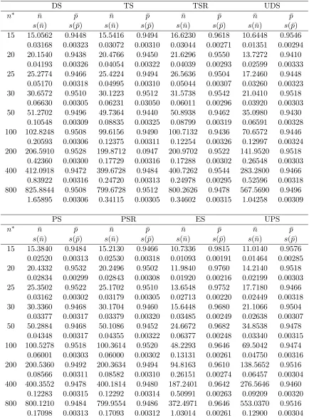
We start by simulating all the selected procedures when all of the assumptions are
satis-fied. We generated k + 1 groups of samples, which are independent within each group and from independent and normally distributed populations. We choose k = 10, and the populations are assumed under the LFC and the variance of the populations was taken to be 1, without the loss of generality. We took µ0 = 0 and δ1 =−δ2, giving a=δ2(=δ, say). Next, using n∗ = 2b
2σ2 a2 , we
computed the values of δ corresponding to n∗ = 15, 20, 25, 30, 50, 100, 200, 400 and 800. The
values are in the following table:
Table 2.1: Values ofδ for specified optional sample sizes
n∗ 15 20 25 30 50 100 200 400 800
δ=−δ1=δ2 0.9171 0.7942 0.7103 0.6485 0.5023 0.3552 0.2511 0.1776 0.1256
We took the starting sample size to bem= 10,P∗=.95,ρ= 1
4, for TS and TSR andj= 2
for the ES. For each value of δ, each procedure was independently repeated for 5000 times and we recorded the sample size as well as whether the partition is a CD or not, in each iteration. The
aver-age sample sizes and the actual percentaver-ages of CD for the procedures are displayed in the Table 2.2.
To summarize, all the procedures are working quite well with the estimated probability of
CD (= ¯p) being close to its target value and the average sample size (= ¯n) being close to its optimal valuen∗.
2.4
Departure from Normality
2.4.1 Symmetric Distributions Case
In this section, we restrict our attention to symmetric distributions only. For the underlying
distributions, we chose a variety of non-normal distributions to represent a wide range of symmetric
Table 2.2: Simulation Results under Normal Distribution Assumption
DS TS TSR UDS
n∗ n¯ p¯ ¯n p¯ n¯ p¯ n¯ p¯
s(¯n) s(¯p) s(¯n) s(¯p) s(¯n) s(¯p) s(¯n) s(¯p) 15 15.0562 0.9448 15.5416 0.9494 16.6230 0.9618 10.6448 0.9546
0.03168 0.00323 0.03072 0.00310 0.03044 0.00271 0.01351 0.00294 20 20.1540 0.9438 20.4766 0.9450 21.6296 0.9550 13.7272 0.9410
0.04193 0.00326 0.04054 0.00322 0.04039 0.00293 0.02599 0.00333 25 25.2774 0.9466 25.4224 0.9494 26.5636 0.9504 17.2460 0.9448
0.05170 0.00318 0.04995 0.00310 0.05044 0.00307 0.03260 0.00323 30 30.6572 0.9510 30.1223 0.9512 31.5738 0.9542 21.0410 0.9518
0.06630 0.00305 0.06231 0.03050 0.06011 0.00296 0.03920 0.00303 50 51.2702 0.9496 49.7364 0.9440 50.8938 0.9462 35.0980 0.9430
0.10548 0.00309 0.08835 0.00325 0.08799 0.00319 0.06591 0.00328 100 102.8248 0.9508 99.6156 0.9490 100.7132 0.9436 70.6572 0.9446
0.20593 0.00306 0.12375 0.00311 0.12254 0.00326 0.12997 0.00324 200 206.5910 0.9528 199.8712 0.0947 200.9702 0.9522 141.9520 0.9518
0.42360 0.00300 0.17729 0.00316 0.17288 0.00302 0.26548 0.00303 400 412.0918 0.9472 399.6728 0.9484 400.7262 0.9544 283.2800 0.9466
0.83922 0.00316 0.24720 0.00313 0.24978 0.00295 0.52596 0.00318 800 825.8844 0.9508 799.6728 0.9512 800.2626 0.9478 567.5690 0.9496
1.65895 0.00306 0.34115 0.00305 0.34602 0.00315 1.04258 0.00309
PS PSR ES UPS
n∗ n¯ p¯ ¯n p¯ n¯ p¯ n¯ p¯
s(¯n) s(¯p) s(¯n) s(¯p) s(¯n) s(¯p) s(¯n) s(¯p) 15 15.3840 0.9484 15.2130 0.9466 10.7336 0.9815 11.0140 0.9576
0.02520 0.00313 0.02530 0.00318 0.01093 0.00191 0.01464 0.00285 20 20.4332 0.9532 20.2496 0.9502 11.9840 0.9760 14.2140 0.9518
0.02834 0.00299 0.02843 0.00308 0.01920 0.00216 0.02199 0.00303 25 25.3502 0.9522 25.1702 0.9510 13.6548 0.9752 17.7180 0.9466
0.03162 0.00302 0.03179 0.00305 0.02713 0.00220 0.02449 0.00318 30 30.3360 0.9468 30.1704 0.9460 15.6448 0.9680 21.1066 0.9504
0.03377 0.00317 0.03379 0.00320 0.03485 0.00249 0.02638 0.00307 50 50.2884 0.9468 50.1086 0.9452 24.6672 0.9682 34.8538 0.9478
0.04348 0.00317 0.04355 0.00322 0.06377 0.00248 0.03340 0.00315 100 100.5278 0.9518 100.3614 0.9520 48.2293 0.9646 69.5042 0.9474
0.06001 0.00303 0.06000 0.00302 0.13131 0.00261 0.04750 0.00316 200 200.5360 0.9492 200.3634 0.9494 94.8163 0.9610 138.5652 0.9516
0.08566 0.00311 0.08582 0.00310 0.26151 0.00274 0.06457 0.00304 400 400.3552 0.9478 400.1814 0.9480 187.2401 0.9642 276.5646 0.9460
0.12283 0.00315 0.12292 0.00314 0.50991 0.00263 0.09209 0.00320 800 800.1210 0.9484 799.9554 0.9486 372.4971 0.9646 553.0370 0.9516
We included two Student t distributions with 10 and 20d.f. respectively, a Laplace distri-bution and three mixture of normal distridistri-butions with 2, 4 and 6 squared Mahalanobis distances, respectively, to represent a family of distributions with varying kurtosis. Thecdf of these mixture-normal distributions was
Fi(x) =πi1N(x;µi1, σ2) +πi2N(x;µi2, σ2), (2.4.1)
whereN(x;µi1, σ2) andN(x;µi2, σ2) are Gaussian random variables with locations (µi1, µi2) and a
common covariance,σ2 andπ
i1+πi2 = 1 are the mixing proportions. To specify a mixture-normal
distribution with a given mean and variance 1, we define
∆ = (µi1−µi2)2σ−2 (2.4.2)
as squared Mahalanobis distance associated with the distribution. We choose the mean and
vari-ance of the component normal distributions, such that the mixture-normal distribution will have
squared Mahalanobis distances as 2, 4 and 6 respectively. The parameters for such distribution
with mean µ= 0 are in the Table 2.3:
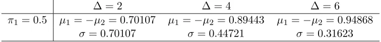
Table 2.3: The Parameters for Symmetrical Mixture-Normal Distributions
∆ = 2 ∆ = 4 ∆ = 6
π1 = 0.5 µ1=−µ2 = 0.70107 µ1 =−µ2 = 0.89443 µ1 =−µ2= 0.94868 σ= 0.70107 σ= 0.44721 σ = 0.31623
As before, we choose k = 10, and assumed the k control populations have some non-normal distributions in the same location family and the control population still has the standard
normal distribution. Also, we assumed that the populations are independent and they are under
LFC and have common variance σ2 = 1, without the loss of generality. Note that the mixture-normal distributions with the parameters given in Table 2.3 have variance σ2 = 1. Hence, the
for the student t and Laplace distributions, we chose the ones with variance σ2 = 1 from their location-scale family to be the location families, which include the distributions of the non-control
populations. The value of δ1 and δ2 were set in the same way as in the first paragraph in Section
2.3 to specify the distributions of the non-control populations from the location families described
above. Then we generated k+ 1 groups of samples from such populations, each group is corre-sponding to one population, for our robustness study.
We took the starting sample size to be m = 10, P∗ = .95, ρ = 1
4, for TS and TSR and j = 2 for the ES. For each distribution we mentioned above and each value of δ, each procedure was repeated 5000 times independently, and the value of ¯nand s(¯n), ¯p and s(¯p) are recorded and displayed in Tables 2.4 - 2.9.
From the Tables 2.7, 2.8 and 2.9, we see that for the distributions with lighter tails than
normal distributions, i.e., with smaller kurtosis, the procedures perform well. The values of ¯p are increasing as the tails of the distributions become lighter.
The Table 2.4, 2.5 and 2.6, indicate that the performance of the procedures with heavy
tails. Generally, the heavier the tail, the smaller the ¯p for all the procedures and in all the cases. We also found that the ES is robust to the heavy-tailedness. Since the ES procedure is based on
some inequalities and the ¯p values are generally overshooting the target, the ES procedure works well even under such moderate violation. The validity of the UPS procedure is marginally affected
by tailedness. The performance of the other six procedures is moderately affected by
heavy-tailedness.
From the Tables, it is difficult to pin point the exact robustness of the procedures. However,
it is important to note that the worst performance is for TSR withn∗ = 50, giving ¯p= 0.9364. Note
that this worst case is well within 2 standard errors of the target value. Hence, our conclusion is that
Table 2.4: Simulation Results fort20 Distribution
DS TS TSR UDS
n∗ n¯ p¯ ¯n p¯ n¯ p¯ n¯ p¯
s(¯n) s(¯p) s(¯n) s(¯p) s(¯n) s(¯p) s(¯n) s(¯p) 15 15.0024 0.9418 15.4900 0.9498 16.6312 0.9644 10.6444 0.9514
0.03329 0.00331 0.03213 0.00309 0.03321 0.00262 0.01379 0.00304 20 20.1856 0.9462 20.5038 0.9484 21.6098 0.9606 13.7262 0.9438
0.04440 0.00319 0.04287 0.00313 0.04253 0.00275 0.02751 0.00326 25 25.2694 0.9490 25.4130 0.9500 26.6638 0.9538 17.2460 0.9458
0.05635 0.00311 0.05449 0.00308 0.05371 0.00297 0.03523 0.00320 30 30.6144 0.9474 30.5438 0.9476 31.6022 0.9508 20.9094 0.9426
0.06818 0.00316 0.06449 0.00315 0.06340 0.00306 0.04238 0.00329 50 51.0944 0.9436 49.5350 0.9406 50.7556 0.9510 35.0158 0.9436
0.11229 0.00326 0.09412 0.00334 0.09291 0.00305 0.06971 0.00326 100 102.6926 0.9482 99.5318 0.9472 100.6496 0.9480 70.5460 0.9512
0.21929 0.00313 0.13294 0.00316 0.13474 0.00314 0.13708 0.00305 200 205.8878 0.9478 199.6950 0.9482 200.9040 0.9518 141.5770 0.9446
0.45609 0.00315 0.19233 0.00313 0.18828 0.00303 0.28342 0.00324 400 413.2788 0.9488 399.4182 0.9514 401.1600 0.9562 284.2158 0.9510
0.90211 0.00312 0.26372 0.00304 0.26234 0.00289 0.55626 0.00305 800 827.1610 0.9420 799.3644 0.9452 800.9254 0.9510 568.7584 0.9486
1.82051 0.00331 0.36993 0.00322 0.37371 0.00305 1.12719 0.00312
PS PSR ES UPS
n∗ n¯ p¯ ¯n p¯ n¯ p¯ n¯ p¯
s(¯n) s(¯p) s(¯n) s(¯p) s(¯n) s(¯p) s(¯n) s(¯p) 15 15.4140 0.9470 15.2336 0.9460 10.7394 0.9796 11.0422 0.9616
0.02669 0.00317 0.02673 0.00320 0.01112 0.00200 0.01547 0.00272 20 20.3616 0.9498 20.1926 0.9484 11.9849 0.9778 14.2002 0.9528
0.03043 0.00309 0.03069 0.00313 0.01961 0.00208 0.02315 0.00300 25 25.3738 0.9504 25.1986 0.9506 13.6879 0.9716 17.6798 0.9488
0.03355 0.00307 0.03361 0.00306 0.02808 0.00235 0.02569 0.00312 30 30.3482 0.9540 30.1722 0.9540 15.5872 0.9710 21.0728 0.9538
0.03702 0.00296 0.03723 0.00296 0.03566 0.00237 0.02827 0.00297 50 50.4142 0.9482 50.2378 0.9480 24.6208 0.9656 34.9134 0.9490
0.04710 0.00313 0.04706 0.00314 0.06701 0.00258 0.03558 0.00311 100 100.3500 0.9524 100.1764 0.9518 47.9847 0.9664 69.4396 0.9492
0.06624 0.00301 0.06623 0.00303 0.13321 0.00255 0.04993 0.00311 200 200.3658 0.9502 200.1868 0.9506 94.8547 0.9662 138.5380 0.9524
0.09233 0.00308 0.09232 0.00306 0.27186 0.00256 0.07047 0.00301 400 400.2880 0.9480 400.1088 0.9480 186.3133 0.9564 276.5396 0.9478
0.13098 0.00314 0.13102 0.00314 0.54313 0.00289 0.09826 0.00315 800 800.4784 0.9470 800.2932 0.9468 371.3969 0.9562 552.8602 0.9514
Table 2.5: Simulation Results fort10 Distribution
DS TS TSR UDS
n∗ n¯ p¯ ¯n p¯ n¯ p¯ n¯ p¯
s(¯n) s(¯p) s(¯n) s(¯p) s(¯n) s(¯p) s(¯n) s(¯p) 15 15.0414 0.9462 15.5194 0.9504 16.6158 0.9580 10.7104 0.9534
0.03716 0.00319 0.03608 0.00307 0.03640 0.00284 0.01570 0.00298 20 20.1950 0.9458 20.5152 0.9510 21.6144 0.9486 13.7524 0.9438
0.04849 0.00320 0.04678 0.00305 0.04793 0.00312 0.02956 0.00326 25 25.4304 0.9472 25.5588 0.9474 26.7004 0.9598 17.3444 0.9442
0.06260 0.00316 0.06031 0.00316 0.05915 0.00278 0.03850 0.00325 30 30.6018 0.9508 30.5184 0.9498 31.4970 0.9532 20.8838 0.9442
0.07407 0.00306 0.06986 0.00309 0.06932 0.00299 0.04561 0.00325 50 51.2114 0.9462 49.5132 0.9406 50.6020 0.9506 35.1008 0.9460
0.12259 0.00319 0.10240 0.00334 0.10268 0.00306 0.07537 0.00320 100 102.9150 0.9504 99.3822 0.9442 100.1190 0.9420 70.6942 0.9452
0.24633 0.00307 0.15121 0.00325 0.14953 0.00331 0.15011 0.00322 200 205.6234 0.9444 199.1190 0.9438 200.3764 0.9530 141.3906 0.9508
0.48899 0.00324 0.20941 0.00326 0.20819 0.00299 0.30073 0.00306 400 413.5736 0.9434 399.3724 0.9438 400.7564 0.9476 284.7942 0.9500
1.03575 0.00327 0.29783 0.00326 0.29242 0.00315 0.62894 0.00308 800 826.0084 0.9436 799.5828 0.9506 801.4692 0.9486 567.8116 0.9428
1.97272 0.00326 0.41629 0.00306 0.42254 0.00312 1.21229 0.00328
PS PSR ES UPS
n∗ n¯ p¯ ¯n p¯ n¯ p¯ n¯ p¯
s(¯n) s(¯p) s(¯n) s(¯p) s(¯n) s(¯p) s(¯n) s(¯p) 15 15.3318 0.9510 15.1532 0.9478 10.7509 0.9800 11.0424 0.9524
0.02920 0.00305 0.02928 0.00315 0.01161 0.00198 0.01642 0.00301 20 20.2626 0.9460 20.0852 0.9446 11.9635 0.9742 14.2442 0.9496
0.03350 0.00320 0.03383 0.00324 0.02041 0.00224 0.02496 0.00309 25 25.3076 0.9516 25.1230 0.9506 13.6690 0.9730 17.6604 0.9544
0.03655 0.00304 0.03670 0.00306 0.03015 0.00229 0.02872 0.00295 30 30.3390 0.9544 30.1632 0.9520 15.7363 0.9644 21.0422 0.9506
0.03983 0.00295 0.03998 0.00302 0.03917 0.00262 0.03015 0.00306 50 50.3626 0.9510 50.1842 0.9510 24.7543 0.9650 34.8968 0.9520
0.05196 0.00305 0.05209 0.00305 0.07137 0.00260 0.03868 0.00302 100 100.3638 0.9576 100.1866 0.9570 47.9579 0.9614 69.3964 0.9464
0.07302 0.00285 0.07305 0.00287 0.14168 0.00272 0.05480 0.00319 200 200.3668 0.9474 200.1964 0.9480 94.3464 0.9620 138.5110 0.9548
0.10386 0.00316 0.10396 0.00314 0.28114 0.00270 0.07716 0.00294 400 400.4982 0.9490 400.3254 0.9490 186.7014 0.9578 276.6496 0.9522
0.14545 0.00311 0.14537 0.00311 0.57102 0.00284 0.10927 0.00302 800 800.7582 0.9530 800.5872 0.9528 371.7556 0.9642 552.7822 0.9494
Table 2.6: Simulation Results for Laplace Distribution
DS TS TSR UDS
n∗ n¯ p¯ ¯n p¯ n¯ p¯ n¯ p¯
s(¯n) s(¯p) s(¯n) s(¯p) s(¯n) s(¯p) s(¯n) s(¯p) 15 15.0680 0.9370 15.5354 0.9444 16.6516 0.9598 10.8632 0.9508
0.04599 0.00344 0.04480 0.00324 0.04536 0.00278 0.01920 0.00306 20 20.1848 0.9428 20.4912 0.9470 21.6520 0.9526 13.7868 0.9396
0.06267 0.00328 0.06050 0.00317 0.05928 0.00301 0.03629 0.00337 25 25.3860 0.9420 25.5094 0.9444 26.5384 0.9546 17.2860 0.9384
0.07714 0.00331 0.07373 0.00324 0.07490 0.00294 0.04595 0.00340 30 30.4968 0.9418 30.3122 0.9410 31.4456 0.9504 20.8304 0.9394
0.09307 0.00331 0.08494 0.00333 0.08593 0.00307 0.05563 0.00337 50 51.3894 0.9412 49.2110 0.9370 50.3252 0.9432 35.1426 0.9430
0.15312 0.00333 0.12471 0.00344 0.12572 0.00327 0.09162 0.00328 100 103.1948 0.9436 98.7002 0.9396 99.7328 0.9452 70.8246 0.9450
0.30878 0.00326 0.18795 0.00337 0.18853 0.00322 0.18572 0.00322 200 205.7662 0.9466 198.2938 0.9498 200.1640 0.9450 141.3786 0.9410
0.62266 0.00318 0.26657 0.00309 0.26400 0.00322 0.37134 0.00333 400 411.7306 0.9430 398.4490 0.9524 399.0816 0.9550 283.0924 0.9484
1.24781 0.00328 0.37917 0.00301 0.38075 0.00293 0.74708 0.00313 800 826.4782 0.9414 798.7574 0.9470 799.8952 0.9490 568.7938 0.9466
2.46818 0.00332 0.54711 0.00317 0.53572 0.00311 1.46721 0.00318
PS PSR ES UPS
n∗ n¯ p¯ ¯n p¯ n¯ p¯ n¯ p¯
s(¯n) s(¯p) s(¯n) s(¯p) s(¯n) s(¯p) s(¯n) s(¯p) 15 15.2296 0.9458 15.0444 0.9428 10.7962 0.9766 11.1348 0.9548
0.03596 0.00320 0.03594 0.00328 0.01282 0.00214 0.01885 0.00294 20 20.2624 0.9452 20.0806 0.9434 12.0138 0.9710 14.0720 0.9498
0.04245 0.00322 0.04256 0.00327 0.02293 0.00237 0.03051 0.00309 25 25.2372 0.9434 25.0656 0.9420 13.7042 0.9682 17.5930 0.9418
0.04812 0.00327 0.04839 0.00331 0.03385 0.00248 0.03421 0.00331 30 30.2208 0.9480 30.0352 0.9462 15.6556 0.9658 20.9754 0.9518
0.05086 0.00314 0.05091 0.00319 0.04326 0.00257 0.03779 0.00303 50 50.2000 0.9486 50.0232 0.9484 24.6831 0.9648 34.8032 0.9472
0.06578 0.00312 0.06584 0.00313 0.08269 0.00261 0.04778 0.00316 100 100.2728 0.9488 100.0888 0.9480 48.0851 0.9586 69.4130 0.9524
0.09313 0.00312 0.09322 0.00314 0.16771 0.00282 0.06793 0.00301 200 200.1482 0.9540 199.9750 0.9546 94.3808 0.9558 138.4542 0.9456
0.13059 0.00296 0.13069 0.00294 0.33727 0.00291 0.09708 0.00321 400 400.0282 0.9454 399.8514 0.9454 186.3922 0.9550 276.5936 0.9518
0.18563 0.00321 0.18575 0.00321 0.65378 0.00293 0.13509 0.00303 800 800.0730 0.9552 799.9012 0.9560 369.6602 0.9554 552.6472 0.9490