Genetic analysis of longevity data in the UK: present practice and considerations for the future
7
0
0
Full text
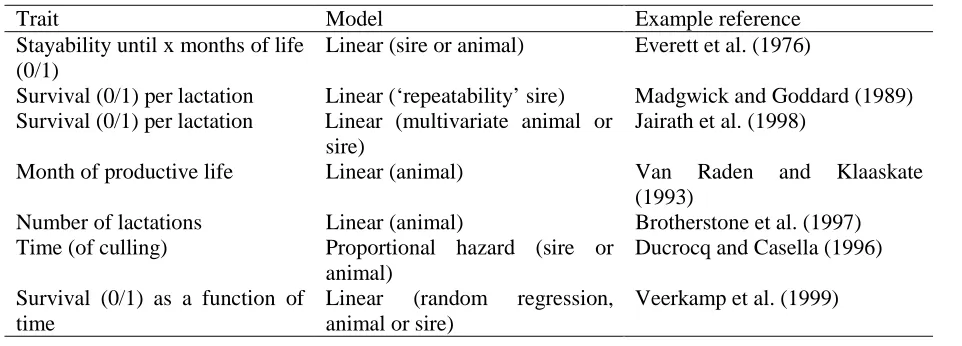
(2) Table 1 shows a wide varieties in traits and models. Most linear models do not model the trait of interest as a function of time (except Veerkamp et al. 1999).. n + pn + pn* pn+1 + pn* pn+1* pn+2 + ….. For the current UK evaluation, the survival probabilities p for lactation 1 to 5 are 0.73, 0.67, 0.71, and 0.71, respectively. It was assumed that p remains constant after lactation 5, i.e. 0.71. Using these conditional probabilities, a predefined set of lifespans can been set up. For example, if an animal had only time to finish 2 lactation and was censored at t=2 (i.e., had no time for lactation 3), then the assigned lifespan (LS) is:. The purpose of this study is to describe the current method of evaluation for longevity in the UK, to discuss other possible approaches to analyse discrete longevity data, to discuss remaining problems with the analysis of longevity, and to suggest future developments. 2. Lifespan concept and evaluations. LS. =. 2.1 Data quality = =. A natural by-product of an efficient milk recording programme is that we can describe the life-history of a dairy cow from entering the milking herd to culling. Specific time points in the life history are dates at which a cow calved, was dried off, and started a subsequent lactation. Unfortunately, in the UK until recently (end of 1992) the only information available to researchers was the number of qualified lactations of a cow in milk recording, where a qualified lactation means a lactation length of at least 200 days. In addition, there are no reliable records kept after lactation 5. These data quality problems mean that (i) there is no record of culling before day 200 in the first lactation, (ii) the resolution of longevity measures is one lactation, and (iii) the records of all cows which have produced five lactations are censored, i.e. we do not know whether these cows were culled after lactation 5 or went on to produce further lactations.. 2 + p2 + p2*p3 + p2*p3*p4 + p2*p3*p4*p5 + ….. 2 + 0.67 + 0.67*0.71 + ... 4.3. Hence, prediction of expected lifespan is based upon population-wide average conditional survival probabilities. Note that there can be cows with censored records which have larger (predicted) values for lifespan than the largest value for an uncensored observation (i.e., LS=4). This is based upon the fact that we know that on average cows which have survived until lactation 3 and are still in the herd will have a lifespan greater than 4 lactations. If all pi values are constant (p), and cows have had no time restriction in the opportunity to express LS, then, Prob(LS=x) = (1-p)px-1 [x=1,2,3, ....] i.e. LS has a geometric distribution (Brotherstone et al., 1997), with mean and variance. 2.2 Concept of lifespan E(LS) = var(LS)=. Brotherstone et al. (1997) developed a simple method to deal with the UK longevity data, and which could use existing animal model BLUP software. They introduced the concept of lifespan, which is the number of lactations a cow has survived, or is expected to survive. If pn is the probability of survival to lactation n+1 of an animal that has survived to complete lactation n, the expected lifespan of a random animal that has completed n lactations but has not had time to complete n + 1 lactations is (Brotherstone et al., 1997):. 1/(1-p) = p/(1-p)2. 1 + p/(1-p). The probability that LS is equal or larger than value T is, Prob(LS>=T). = 1 – Prob(LS<T) = 1 – (1 – pT-1) = pT-1. This corresponds to the definition of ‘stayability until lactation T’ which has been used in the literature (see Table 1).. 17.
(3) The concept of lifespan is similar to the method of longevity analysis in the USA (Van Raden and Klaaskate, 1993), where the length of productive life (months in milk) is used as the trait of interest, and future records are predicted using phenotypic multiple regression. The main differences are that in the UK evaluation a phenotypic regression on milk yield in the first lactation is used in the genetic evaluation, and that the parameterisation is in terms of number of lactations instead of number of months of productive life. Both methods use population-wide phenotypic regression to predict future records.. as the daughters of a bull get older, from most emphasis on type traits to most emphasis on lifespan scores. Bowman et al. (1996) used customised selection indices to predict overall profit, including EBV on survival and type traits in (multivariate) index calculations, which results in the same re-weighting of information. The Canadian system of EBV for herd life also combined survival and type data (Jairath et al., 1998). 3. Analysis of discrete data Methods which model the risk of culling (or ‘hazard’) are theoretically better, since they take account of the appropriate distribution of the data and allow better fixed effects structures (see Ducrocq, 1999, and references therein). The Weibull model has been used widely (due to the availability of appropriate software) to model the baseline hazard rate in dairy cattle. Our discrete data, i.e., failure times of 1,2, 3, 4, or 5, are discrete, and violate the assumption of a continuous time variate. However, the conditional probabilities of survival in each lactation are fairly constant over time (Brotherstone et al., 1997), as one would expect from an exponential distribution of the hazard rate. Therefore, we used a Weibull model to analyse lifespan, and compared heritability estimates and correlations between EBV of sires using either the Weibull model or lifespan (Lubbers et al., 1999). Lifespan (LS) records of 21497 cows, daughters of 487 sires, were analysed using a sire model in both approaches. In addition to LS, the logarithm of lifespan was analysed using the same linear model as used for the analysis of LS. Heritabilities for LS and log(LS) were about 0.05, and 0.07 from the Weibull model on a log-scale. A transformation of that heritability to the observed scale gave a value of 0.17. Correlations between EBV for sires calculated from linear and proportional hazard models were high, with absolute value between 0.93 and 0.98. For example, the correlation between EBV for LS from the linear model and EBV from the Weibull model in which no timedependent effects were fitted was –0.97. It was concluded that it may be appropriate to use discrete lactation data in a Weibull model. In subsequent study, we compared a Weibull model and a grouped-data discrete proportional hazard model using a larger data. 2.3 Genetic evaluation for herd life The genetic evaluation for herdlife in the UK was described by Brotherstone et al. (1998). In addition to the direct information used from the lifespan scores of individual cows (as described in the previous section), information from type traits are used to predict herdlife. These sources of information are combined into a bivariate analysis of lifespan score and a phenotypic index of three type traits (foot angle, udder depth and teat length). The index weights for the type traits were those previously used in a national index to predict herd life from type data only. The index of type traits was created to scale the problem down from a 4-variate to a bivariate problem, without much loss of information (Brotherstone et al., 1998). Assumed heritabilities for these two traits were 0.06 and 0.44, respectively (Brotherstone et al., 1998), estimated from a data set in which all cows had the opportunity to complete 5 lactations. The bivariate animal model contained the fixed effects of herd-year of first calving, month of first calving, age at first calving (covariate) and the deviation of first lactation milk yield from the herd mean (covariate) for the lifespan scores, and herd-classification visit, month of first calving, age at first calving (covariate) and stage of lactation of inspection (covariate) for the type index (Brotherstone et al., 1998). Bull proofs for herd life (lifespan) were first published in August 1998 by the Animal Data Centre (ADC). The range of predicted transmitting abilities is approximately 1 lactation. The advantage of using a bivariate analysis is that most of the relevant information is used to predict herdlife, and that there is a logical re-weighting of information. 18.
(4) set 85367 records (Yazdi et al, 1999). In the discrete model the discrete hazard for each interval was modelled (Ducrocq, 1999, and these proceedings). Correlations between EBV for the 284 sires were very high, >0.98 for the different models investigated. It was concluded that ignoring the discrete and grouped data structure in the Weibull model did not have a significant impact on sire ranking.. herdlife in months is the trait of interest, the effect of the end-of-quota year or BSE cohort culling could be fitted, in particular in proportional hazards models with timedependent covariates (e.g., Ducrocq 1999, and references therein). A particular benefit from a better data-stream even with a 0/1 analysis is that information is known sooner. At present, we have to wait over a year before deciding a cow has left the herd. Multivariate analysis of binary survival traits. There appears to be some confusion in the literature about the covariance structure of binary survival traits in genetic evaluations using a sire or animal model. For example, Boettcher et al. (1999) tried to estimate variance components for survival in the first three lactations using an animal model (estimating 6 genetic and 6 environmental covariance components), but encountered problems with convergence. The likely cause, which was pointed out by Madgwick and Goddard (1989) and Visscher and Goddard (1995) is that there is no environmental covariance across lactations. Consider survival in two lactations, and let 1 denote survival. Then, records are either {1 0}, {1 1}, or {0 undefined/missing}. The phenotypic covariance is zero, because all cows with an observation in lactation 2 have the same score (1) in the first lactation. Essentially the definition of survival in lactation 2 is conditional on survival in lactation 1. When using either a sire or animal model it seems incorrect to estimate a covariance component which we know to be zero. Equivalent animal and sire models are those in which the environmental covariance is zero (animal model) and those in which the within-sire covariance equals three-quarters of the genetic covariance. In the analysis of variance components using a sire model, there is no information from the within sires on the residual covariance. Using maximum likelihood one can obtain an estimate of the residual covariance because the expectation of the between sire sum of crossproducts contains that component. However, there is very little information on the residual component, and the likelihood is likely to be very flat with respect to this component, which may cause problems with convergence. Using a sire or animal model to estimate variance components, the prior knowledge of a zero environmental correlation should be taken into account using. 4. Considerations for future analysis From 1992 test-day data have been stored in the UK, so for future genetic evaluation of longevity we have a choice of data (herd life in days, months, years, lactations) and methods (linear model, proportional hazards model, others). Although no change in the national evaluation is planned at present (the current method was introduced in 1998), we may speculate on some of the relevant aspects of different data and methods. In general, we would prefer simple and robust methodology which captures most of the information to complex methods which are sensitive to assumptions regarding the appropriateness of the model of evaluation. Is binary data sufficient? A question arises what extra information is provided by using month of herdlife (or even day of herdlife) instead of the number of years or lactations in the linear model analyses. If the number of progeny per sire is large enough, the extra information provided is likely to be small, analogous to the difference in accuracy of sire evaluation of a binary trait versus analysis of an underlying quantitative (liability) trait. For example, if the heritability of the quantitative trait is 0.14, and the proportion of two classes 0.70 and 0.30, then the heritability on the observed scale is, approximately, 0.08. The reliabilities on the two scales are 0.78 and 0.67 for a progeny test of 100 daughters. In practice the difference in reliability for survival is likely to be smaller because the underlying trait is not normally distributed (most cows get culled either at the start or end of the lactation), because we can utilise multiple 0/1 observations on daughters of bulls for multiple lactations, and because some of the observations on the quantitative trait will be incomplete or censored. However, using a finer scale than whole lactations can be advantageous if the fixed effects structure can be modelled better. For example, when. 19.
(5) an appropriate algorithm (e.g., Madgwick and Goddard, 1989; Visscher and Goddard, 1995). The usual evaluation method of binary survival traits is to use a linear model assuming normality of random effects and to add fixed effects and covariates (e.g., Madgwick and Goddard, 1989; Jairath et al., 1998; Boettcher et al., 1999). In particular, milk yield is added in the model to correct survival for voluntary culling, and resulting EBV are said to be for ‘functional survival’ or ‘functional herdlife’. What is the impact of adding covariates on the residual correlations between the survival traits? If S1 and S2 are binary survival scores in lactations one and two, Y1 is the milk yield in lactation one, and survival in lactations one and two is regressed on first lactation milk yield, then the residual covariance between the adjusted survivals is calculated from cov{(1–b1*Y1),(S2–b2*Y1)}, with b1 and b2 the phenotypic regression of survival in lactation one and two on first lactation milk yield. This covariance is zero, because b1*cov(Y1,S2) = b1*b2*var(Y1). Hence, it appears that even after adjusting for milk yield, the expected residual covariance is zero. Environmental covariances were estimated by Boettcher et al. (1998), and found to be zero (Paul Boettcher, personal communication). Following these arguments, It is not clear to us how previous parameter estimates for binary survival scores could contain a phenotypic correlation between survival in lactation 1 and 2 of –0.29 (Jairath et al., 1998). Phenotypic regression on milk yield. Many genetic evaluations for longevity include (phenotypic) milk production as a covariate in the analysis. The reasoning is that voluntary culling is (mostly) based upon phenotypic production, and that adjusting for this trait in the analysis results in an analysis of functional herdlife, i.e. herdlife independent of milk yield. It is usually assumed that the resulting EBV for herdlife is equivalent to EBV for avoiding involuntary culling. For example, in the UK national evaluations, the animal model for lifespan contains the deviation of first lactation milk yield from the herd average as a covariate (Brotherstone et al., 1998). For traits which have simple linear relationships (i.e. have a joint multivariate normal distribution), the ranking of sires or animals should not depend on whether an adjustment for another trait is used or not.. Consider a simple breeding objective containing ‘functional survival’ or ‘ability to withstand involuntary culling’ (S*) and milk yield (M), and their economic values (as and am) : H1. =. as S *. +. amM. At the genetic level, the trait functional survival is defined as the error term in the regression of survival on milk yield, S. =. bgM. +. S*,. with bg the genetic regression of survival on milk yield. Hence if we wish to include unadjusted survival (S) in the equivalent breeding objective, H2. =. as S. +. (am - bgas)M. The parameterisation in H1 is perhaps easier to use, because the economic weight for functional survival is the change in profit for a small change in survival (or culling) independently of milk yield, given a constant level of milk yield. Whether the traits in a selection index are EBV(S) and EBV(M), or EBV(S*) and EBV(M), should not matter, because there is an assumed simple linear relationship between S, S*, and M. This kind of reparameterisation is analogous to having adjusted traits such as ‘residual feed intake’. If the trait in the breeding objective is S*, it was suggested to calculate EBV for S* from a genetic regression on milk yield (Goddard, 1997, 1998), i.e. EBV(S*) = EBV(S) – bgEBV(M), because then the regression of true on estimated breeding value for S* would be unity. For a bull with very many daughters, the estimated breeding values for S and M would be approximately equal to the true breeding values, and hence EBV(S*) = S – bgM, which is the breeding value in the breeding objective which we wish to improve. This genetic regression could be done after univariate analyses for survival and milk yield, or, theoretically better, in a bivariate analysis of survival and milk yield. The problem with any adjustment for milk yield is that we do not know the phenotypic and genetic relationships between voluntary culling, involuntary culling, and milk yield, and that these traits do not have simple linear relationships (Dekkers, 1993).. 20.
(6) use of information, and avoid the necessity of fitting a trait (milk yield) as a covariate in the analysis of a related trait (longevity). However, even with a multivariate approach, one still has to choose between a genetic and phenotypic regression to predict the longevity trait in the breeding objective. We suggest that more research is needed in this area, i.e. the differences in ranking of bulls between univariate analyses of survival and milk, univariate analyses of survival with a phenotypic adjustment for milk yield, and bivariate analyses of survival and milk. In conclusion: there are many different ways to analyse discrete or continuous survival data in dairy cattle, some simple and hopefully robust to violations of assumptions, others more complex and theoretically better. For genetic evaluation of sires the correlation between EBV for different methods is likely to be large if they have many daughters and if the fixed effects structure is simple. More research is needed to compare and contrast different methods in terms of exactly where and how they differ in the utilisation of records. In addition, we suggest more research into multivariate analyses of herd life and milk yield.. For example, if there is no relationship between survival and milk yield, it could be because milk yield is uncorrelated with both voluntary and involuntary culling, but also because an increase in milk yield is associated with a decrease in voluntary culling and an increase in involuntary culling. There is not enough data to separate these relationships, because all we observe is (unadjusted) survival and milk yield. In practice, the adjustment for production is made at the phenotypic level, partly for convenience reasons (it is easy to add a covariate for milk yield in the model for analysis). However, there may be some problems with this practice (Goddard, 1997, 1998). Not all voluntary culling may be on production. For example, in some type classifying herds the daughters of some famous (type) bulls may be kept irrespective of their production. If not all culling is on production, the genetic correlation between the trait in the breeding objective (ability to avoid voluntary culling) and longevity adjusted for phenotypic production, is not unity (Dekkers, 1993; Bowman et al., 1996), and the accuracy of prediction should reflect this. For example, if that correlation is only 0.90, a bull with thousands of daughters with lifespan scores should get a repeatability of his EBV for the trait in the objective of 0.81 and not 1.00. Alternatively, the trait which is in the breeding objective needs to be redefined as ‘longevity adjusted for phenotypic milk yield’, and appropriate economic weights calculated. (However, this would imply having environmental covariances as part of a breeding objective.) As Goddard (1998) put it in a recent GIFT meeting, ‘the trait in the profit function should be culling for reasons not already included in the profit function’. Does it matter whether we apply a phenotypic regression, i.e. calculate EBV(S – bpM), or a genetic regression, i.e. calculate EBV(S) – bgEBV(M)? It is not clear to us whether these two different regression approaches will result in a different ranking of bulls (and cows). Using the parameters for lifespan and milk yield from Brotherstone et al. (1998), the ratio of the genetic and phenotypic regression of lifespan on milk yield, (rg hlifespan)/(rp hmilk), is about 1.5. A multivariate analysis of survival in lactations 1 to 3 and, say, milk yield in lactations 1 to 3, would be the most efficient. Acknowledgements We acknowledge support from the BBSRC and the EC, and Mike Goddard for helpful discussions. References Boettcher, P.J., Jairath, L.K., and Dekkers, J.C.M. 1999. Comparison of methods for genetic evaluation of sires for survival of their daughters in the first three lactations. J. Dairy Sci. 82: 1034-1044. Bowman, P., Visscher, P.M., and Goddard, M.E. 1996. Customised selection indices for dairy bulls in Australia. Animal Science 62:393-403. Brotherstone, S., Veerkamp, R.F. and Hill, W.G. 1997. Genetic parameters for a simple predictor of the lifespan of HolsteinFriesian dairy cattle and its relationship to production. Animal Science 65: 31-. Brotherstone, S., Veerkamp, R.F. and Hill, W.G. 1998. Predicting breeding values for herd life of Holstein-Friesian dairy cattle. 21.
(7) from lifespan and type. Animal Science 67: 445-454. Dekkers, J.C.M. 1993. Theoretical basis for genetic parameters of herd life and effects on response to selection. J. Dairy Sci. 76: 1433-1443. Ducrocq, V.P., 1999. Survival Analysis Applied to Animal Breeding and Epidemiology. Course notes. February 1519, University of New England, Armidale, NSW, Australia. Ducrocq, V.P., and G. Casella, 1996. A Bayesian analysis of mixed survival models. Genetics Selection Evolution 28: 505-529.. Everett, R., Keown, J.R. and Clapp, E.E. 1976. Relationships among type, production and stayability in Holstein sire evaluation. J. Dairy Sci. 59: 1277-1285. Goddard, M.E. (1997). Consensus and debate in the definition of breeding objectives. J. Dairy Sci. 81(suppl. 2): 6-18. Goddard, M.E. (1998). Advances in dairy cattle breeding research. In: Proceedings intermediate report workshop EU concerted action GIFT, Warsaw, Poland, pp. 37-49. Jairath, L., Dekkers, J.C.M., Schaeffer, L.R., Liu, Z., Burnside, E.B. and Kolstad, B. 1998. Genetic evaluation for herd life in Canada. J. Dairy Sci. 81: 550-562.. Lubbers, R., Brotherstone, S., Ducrocq, V.P. and Visscher, P.M. 1999. A simple comparison of a linear and proportional hazards approach to analyse longevity in dairy cows using discrete data (submitted). Van Raden, P. M. and Klaaskate, E. J. H. 1993. Genetic Evaluation of length of productive life including predicted longevity of live cows. J. Dairy Sci. 76:2758-2764. Madgwick, P. A. and M. E. Goddard. 1989. Genetic and phenotypic parameters of longevity in Australian dairy cattle. J. Dairy Sci. 72:2624-2632. Veerkamp, R. F.,.Brotherstone, S. and Meuwissen, T.H.E., 1999. Survival analysis using random regression models. These proceedings. Visscher, P.M. and Goddard, M.E. 1995. Genetic parameters for milk production, survival, workability and type traits for Australian dairy cattle. J. Dairy Sci. 78:205-220. Yazdi, M.H., Thompson, R., Ducrocq, V.P. and Visscher, P.M. 1999. A comparison of two survival analysis methods with the number of lactations as a discrete time variate. (These proceedings). 22.
(8)
Figure
Related documents
(One of those basement offices for many years housed the Kansas Film Censor Board.) With an exception to be noted later, the facing of the building is entirely of gray Bedford
Table 7.13 Component Costs for the Sample Bridge 25 Table 7.14 Component Conditions for the Sample Bridge 25 Table 7.15 Component Remaining Service Life for the Sample Bridge 25
Una psicologia activa es inadecuada como psicologia del orden rutinario, o lo que Bourdieu (1990) denomin6 el habitus. Tampoco es adecuada una psicologia de la seleccion
This planned study is a systematic review and meta- synthesis that will use rigorous and explicit methods 40 41 to bring together the results of empirical qualitative
More generally, for institutional arrangements to be conducive to effective mitigation of systemic risk they need to (i) support effective identification of risks through access to
The paradigm of a composition as a stack of separate visual elements as practiced in cell animation becomes the default way of working with all images in a software environment
As displayed in Figure 3, the area around some subjects configurations (a typical two-character configuration in the Figure, but one, three or more character configurations are
