A PARALLEL COMPUTING TEST BED FOR PERFORMING AN UNSUPERVISED FLUOROSCOPIC ANALYSIS OF KNEE JOINT KINEMATICS

(1)

OF KNEE JOINT KINEMATICS

by

Renu Ramanatha

A thesis

submitted in partial fulfillment of the requirements for the degree of Master of Science in Computer Science

Boise State University

(2)

DEFENSE COMMITTEE AND FINAL READING APPROVALS

of the thesis submitted by

Renu Ramanatha

Thesis Title: A Parallel Computing Test Bed for Performing an Unsupervised Fluoroscopic Analysis of Knee Joint Kinematics

Date of Final Oral Examination: 23 October 2009

The following individuals read and discussed the thesis submitted by student Renu Ramanatha, and they evaluated her presentation and response to questions during the final oral examination. They found that the student passed the final oral examination. Amit Jain, Ph.D. Chair, Supervisory Committee

Elisa H. Barney Smith, Ph.D. Co-Chair, Supervisory Committee Timothy Andersen, Ph.D. Member, Supervisory Committee

(3)

(4)

I wish to express my earnest gratefulness to Dr. Amit Jain and Dr. Elisa Barney Smith for guiding me towards achieving my M.S. degree. They were exceptional mentors to me. I thank Dr. Jain for introducing me to this incredible field of Parallel Computing. He has been guiding and motivating me from my very first day at the Boise State University. He has helped me immensely in understanding the concepts of parallel computing, better programming skills and general computer science skills. Dr. Barney Smith has helped me understand the fluoroscopic principles and the complexity of medical imaging algorithms. Her lucid explanations using 3-D models not only helped me understand the work required for my thesis, but also created a huge interest in this subject. I also wish to express my gratitude to Dr. Tim Andersen for providing me different ideas to implement and test my thesis work. I extend my heartfelt gratitude to all three of them for their invaluable support throughout my research.

I wish to express my deepest thankfulness to Dr. Teresa Cole and Dr. Jain for providing me a teaching assistantship. It helped me cover my tuition and other expenses during my first semester at BSU. I also like to thank all my faculty members for helping me learn the key computer science skills required for this thesis and the rest of my career.

My husband and my parents have been a tremendous support to me all along my M.S studies. Without their encouragement, understanding and sacrifices, this work would not have been possible. I owe my success to all my teachers, right from kindergarten to graduate school.

(5)

Fluoroscopic analysis of knee joint kinematics involves accurately determining the position and orientation of bones in the knee joint. This data can be derived using the static 3-D CT scan images and 2-D video fluoroscopy images together. This involves generating hypothetical digitally reconstructed radiographs (DRR) from the CT scan image with known position and orientation and comparing them to the original fluoroscopic frame. This represents a search problem in which, among all the DRRs possible from a CT image, the image that most closely matches the target fluoroscopy frame of the knee joint has to be found.

Each image in the search space differs from another by the set of position and orienta-tion values. Posiorienta-tion is defined by the x, yand zco-ordinates in the Cartesian coordinate system. Orientation is defined by the values ofazimuth,elevationandrotation. Therefore, this constitutes a six dimensional search problem, and using a brute force method to search for the target image can take a tremendous amount of time. The fact that it is difficult to order or categorize the set of six values adds the complexity of the search. Further, previous research conducted by Scott et al. [1] suggests that even good sequential search algorithms such as the sequential Monte Carlo method can be very time-consuming. Therefore, a better search solution suitable for this kind of 6-D search that provides a significant speedup has to be found. This thesis explores using Swarm Intelligence (SI) techniques in a parallel computing environment to create a test bed for fluoroscopic analysis and increase the speed of the process. Parallel programs are developed using two SI techniques: Bees Algorithm and Particle Swarm Optimization technique.

(6)

ABSTRACT . . . vii

LIST OF TABLES . . . x

LIST OF FIGURES . . . xi

LIST OF ABBREVIATIONS . . . xiii

1 Introduction . . . 1

1.1 Fluoroscopic Analysis . . . 1

1.2 Swarm Intelligence in a Parallel Computing Environment . . . 3

1.3 Prior Research . . . 5

1.4 Thesis Statement . . . 5

2 Algorithms Used for Fluoroscopic Analysis . . . 7

2.1 Fluoroscopy . . . 7

2.2 Computer Tomography . . . 9

2.3 Knee Joint Kinematics . . . 9

2.4 Fluoroscopic Analysis . . . 13

2.4.1 DRR Image Creation . . . 14

2.4.2 Edge Detection . . . 15

2.4.3 Image Matching . . . 16

(7)

3.2 Swarm Intelligence . . . 21

3.2.1 Bees Algorithm . . . 23

3.2.2 Particle Swarm Optimization . . . 26

4 Design and Implementation . . . 33

4.1 Design Approach . . . 33

4.2 Build Infrastructure . . . 35

4.3 Implementation Details . . . 43

4.4 Test Infrastructure . . . 44

5 Testing and Results . . . 48

5.1 Test Cases . . . 48

5.2 Results . . . 51

6 Conclusions . . . 56

6.1 Swarm Intelligence for Solving the Search Problem . . . 56

6.2 Future Scope . . . 57

BIBLIOGRAPHY . . . 58

A Readme file . . . 61

B Code Documentation . . . 74

B.1 Data Structure Documentation . . . 74

B.2 ctVolume Struct Reference . . . 75

(8)

B.3 drrImage Struct Reference . . . 78

B.3.1 Detailed Description . . . 78

B.3.2 Field Documentation . . . 78

B.4 film Struct Reference . . . 79

B.5 camera Struct Reference . . . 82

B.6 edges Struct Reference . . . 84

B.7 dict Struct Reference . . . 85

B.8 bee Struct Reference . . . 86

B.9 particle Struct Reference . . . 88

B.10 Plugin Interface Documentation . . . 90

B.11 generate drr.h File Reference . . . 91

(9)

B.12 filter.h File Reference . . . 93

B.12.2 Typedef Documentation . . . 93

B.12.3 Function Documentation . . . 93

B.13 match.h File Reference . . . 94

B.14 search.h File Reference . . . 96

B.15 Source File Documentation . . . 98

B.16 create target drr.c File Reference . . . 99

B.16.3 Variable Documentation . . . 100

B.17 main.c File Reference . . . 101

B.18 write image.c File Reference . . . 103

(10)

B.19 util.c File Reference . . . 105

B.20 config reader.c File Reference . . . 112

B.21 generate drr.c File Reference . . . 114

B.22 ray tracing.c File Reference . . . 117

B.23 filter sobel bw.c File Reference . . . 118

B.24 filter sobel gs.c File Reference . . . 120

B.25 match contour bw.c File Reference . . . 122

(11)

B.27 search sequential montecarlo.c File Reference . . . 124

B.28 search sequential bees.c File Reference . . . 127

B.29 search sequential pso.c File Reference . . . 132

B.30 search parallel bees.c File Reference . . . 137

B.31 search parallel pso.c File Reference . . . 142

(12)

(13)

4.1 Environment details . . . 44

5.1 Test Cases for bees algorithm . . . 50

5.2 Test Cases for PSO . . . 50

5.3 Timing results . . . 54

(14)

1.1 Geometric configuration of the simulated fluoroscope [1] . . . 2

2.1 Fluoroscope [16] . . . 8

2.2 CT Scanner [17] . . . 10

2.3 CT scan of a knee joint [20] . . . 11

2.4 Anatomy of a knee [19] . . . 12

2.5 Procedure for fluoroscopic analysis . . . 13

2.6 Sobel Gx and Gy masks . . . 16

3.1 The pseudocode for the Monte Carlo search algorithm . . . 20

3.2 Waggle Dance [31] . . . 24

3.3 The pseudocode for the bees algorithm in its simplest form [6] . . . 25

3.4 Food foraging in bees - scout bees are going in search of flower patches . . . 26

3.5 Food foraging in bees - worker bees are going to the best flower patches . . . 27

3.6 The pseudocode for the general PSO [32] . . . 29

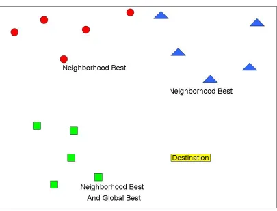
3.7 Particles in the swarm are moving randomly toward their destination . . . 30

3.8 Particles are getting closer to the best position of the neighborhood . . . 31

3.9 Particles are getting closer to the best global position . . . 32

4.1 Pseudocode for fluoroscopic analysis in the simplest form . . . 35

4.2 Pseudocode for sequential bees algorithm . . . 36

(15)

4.6 Pseudocode for parallel bees algorithm, Ctd . . . 40

4.7 Pseudocode for parallel PSO . . . 41

4.8 Pseudocode for parallel PSO, Ctd . . . 42

4.9 Program execution . . . 44

4.10 Config file for bees algorithm . . . 45

4.11 Config file for PSO . . . 46

5.1 Communication visualization for the parallel bees algorithm . . . 52

5.2 Communication visualization for the parallel PSO method . . . 53

(16)

CT– Computer Tomography

DRR– Digital Reconstructed Radiograph SI– Swarm Intelligence

PSO– Particle Swarm Optimization ACO– Ant Colony Optimization SDS– Stochastic Diffusion Search

(17)

CHAPTER 1 INTRODUCTION

1.1 Fluoroscopic Analysis

A good understanding of knee joint kinematics is essential for evaluating and researching the problems associated with the joint. To understand knee joint kinematics, determination of the position of the bones in the joint during motion in three dimensions is required. Flu-oroscopy is a medical imaging technique that produces real-time, two dimensional images of an object, whereas, computer tomography (CT) is an imaging technique that produces static three dimensional image of the scanned object. The two dimensional fluoroscopy frames and the three dimensional CT scan images are not individually sufficient to provide complete information about the position of the bones in the joint in motion as a function of time. However, three dimensional position data over time can be derived using the static CT scan images and real-time information from video fluoroscopy images together.

(18)

dimensions: x, y, andz. The film can rotate while the X-ray source can move in azimuth and elevation dimensions. This simulation is illustrated in Figure 1.1. The projection of the X-rays from the simulated source onto the film through the CT cube produces a DRR image. Different values of the X-ray source’s azimuth and elevation, the film’s rotation and the cube’sx,y, andzco-ordinates generate different DRR images. If a generated DRR image matches the fluoroscopy frame, the position of the cube, and the orientation of the X-ray source and the film are known. Using this information, a three dimensional rendering of the joint in motion can be constructed.

Figure 1.1: Geometric configuration of the simulated fluoroscope [1]

(19)

includ-ing generatinclud-ing DRR images, extractinclud-ing the edges of DRR images, and comparinclud-ing the edge images. These algorithms are based on the work of several researchers [2, 3]. Previous experiments used a Monte Carlo search technique to search for the matching DRR image, given an X-ray fluoroscopy image [1]. These experiments were conducted to search for azimuth and elevation of the camera and the rotation of the film. They have demonstrated that this can be achieved to an accuracy of 0.5 degree rotation, azimuth and elevation. The process, however, is very time consuming and calls for advanced search algorithms to reduce the time taken for finding the orientation of the X-ray source, the X-ray film and the position of the bones. This thesis uses swarm intelligence techniques in a parallel computing environment to achieve faster results.

1.2 Swarm Intelligence in a Parallel Computing Environment

Swarm intelligence is a branch of artificial intelligence based on the behavior of a group of entities working together to solve a common problem. “It is based on the collective behav-ior of decentralized, self-organized systems” [15, 26].” Swarms move through the search space and their collective intelligence leads the to the solution. Ant colony optimization (ACO), bees algorithm, particle swarm optimization (PSO), and stochastic diffusion search (SDS) are some of the techniques that exhibit swarm intelligence [5, 9, 11, 13]. These tech-niques have been used in many optimization problems like the traveling salesman problem, telecommunications routing, factory scheduling, etc. Swarm intelligence techniques are known to be robust and easy to implement.

(20)

technique based on the food foraging behavior of a swarm of honey bees [29, 30]. The bees in the group are divided into scout bees and worker bees. Scout bees go on a random search for flower patches and come back to the bee hive to report their findings. The quality and distance of each of the flower patches found is evaluated. Finally, the best ones are chosen and worker bees are sent to them to collect nectar. The second algorithm used in this thesis, the particle swarm optimization technique, is influenced by the flocking behavior in birds [33]. It consists of several particles organized into close knit groups or neighborhoods. The particles move in the search space searching for the destination by interacting with one another and they collectively arrive at the destination. It is based on the communication and interaction among particles which re-calculate their position and velocity values accordingly and move through the search space to find the solution [32].

(21)

1.3 Prior Research

This thesis is an extension to the research done by Scott et al. [1]. The goal of the research conducted by Scott et al. was to develop a method for collecting accurate, real time three dimensional kinematic data of bones and joints using two dimensional X-ray images resulting from a video fluoroscopy technique combined with the static three dimensional Computer Tomography data [1]. The process used in their research involved creating virtual X-rays from the CT image through the digitally reconstructed radiograph projections. Traditional methods used to achieve kinematic data of the joints require human intervention to initialize the starting position. The method they proposed was minimally invasive and used a Monte Carlo search technique with a variable search range. The search range decreased as matching between the target image and the image created with known position values improved. This was an optimization search. This is a very efficient method for small ranges of postion values.

Considering the extent of the allowed movement of the knee joint within the fluoroscope and the allowed width of the angular movements of the X-ray source and the X-ray film, the potential range of the position values is enormous. Therefore, this calls for an efficient search algorithm that is very fast in finding the values required. The purpose of the research in this undertaking is to find suitable parallelized search mechanisms to speed up the process of determining the three dimensional position data of the bones and joints using the same image processing techniques that were used by Scott et al.

1.4 Thesis Statement

(22)

(23)

CHAPTER 2 ALGORITHMS USED FOR FLUOROSCOPIC ANALYSIS

In this chapter, the meaning of fluoroscopic analysis and the algorithms used in the analysis are discussed.

2.1 Fluoroscopy

(24)

(25)

2.2 Computer Tomography

Computer Tomography (CT) is a medical imaging technique that uses X-rays. It is based on the concept of tomography. “The word ’tomography’ is derived from the Greek tomos (slice) and graphein (to write)” [22]. This means a series of slices or cross sectional images are stacked together to construct a three dimensional model of the object being scanned. These images are processed using a computer and several individual images for each slice are created. After completing all the required processing of these images, a detailed three dimensional picture of the internal structure of the body part that was scanned can be obtained. Figure 2.2 shows a modern CT scanning equipment. The patient is placed on the horizontal surface and the scanner takes cross sectional images and computes a CT scan image of the required body part [17].

A CT scan can be used to study many organs and parts of the human body [18]. A CT scan image of knee joint can be helpful in diagnosing the problems in the kinematics of the knee joint and can be useful in the placement of an artificial implant. An example of a CT scan is shown in Figure 2.3, which is a CT scan image of a knee joint.

2.3 Knee Joint Kinematics

(26)

(27)

Figure 2.3: CT scan of a knee joint [20]

(28)

Figure 2.4: Anatomy of a knee [19]

(29)

2.4 Fluoroscopic Analysis

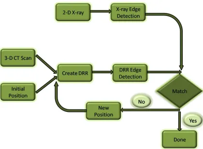
The process of determining three dimensional position data over time can be achieved using 3-D CT data and 2-D fluoroscopy images. This process is called fluoroscopic analysis. There are several steps required in this process. Figure 2.5 provides a block diagram of the major steps involved.

Figure 2.5: Procedure for fluoroscopic analysis

(30)

theazimuthandelevationof the X-ray source and thirdly, by therotationof the X-ray film about a central axis. The knee joint can also change its azimuth, elevation and rotation values, but in this experiment, those values for the joint are kept constant, while the film and the X-ray source are rotated instead. Thus, values of the six dimensions have to be measured over time in order to obtain the real-time positional information of the knee joint. Using the static CT scan image as input, the 3-D real time position data of the knee joint is constructed. In the first step, virtual X-ray images of the joint at different positions are created using the CT data. Then, the essential features of the image which are useful to determine the position are extracted. The essential features of the target X-ray frame from the fluoroscopy video images are also extracted. In the next step, the virtual image is compared with the target image. This process continues until there is a match. A match indicates the position of the joint for the first target fluoroscopy image. The whole process must be repeated for each fluoroscopy image in the video.

This process provides a rendering of the 3-D positional data over time. Sections 2.4.1 to 2.4.4 provided details for each of the above steps.

2.4.1 DRR Image Creation

(31)

the intersections yields the radiological path and attenuation. The ray tracing mechanism employed here is similar to the ray tracing used in computer graphics to generate 3-D images. But in computer graphics, the reflection or the path of the light rays off the pixels is used to generate the image, whereas, in fluoroscopic analysis, the transmittance of the X-rays to the film is used to generate the DRR image.

2.4.2 Edge Detection

Edge detection of an image is used to “identify points in the image at which the image brightness changes sharply or more formally has discontinuities” [23]. By applying an edge detector to an image, the amount of information contained in the image can be significantly reduced by filtering out the less relevant information and retaining only the structural properties of the object in the image. Using edges for comparison increases the probability of finding a match between a DRR image and a fluoroscopy image, as opposed to the comparison of the images themselves whose X-ray intensities may not match. This also decreases the amount of data to be processed and thus significantly simplifies the computations that involve interpreting the information contained in the image. In our implementation, Sobel’s edge detection method is used [4, 24]. This method finds the edges in an image using the gradient filter method.

(32)

-1 0 +1 -2 0 +2 -1 0 +1

+1 +2 +1

0 0 0

-1 -2 -1 Figure 2.6: Sobel Gx and Gy masks

are shown in Figure 2.6. TheGxmask highlights the edges in the horizontal direction and the Gy mask in the vertical direction. After taking the magnitude of both, the resulting output detects the edges in both directions.

The magnitude of the gradient is calculated using

|G|=pGx2₊_Gy2_. _(2.1)

An approximate magnitude can be calculated using

|G|=|Gx|+|Gy|. (2.2)

2.4.3 Image Matching

(33)

obtained by multiplying the two images together pixel by pixel and summing the result and then normalizing by the sum of the predicted image. IfJ(x,y) is the input contour image and K(x,y) is the predicted contour image, then contour match score (CMS) is calculated using

CMS= Σ(x,y)J(x,y)K(x,y)

Σ_(x,y)K(x,y) . (2.3)

2.4.4 Searching

The position of the knee joint is defined by six values, viz., the x, y, and z co-ordinate values and the azimuth, elevation and rotation values. Since each of these values has a large range, a simple brute force method of searching is highly inefficient. Each iteration of the search is a time-consuming process, because it involves creating a virtual image with known position values using ray tracing, extracting the edges and comparing it to the target image. Therefore, the goal should be to reduce the number of iterations of the search as well as the range of search with each iteration.

The measurement of the actual fluoroscope gives the range of values possible for each of the six positional parameters. The azimuth values of the X-ray source can range from -180 to +180 degrees and the elevation can be anywhere between -90 to +90 degrees. The film can rotate from -90 to +90 degrees. The knee joint or the hypothetical CT cube that is used in our experiments has a wide range of translation possible. Typically the object being scanned is placed close to the center and hence, for the tests conducted in this project, -5cm to +5cm translations from the center, on each axis, are considered.

(34)

remaining permutations is still dramatically large. And moreover, there is simply no way to sort the values for any of the six parameters due to the nature of the comparisons performed in the search. All search algorithms involve comparisons of the elements being searched for in one way or another. In this case, we compare two images and the matching algorithm used for this comparison produces a match score between 0 and 1 for each comparison. The values of the six positional parameters are known when the score is 1. The images are being compared and not the six values. There is no easy way to sort the images in any manner. Thus, this indicates that the usage of any search algorithm that depends on sorted elements is ruled out.

(35)

CHAPTER 3 SEARCH ALGORITHMS

In Chapter 2, the necessity of an efficient search algorithm in fluoroscopic analysis was explained. This chapter provides details of the algorithms adopted in this thesis. In addition to the Monte Carlo method that was used in prior research, the two SI techniques used in this thesis, the bees algorithm and particle swarm optimization, are presented here.

3.1 Monte Carlo Search Technique

The Monte Carlo search method is a non-deterministic method that depends on random sampling. The Monte Carlo method is generally used to solve problems that are difficult to solve using deterministic methods [14, 25]. This method solves problems by generating random numbers in each try. After evaluating each of these trials, it can be predicted if the solution has been reached or not, or if the system is getting closer to the solution. Monte Carlo methods have been heavily used in a wide variety of fields ranging from economics to nuclear physics.

(36)

1. Initialize the current parameter value to zero.

// This current value is evaluated based on the expected // target value in each iteration.

2. While (stopping criterion not met)

3. Generate random values and add it to the initial value. 4. Evaluate the fitness of the value obtained in step 3. 5. Negate the random values and add it to the current value. 6. Evaluate the fitness of the value obtained in step 5. 7. Select the better of the two values.

(This becomes the current value) 8. End While.

Figure 3.1: The pseudocode for the Monte Carlo search algorithm

arbitrary values generated using a random number generator. Random step values with a range of 0 to 10o are generated for each iteration of the search. Two sets of orientation values are obtained by adding and subtracting the step values to the initial values. DRR images are then generated using both these sets. A contour match score is calculated for the comparison of each of these images with the edge image of the target fluoroscopy frame. The parameter values that produce a better score is retained and the path that is more promising is chosen. Figure 3.1 gives the pseudocode for the Monte Carlo search algorithm.

The search continues by producing two new sets of random steps, which are added and subtracted to the current values obtained from the previous iteration. This cycle is repeated until a match is found and the score of the match is greater than 0.8. Thus, in each iteration of the search, the search space decreases and the search gets closer to the solution. This results in values that are approximately equal to the desired values.

(37)

that is close to the solution and hence the next stage of the search is expected to obtain a more accurate solution by searching in smaller steps. After both the stages are completed, the resulting parameter values should be fairly accurate. The sequential implementation of this method has been able to generate values within 0.5oof the desired parameter values.

3.2 Swarm Intelligence

The wordSwarm means a group of insects that are close to one another and engaged in a common activity. In general, swarmis a term used to describe the behavior of a group of animals that are similar to one another. Swarming behavior can be observed in many animals such as bees, ants, other insects, fish, bacteria and even people. This phenomenon can be called by different names such as flocking in birds, schooling in fishes, societal behavior in human beings and growth of colonies in bacteria.

Swarm intelligence is a phenomenon, based on self-organization, in which the group of insects or other beings solve complex problems together. The swarm arrives at the solution collectively. Constant and consistent communication and feedback among the group, and adherence to common rules are essential to the success of the swarm. Errors and randomness are the pillars of this system. Even if a few individuals fail to achieve their objective, the group as a whole can succeed. Examples of this behavior can be observed in the food foraging behavior in ants and bees, and migration in birds and fishes. Chances of foraging food, finding mates, avoiding predators, overcoming obstacles, migrating to a better place are made faster and easier by swarm intelligence. Swarm intelligence has a strongly noticeable benefit for all the members of the swarm.

(38)

co-operation among entities in a system is the key to solving a problem. The expression Swarm intelligence (SI) was introduced by Gerardo Beni and Jing Wang in 1989 in the context of cellular robotic systems [15]. There are several SI techniques such as the ant optimization algorithm, bees algorithm, particle swarm optimization, and stochastic diffu-sion search. SI techniques can be applied in problems involving finding the shortest path, swarm-based data analysis, robotics, financial forecasting, search, network management, Internet server optimization, etc. SI methods generally have simple rules and are easy to implement.

(39)

worked on by individual entities in the population. An entity is expected to communicate with every other entity in the system. This leads to significant communication overhead and is therefore not very suitable for parallel implementation.

The two SI techniques chosen to solve the search problem in fluoroscopic analysis are bees algorithm and particle swarm optimization. The group of entities in both methods can be easily mapped to processes in a parallel computing system. In addition to being easily parallelizable, they are also easy to implement. Sections 3.2.1 and 3.2.2 describe these two methods in depth.

3.2.1 Bees Algorithm

The bees algorithm [5, 29] is inspired by the behavior of a honey bees working together to find the sources of nectar, collecting it and storing it back in their hives. It is a population-based search algorithm [5]. This approach has been used to solve many optimization problems.

(40)

the flower patch. Figure 3.2 depicts the bee waggle dance. All the scout bees perform the waggle dance after returning from the flower patches. After learning about the distance and quality of all the flower patches through the waggle dances, the flower patches are evaluated based on some criteria. A few best sites are chosen from these if their fitness value is above a certain threshold. A large number of worker bees are recruited to collect nectar from the most promising sites and the remaining worker bees are sent to the other flower patches. Sites that are very far and those that have very few flowers with nectar and pollen are discarded. The scout bees are sent again in search of new flower patches for the next round.

(41)

1. Initialize the population with random solutions. 2. Evaluate fitness of the population.

3. While (stopping criterion not met) //Forming new population.

4. Select sites for neighborhoods search. 5. Recruit bees for selected sites

(more bees for best e sites) and evaluate fitnesses.

6. Select the fittest bee from each patch. 7. Assign remaining bees to search randomly

and evaluate their fitnesses. 8. End While.

Figure 3.3: The pseudocode for the bees algorithm in its simplest form [6]

The bees algorithm in its simplest form requires a number of parameters [6], namely:

1. number of scout bees (n)

2. number of sites selected out ofnvisited sites (m)

3. number of best sites out ofmselected sites (e)

4. number of bees recruited for bestesites (nep)

5. number of bees recruited for the other (m-e) selected sites (nsp)

6. initial size of the patches (ngh)

7. stopping criterion

The pseudocode is presented in Figure 3.3.

(42)

can also be more than one way to reach a flower patch. In Figure 3.5, the returning scout bees perform the waggle dance in the bee hive and as a result of this the majority of the worker bees fly to the larger and closer sites via the shortest route. Scout bees go in search of new sites.

Figure 3.4: Food foraging in bees - scout bees are going in search of flower patches

3.2.2 Particle Swarm Optimization

(43)

(44)

network and depends on a communication structure in the network. Just as a person benefits from his interaction with society, a particle in the swarm enhances its position in the system due to its interaction with other particles. People in a society talk to other people to find out their experiences, and try to solve their problems using the inputs given by others. Other people’s views and attitudes might affect an individual’s own opinions and future decisions. Some people are more influential than the others. There are various factors that can affect the social dynamics such as who the neighbors are, how they influence the direction an individual takes in his journey to a destination and his own progress at any moment.

Particle swarms are used to simulate social networks as well as several engineering applications. Particle swarm optimization techniques can be used in search problems, where the particles in the swarm communicate with one another and reach the solution faster than they would have if they were on their own. This technique has also been used to address other complex optimization problems, pattern recognition, data mining and image processing.

(45)

1. Initialize the particle positions and velocities. 2. While (global best value does not match solution) 3. Move particle to a random position from the current

position within a certain threshold from the current position.

4. Store the local best value.

5. Talk to neighbors and exchange neighborhood search information.

6. Store neighborhood best value. 7. Store global best value.

8. Update position and velocity to the neighborhood best. 9. End While.

Figure 3.6: The pseudocode for the general PSO [32]

a particle designated in every neighborhood to keep track of the best global value. The particles adjust their postions at regular intervals based on the best local, neighborhood and global values. Thus they move towards those particles in their neighborhood, that have the best fitness values. Over time they converge toward good positions and move about in the search space in close proximity to the best global value and stop exploring the rest of search space. The rest of the search space, which has a very low likelihood of containing the solution, is discarded. The pseuodocode that explains this technique is given in Figure 3.6.

(46)

toward the neighbor with the best fitness value. In ideal cases, after several iterations of this exercise, the particles converge toward the best global fitness value and thus converge to the solution. This stage looks similar to what is shown in Figure 3.9. All the particles then begin to search intensively around the best value until they find the solution.

Figure 3.7: Particles in the swarm are moving randomly toward their destination

(47)

(48)

(49)

CHAPTER 4 DESIGN AND IMPLEMENTATION

The search problem involved in the fluoroscopic analysis process has been decribed in Chapter 1. While Chapter 2 provided an introduction to the world of fluoroscopic analysis and presented the computing problems associated with the process, Chapter 3 presented different methods to solve the search problem in fluoroscopic analysis. In this chapter, the design and implementation details as well as the pseudocode for the bees algorithm and particle swarm optimization method used for this thesis are provided.

4.1 Design Approach

(50)

The second step consisted of developing a good organization structure and an activity flow-chart, which are very essential to a good design. All the steps involved in the process were studied. Each step required an separate component. For fluoroscopic analysis, different components are required for specific tasks, such as, generating DRR images from a given postion and a CT scan image, image filtering for extracting the edges of an X-ray or DRR image, image matching, and fluoroscopic searching. Figure 2.5 in Chapter 2 provides an activity flow-chart for fluoroscopic analysis that illustrates the different stages in the fluoroscopic analysis and the steps to transition from one stage to another.

The third step involved identifying the different entities in the system and designing data structures for each of them. The main entities are:

1. CT Volume - used to represent a CT scan image.

2. DRR Image - used to represent a DRR X-ray image.

3. Bee - used to represent a bee in bees algorithm.

4. Particle - used to represent a particle in PSO method.

5. Sobel filter kernels - used in the Filtering method to extract edges of an X-ray image

These data structures are presented in Appendix B.

(51)

Fluoroscopic Analysis(CTCube, TargetXrayImage)

1. TargetEdges = SobelFilter(TargetXrayImage) 2. score = 0

3. While(score < GOOD_MATCH_SCORE) 4. x = Random()

5. y = Random() 6. z = Random()

7. azimuth = Random() 8. elevation = Random() 9. rotation = Random() 10. TestDRRImage =

GenerateDRR(CTCube,x,y,z,azimuth,elevation,rotation) 11. TestEdges = SobelFilter(TestDRRImage)

12. score = ContourMatching(TestEdges, TargetEdges) 13. Match found.

Position values are x, y, and z.

Orientation values are azimuth, elevation, and rotation

Figure 4.1: Pseudocode for fluoroscopic analysis in the simplest form

4.2 Build Infrastructure

Build infrastructure provides the capability to add new code to the project, compile and maintain the code. The project files are organized in such a manner that it facilitates the ease of compiling and executing the application. All the code and the input files are placed in a repository controlled by a version control system called Subversion. The main makefile is placed in the main directory of the project. This makefile facilitates all the build actions required for the project. The makefile targets and the functions performed by them are given in Appendix A.

(52)

Sequential_Bees(CTCube, TargetXrayImage)

n = Number of bees

m = Number of best sites

p = Number of bees chosen for the best sites (best bees) q = n-p = Number of bees chosen as scout bees for the next

iteration

r = Number of individual bee iterations

1. TargetEdges = EdgeFilter(TargetXrayImage) 2. While(BestScore < GOOD_MATCH_SCORE): 3. Foreach Bee:

4. For i = 0 to p: 5. if(scout bee)

//In the first iteration of #1, all bees are //scout bees

6. Generate random values for position(x,y,z) and orientation(az,el,rt)

7. else if(worker bee)

8. Generate random step values and add them to the previous values.

9. TestDRRImage = GenerateDRR(x,y,z,az,el,rt, CTCube) 10. TestEdges = EdgeFilter(TestDRRImage)

11. BeeScore = ContourMatching(TestEdges,TargetEdges) 12. BeeScore = Calculate best of all the p scores

//Waggle dance section

13. Rank the BeeScore of all the individual bees

14. Choose the m best sites from the list based on scores. 15. Assign p bees to m sites equally (worker bees)

16. Assign q bees for random search (scout bees)

17. Save the BestScore and the values associated with it 18. End While

19. [x,y,z,az,el,rt] associated with BestScore

are the required position and orientation values. 20. End

(53)

Sequential_PSO(CTCube, TargetXrayImage)

n = Number of particles m = Number of neighborhoods

p = Number of particles in a neighborhood r = Number of individual particle iterations

1. TargetEdges = EdgeFilter(TargetXrayImage) 2. Foreach neighborhood m:

3. NeighborhoodBest = 0.0 4. GlobalBest = 0.0

5. While(BestScore < GOOD_MATCH_SCORE): 6. Foreach Neighborhood m:

7. if NeighborhoodBest < 0.1:

//This means, search randomly 8. RANDOMSTEP = 0

9. else if NeighborhoodBest < 0.4

//Add large random steps to previous value 10. RANDOMSTEP = LARGESTEP

//Add medium random steps to previous value 12. RANDOMSTEP = MEDIUMSTEP

//Add small random steps to previous value 14. RANDOMSTEP = SMALLSTEP

(54)

15. Foreach neighbor p: 16. For i = 0 to r: 17. if(RANDOMSTEP == 0):

//In the 1st iteration all particles //search randomly

19. else:

20. Generate random step values and

add them to the previous neighborhood best values.

21. TestDRRImage =

GenerateDRR(x,y,z,az,el,rt, CTCube) 22. TestEdges = EdgeFilter(TestDRRImage) 23. ParticleScore =

ContourMatching(TestEdges,TargetEdges) 24. ParticleBestScore =

the best of all the r particle scores 25. NeighborhoodBest =

the best of all scores in the neighborhood 26. GlobalBest = the best of all scores

27. End While

28. [x,y,z,az,el,rt] associated with GlobalBest

(55)

Parallel_Bees(CTCube, TargetXrayImage)

n = Number of bees/processes m = Number of best sites

p = Number of bees chosen for the best sites (best bees) q = n-p = Number of bees chosen as scout bees for the

next iteration

r = Number of individual bee iterations

1. TargetEdges = EdgeFilter(TargetXrayImage)

2. Barrier() //Wait for all processes to arrive at this point 3. While(BestScore < GOOD_MATCH_SCORE):

4. Foreach Bee:

5. For i = 0 to p: 6. if(scout bee)

//In the first iteration of #1, all bees are //scout bees

8. else if(worker bee)

9. Generate random step values and add them to the previous values.

10. TestDRRImage = GenerateDRR(x,y,z,az,el,rt,CTCube) 11. TestEdges = EdgeFilter(TestDRRImage)

12. BeeScore = ContourMatching(TestEdges,TargetEdges) 13. BeeScore = Calculate best of all the p scores

(56)

//Waggle Dance section 14. if( process_id != 0):

//All processes other than process 0,

//send their scores and 6 value to process 0 15. Send(BeeScore,x,y,z,az,el,rt) to Process 0 16. else if(process_id == 0):

17. for(i =1 to n):

18. Recv(BeeScore,x,y,z,az,el,rt) from Process i

19. Rank the BeeScore of all the individual bees 20. Choose the m best sites from the list based on

scores.

21. Save the BestScore and the values associated with it

22. for(i=1 to n):

//Send information about best sites to the // best bees. Make some bees random.

23. Send(BeeScore, x,y,z,az,el,rt,ScoutOrWorkerFlag) to Process i.

24. if(process_id != 0)

25. Recv(BeeScore, x,y,z,az,el,rt,ScoutOrWorkerFlag) from Process 0

26. End While

27. [x,y,z,az,el,rt] associated with BestScore

(57)

Parallel_PSO(CTCube, TargetXrayImage)

n = Number of particles/processes

Every particle in the system has a particle_id m = Number of neighborhoods/process groups

p = Number of particles in a neighborhood

Every neighbor in a neighborhood has a neighbor_id r = Number of individual particle iterations

1. TargetEdges = EdgeFilter(TargetXrayImage) 2. Create m ProcessGroups //Neighborhoods

3. Initialize all neighbors in a group/neighborhood 4. GlobalBest = 0.0

5. Barrier() //Wait for all particles to get initialized 6. While(BestScore < GOOD_MATCH_SCORE):

//This is done by all neighborhoods. 7. if NeighborhoodBest < 0.1:

8. RANDOMSTEP = 0 //This means, search randomly 9. else if NeighborhoodBest < 0.4

10. RANDOMSTEP = LARGESTEP

//Add large random steps to previous value 11. else if NeighborhoodBest < 0.6

12. RANDOMSTEP = MEDIUMSTEP

//Add medium random steps to previous value 13. else if NeighborhoodBest < 0.8

14. RANDOMSTEP = SMALLSTEP

//Add small random steps to previous value 15. For i = 0 to r:

16. if(RANDOMSTEP == 0):

//In the 1st iteration all particles search randomly 17. Generate random values for position(x,y,z)

and orientation(az,el,rt) 18. else:

19 Generate random step values and

add them to the previous neighborhood best values 20. TestDRRImage = GenerateDRR(x,y,z,az,el,rt, CTCube) 21. TestEdges = EdgeFilter(TestDRRImage)

22. ParticleScore= ContourMatching(TestEdges,TargetEdges) 23. ParticleBestScore= the best of all the r particle scores

(58)

24. if(neighbor_id != 0):

//All neighbors send their score //and values to neighbor with id=0 25. Send(ParticleBestScore, x,y,z,az,el,rt)

to neighbor 0 26. else:

//neighbor 0 receives all the scores 27. for( i=1 to p):

28. Recv(ParticleBestScore, x,y,z,az,el,rt) from neighbor i

29. Store the NeighborhoodBest score

//Send the neighborhood best score and //values back to others

30. for( i=1 to p):

31. Send(NeighborhoodBest, x,y,z,az,el,rt) to neighbor i

32. if(neighbor_id !=0):

33. Recv(NeighborhoodBest, x,y,z,az,el,rt) from neighbor 0

34. if(particle_id != 0):

35. Send(NeighborhoodBest, x,y,z,az,el,rt) to particle 0

36. else:

37. for( i=1 to n):

38. Recv(NeighborhoodBest, x,y,z,az,el,rt) from particle i

39. Store the GlobalBest score 40. End While

41. [x,y,z,az,el,rt] associated with GlobalBest

(59)

A.

4.3 Implementation Details

Implementation of this application consists of several files of C code that implement all the algorithms required for each step in fluoroscopic analysis. The inputs to this application are DRR images of pre-determined postions and orientation or an actual 2-D X-ray fluo-roscopic frame as the target images, CT scan image, and configuration files that describe the parameters required to define the algorithms. The program outputs the position and orientation of the best matching score. By configuring the makefile to generate the debug version of the program, the program can be made to print out more information about each iteration of the search.

The algorithms are implemented as library plugins that can be dynamically linked to the main program. The main program performs all the main steps of extracting the CT volume information from the input CT image, and making dynamic calls to the required libraries for each of the other functions such as searching, generating DRR, etc. By implementing the algorithms as dynamically linked plugins, the flexibility for using any algorithm for a specific task is provided. This makes it possible to implement a new algorithm for any step and compile it independently. No changes are needed to any other part of the project to use the new plugin. The new plugin has to only be specified as a parameter while executing the application. This is done to allow further research and experimentation for the fluoroscopic analysis and to make it easy to explore different possibilities of solving this problem.

(60)

Operating System Linux - CentOS release 5.2 Version Control System Subversion 1.4.2

Programming Language C

Libraries mpich2, nrutils

Sequential Compiler gcc

Parallel Compiler mpicc

Parallel Computing platform Beowulf cluster Scripting Language Korn Shell

Debugger gdb

Memory Profiler Valgrind

Table 4.1: Environment details

Execution of sequential program: fluoro_s

Execution of parallel program:

mpiexec -l -n <num of processes> fluoro_p <path to search plugin(.so lib file)> <path to the input config file>

Figure 4.9: Program execution

An example config files for the bees algorithm and the particle swarm optimization method is provided in Figures 4.10 and 4.11, respectively.

4.4 Test Infrastructure

(61)

#Input CT image

CT_IMAGE=<path>/images/really_small_cube.txt #Target DRR with known postion values

DRR_IMAGE=<path>/images/drr_image10_10_10_8_8_8.txt

GENERATE_DRR_LIB=<path>/lib/libp_generate_drr_raytracing.so FILTER_LIB=<path>/lib/libp_filter_sobel_bw.so

MATCH_LIB=<path>/lib/libp_match_contour_bw.so MAX_ITER=3

BEE_ITER=1 NUM_BEES=8 NUM_BEST_BEES=6 NUM_BEST_SITES=3 RANDOM_SEED=123

AZIMUTH_RANGE=180 #In degrees ELEVATION_RANGE=90 #In degrees ROTATION_RANGE=90 #In degrees TRANSLATION_RANGE=20 #In pixels TRANSLATION_FINE_STEP=3 #In pixels ORIENTATION_FINE_STEP=5 #In degrees

(62)

#Input CT image

CT_IMAGE=<path>/images/really_small_cube.txt #Target DRR with known postion values

DRR_IMAGE=<path>/images/drr_image10_10_10_8_8_8.txt

GENERATE_DRR_LIB=<path>/lib/libp_generate_drr_raytracing.so FILTER_LIB=<path>/lib/libp_filter_sobel_bw.so

MATCH_LIB=<path>/lib/libp_match_contour_bw.so MAX_ITER=3

PARTICLE_ITER=1 NUM_PARTICLES=8 NUM_NEIGHBORHOODS=4 RANDOM_SEED=123

AZIMUTH_RANGE=180 #In degrees ELEVATION_RANGE=90 #In degrees ROTATION_RANGE=90 #In degrees TRANSLATION_RANGE=20 #In pixels

TRANSLATION_FINE_STEP_LEVEL1=10 #In pixels TRANSLATION_FINE_STEP_LEVEL2=5 #In pixels TRANSLATION_FINE_STEP_LEVEL3=3 #In pixels ORIENTATION_FINE_STEP_LEVEL1=10 #In degrees ORIENTATION_FINE_STEP_LEVEL2=5 #In degrees ORIENTATION_FINE_STEP_LEVEL3=1 #In degrees

(63)

(64)

CHAPTER 5 TESTING AND RESULTS

The implementation details for the fluoroscopic analysis process and the test infrastructure developed are provided in Chapter 4. This chapter lists the efforts to test this implementa-tion.

5.1 Test Cases

Software implementations require thorough testing for verifying the code and also validat-ing the results obtained for the given inputs. Testvalidat-ing the implementation of fluoroscopic analysis process is required for the following purposes:

• To check the correctness of code by running it against various inputs and checking if the program runs to completion successfully.

• To verify if the parallel implementation does generate the required output in shorter time compared to the sequential implementation.

• To find the better of the two SI methods, bees algorithm and particle swarm opti-mization, for solving the search problem in fluoroscopic analysis.

(65)

the two versions. Several test cases are designed to test the implementation to enable the verification of all the the points mentioned above.

The implementation for the bees algorithm and the particle swarm optimization al-gorithm require several parameters to be set to successfully initialize the system. The bees algorithm requires values for the number of bees, number of best sites to choose, the number of bees to allocate to each best site, etc. In the case of particle swarm optimization, the set of parameters include the number of particles, number of neighborhoods and number of members in a neighborhood. These parameter values are placed in a configuration file and given as input to the main program. Examples of the configuration files for the Bees and particle swarm optimization algorithms are provided in Figures 4.10 and 4.11 respectively. In this project, different test cases are derived by specifying different parameters for each algorithm. Therefore, by creating several configuration files, one for each set of test configurations, many test cases are constructed.

An attempt has been made to diversify the parameters in such a way that the program will be tested for different sizes of the groups (bees or particles), different sizes of the sub-groups, different position and orientation values of the target image, and so on. This would help in the determination of an optimized combination of parameters. For example, a particle population consisting of 36 particles grouped into 6 neighborhoods of 6 members each, might give faster results than a population grouped into 12 neighborhoods of 3 members each. In the case of bees algorithm, if 3 best sites are chosen and 10 bees are selected for each of the 3 sites from a population of 36 bees, while allowing the remaining 6 bees to search randomly, the grouping might provide better results than any other grouping of the bees.

(66)

another within their colony. Which method is more suitable for fluoroscopic analysis? How many entities are required for the search to provide optimal results without costing any severe communication overhead? What is an ideal grouping of the entities involved? Do smaller number of groups with large sizes work better than larger numbers of groups with small sizes? What kind of target images result in good solutions? Does the implementation provide good results only for a small subset of the target images or does it hold for any range? The execution of tests attempts to answer these question that help determine the limitations and strengths of each algorithm by configuring several permutations and combinations of the parameter values. Tables 5.1 and 5.2 provide some of the test cases for the bees algorithm and the particle swarm optimization method respectively. Additionally, these combinations are executed multiple times with different target DRR images and for several number of maximum iterations.

Configuration/ Testcase 1 2 3 4 5 6 Number of Bees 12 24 24 24 36 36 Number of Best Bees 9 20 18 16 27 30 Number of Scout Bees 3 4 6 8 9 6

Number of Best Sites 3 2 6 4 9 6 Table 5.1: Test Cases for bees algorithm

Configuration/ Testcase 1 2 3 4 5 6 Number of Particles 12 24 24 24 36 36

Number of Neighbors 4 6 4 3 4 6

Number of Neighborhoods 3 4 6 8 9 6 Table 5.2: Test Cases for PSO

(67)

visualize the communication in terms of send and receive operations between the pro-cesses by reading those logs. Figure 5.1 provides the visualization of the inter-process communication during the execution of bees algorithm. The left pane of the picture lists the 12 processes with id 0 to 11. The timeline is seen at the bottom pane. It can be noted that for each iteration, all the bees or processes send their values to the master process (id = 0) and the master process sends a value after comparison and evaluation of all sent values, back to all the bees. This cycle repeats for every iteration of the search. The inter-process communication for particle swarm optimization algorithm is quite different from this. Figure 5.2 provides the visualization for this communication. In this, it can be seen that in each iteration, subgroups communicate among themselves first, where all the subgroup members send message to and receive from the subgroup leader. The leaders then communicate with the master process. The communication overhead load on the master process is much lesser in the case of particle swarm optimization than bees algorithm. Considering the time taken for each iteration in generating a DRR image and comparing that to a target DRR image, the communication overhead caused by sending and receiving matching score values at the end of each iteration is not very significant.

5.2 Results

(68)

(69)

(70)

the number of processes, then the time taken forniterations reduces by a factor ofn/p. Of course, the actual value will be less than this if we account for the process communication overhead.

Mode of Algorithm Max Number of Time Taken Speed Up Execution Iteration Entities (in secs)

Sequential Bees 100 12 1161.554

Parallel Bees 100 12 104.893 11.07

Sequential PSO 100 12 1183.173

Parallel PSO 100 12 104.777 11.29

Table 5.3: Timing results

All the experiments confirmed that the the time taken by the parallel programs were less than the time taken by their sequential counterparts by a significant amount. One such instance is provided in Table 5.3.

These results help in verifying the first test objective and part of the second objective. The sequential and parallel programs have run without any crashes or execution errors for all the configuration values for large number of iterations. In addition, for the same number of iterations, the parallel programs are considerably faster than the sequential programs.

(71)

(72)

CHAPTER 6 CONCLUSIONS

6.1 Swarm Intelligence for Solving the Search Problem

Fluoroscopic analysis of knee joint kinematics consists of determining the position and orientation of the bones in the knee joint. In the experiments conducted in this thesis, a hypothetical fluoroscope with a CT cube placed between an X-ray camera and an X-ray film, is used. The objective of the thesis is to find the position of the CT cube and azimuth and elevation angles of the camera and the rotation of the film for a given CT scan image and a target fluoroscopy X-ray frame.

The focus of this thesis has been to develop faster search algorithms for finding the position and orientation information. This is done by implementing the two swarm intelligence techniques, the bees algorithm and the particle swarm optimization method, for sequential and parallel execution. Both these methods are biologically inspired algorithms. While the bees algorithm mimics the food foraging behavior of the bees, particle swarm optimization method is inspired by the social behavior of a flock of birds or a school of fish. By adopting the communication and collaboration among a population of entities to solve a common problem, it is easier to reach a better solution faster.

(73)

method are easily parallelizable and are easy to apply to a problem of this nature. The experiments conducted to test the implementation provide sufficient information to indicate that parallel computing can significantly decrease the time required to search the position and orientation values in the fluoroscopic process. Several configurations of the bees and the particle swarm optimization algorithms have been successfully executed.

6.2 Future Scope

There is scope for further research in several components of the fluoroscopic analysis process. In order to derive accurate results, it is essential to have very efficient and effective methods for each of the analysis operations such as the DRR image generation, filtering of essential information from DRR or X-ray images, matching two DRR or X-ray images as well as searching for the position and orientation values from a given CT image and a target X-ray image. While the bees and particle swarm optimization algorithms appear to be promising solutions to the search problem, more analysis has to be carried out to find the best configuration to get optimum results out of these two methods, and this would be possible with accurate results from the other steps in the fluoroscopic process.

(74)

BIBLIOGRAPHY

[1] Scott, C and Barney Smith, E. H. An Unsupervised Fluoroscopic Analysis of Knee Joint Kinematics.IEEE Computer Society Washington, DC, USA, 2006.

[2] Siddon, R. L. Fast calculation of the exact radiological path for a three-dimensional CT array.Medical Physics 12(2), Mar/Apr 1985, pp. 252-255.

[3] Sarojak, M., Hoff, W., Komistek, R, and Dennis, D. An Interactive System for Kinematics Analysis of Artificial Joint Implants. Proc. of 36th Rocky Mountain Bioengineering Symposium, Copper Mountain, Colorado, 16-18 April 1999.

[4] Gonzalez, R. C., Woods, R. E.Digital Image Processing.Addison-Wesley Publishing Company, 1992.

[5] Pham, D. T., Ghanbarzadeh, A., Koc, E., Otri, S., Rahim, S., and Zaidi, M. The Bees Algorithm. Technical Note, Manufacturing Engineering Centre, Cardiff University, UK, 2005.

[6] Pham, D. T., Ghanbarzadeh, A., Koc, E., Otri, S., Rahim, S., and Zaidi, M. The Bees Algorithm - A Novel Tool for Complex Optimisation Problems.Proceedings of IPROMS 2006 Conference, pp.454-461.

[7] Von Frisch, K. Bees: Their Vision, Chemical Senses and Language. (Revised edn) Cornell University Press, N.Y., Ithaca, 1976.

[8] Kennedy, J. and Eberhart, R.Particle Swarm Optimization.Proceedings of the IEEE International Conference on Neural Networks, Perth, Australia, IEEE Service Center, Vol. 4. Piscataway, NJ, 1995, pp. 1942C1948.

[9] Parsopoulos, K.E., Vrahatis, M.N. Recent Approaches to Global Optimization Prob-lems Through Particle Swarm Optimization.Natural Computing, 1 (2-3), pp. 235-306, 2002.

[10] Clerc, M. Particle Swarm Optimization.ISTE, ISBN 1-905209-04-5, 2006.

(75)

[12] Dorigo, M., St¨utzle, T. Ant Colony Optimization.MIT Press. ISBN 0-262-04219-3, 2004.

[13] Bishop, J. M. Stochastic Searching Networks. Proc. 1st IEEE Conf. on Artificial Neural Networks, pp 329-331, London, 1989.

[14] Metropolis, N., Ulam, S.The Monte Carlo Method.Journal of the American Statisti-cal Association 44 (247): 335341, 1949.

[15] Beni, G., Wang, J.Swarm Intelligence in Cellular Robotic Systems.NATO Advanced Workshop on Robots and Bialogical Systems, Tuscany, Italy, 1989.

[16] University of Virginia Health System.World Wide Web.http://www.healthsystem.vir ginia.edu/uvahealth/adult radiology/fluoros.cfm

[17] Toshiba Medical Systems - Aquilion ONE.World Wide Web.http://www.toshiba-medi cal.eu/en/Our-Product-Range/CT/Systems/Aquilion-ONE

[18] WebMD.World Wide Web.http://www.webmd.com/a-to-z-guides/computed-tomogra phy-ct-scan-of-the-body

[19] ACL Solutions - Anatomy of the Knee.World Wide Web.http://www.aclsolutions.com /anatomy.php

[20] 64-CT Scan: Physician-Approved Information For Patients.World Wide Web.http:// www.64ctscan.com

[21] Wikipedia - Fluoroscopy.World Wide Web.http://en.wikipedia.org/wiki/Fluoroscopy [22] Wikipedia - X-ray computed tomography.World Wide Web.http://en.wikipedia.org/w

iki/X-ray computed tomography

[23] Wikipedia - Edge detection.World Wide Web.http://en.wikipedia.org/wiki/Edge dete ction

[24] Wikipedia - Sobel operator.World Wide Web.http://en.wikipedia.org/wiki/Sobel ope rator

[25] Wikipedia - Monte Carlo method.World Wide Web.http://en.wikipedia.org/wiki/Mont e Carlo method

[26] Wikipedia - Swarm Intelligence.World Wide Web.http://en.wikipedia.org/wiki/Swar m intelligence

(76)

[28] Scholarpedia - Stochastic Diffusion Search.World Wide Web.http://www.scholarped ia.org/article/Stochastic diffusion search

[29] Wikipedia - Bees Algorithm.World Wide Web.http://en.wikipedia.org/wiki/Bees algo rithm

[30] Wikipedia - Bee colony optimization.World Wide Web.http://en.wikipedia.org/wiki/ Bee colony optimization

[31] Wikipedia - Waggle dance.World Wide Web.http://en.wikipedia.org/Wiki/Waggle da nce

[32] Wikipedia - Particle Swarm Optimization.World Wide Web.http://en.wikipedia.org/ wiki/Particle swarm optimization

(77)

APPENDIX A

README FILE

---Readme file Fluoroscopy Project ---Sections: 1. Description

2. Steps Invloved in Executing the Project.

3. How to Compile the Project.

4. Makefile Features.

5. How to Run the Project.

6. Directory Structure of the Project.

7. How to Add a Plugin.

8. Code Documentation.

9. Naming Conventions.

10. Scripts. 11. Config Files. 12. Results.

13. Examples for Compiling and Executing the Project.

---1. Description

---This project performs an unsupervized fluoroscopic

analysis of knee-joint kinematics. The operations involved include

1. reading a CT scan image, 2. generating DRR images,

(78)

4. matching the edges of two different DRR images and having a score associated with it,

5. and searching for the right DRR image for a CT image, by using different combinations of the film and camera orientation and CT cube offsets.

---2. Steps Involved in Executing the Project

---The main program of this project relies on the

availability of shared libraries for the following operations : generating DRR, filtering, matching and searching. Below are a list of steps required to execute this project. Refer to relevant sections for details in each step. In order to use the Makefile provided as is, please follow the directory structure and the other requirements as mentioned for each step. Deviation from them would require custom makefiles or modification to paths in the makefile or whatever is required for the specific change.

1. Place the CT image file in the ’images’ directory. 2. Place a DRR image for that CT image in the ’images’

directory. The DRR image file for a CT image,

can also be created by running the program create_target_drr with the required camera and film orientation and cube offsets. Refer to section 3.A and 5.A.

3. Create an input config file which lists all the parameters required for running the program, such as number of iterations to run the search, path to the CT image, path to the DRR image, and any other parameters required for the algorithm chosen.

Place this file in the ’config’ directory. Refer

to section 3.E

4. Compile all the plugins required for the instance

of the program. Each plugin should be in a

(79)

5. Compile the main program by specifying the compiler. Refer to section 3.D.

6. Run the program by providing the input config file. Refer to section 5.B.

---3. How to Compile the Project

---$(FLUOROSCOPY) represents the path to the fluoroscopy project source, the outermost directory of the trunk, which consists of main makefile and all other

directories.

A. To compile the create_drr_image program: cd /$(FLUOROSCOPY)

make clean_create_drr make create_drr

B. To compile all the plugins in the ’plugins’ directory:

cd /$(FLUOROSCOPY) make clean_plugins make plugins

Note: This creates a .so file for sequential and parallel, for DOF=3 and 6, and all the permutations required.

DOF = Degrees of Freedom

C. To compile a single plugin:

For any plugin, you can run ’make clean’ followed by ’make all’ to make all libraries that are possible

for that plugin. To only make a particular library,

run make with required parameters.

D. To compile the main program: cd /$(FLUOROSCOPY)