Geosci. Model Dev., 8, 501–531, 2015 www.geosci-model-dev.net/8/501/2015/ doi:10.5194/gmd-8-501-2015
© Author(s) 2015. CC Attribution 3.0 License.
Development and basic evaluation of a prognostic aerosol scheme
(v1) in the CNRM Climate Model CNRM-CM6
M. Michou, P. Nabat, and D. Saint-Martin
CNRM-GAME, Météo-France, Centre National de Recherches Météorologiques, UMR3589, 42 avenue G. Coriolis, 31057 Toulouse CEDEX 1, France
Correspondence to: M. Michou ([email protected]) and P. Nabat ([email protected])
Received: 12 August 2014 – Published in Geosci. Model Dev. Discuss.: 25 September 2014 Revised: 26 January 2015 – Accepted: 3 February 2015 – Published: 9 March 2015
Abstract. We have implemented a prognostic aerosol scheme (v1) in CM6, the climate model of CNRM-GAME and CERFACS, based upon the GEMS/MACC aerosol module of the ECMWF operational forecast model. This scheme describes the physical evolution of the five main types of aerosols, namely black carbon, organic mat-ter, sulfate, desert dust and sea salt. In this work, we de-scribe the characteristics of our implementation, for instance, taking into consideration a different dust scheme or boost-ing biomass burnboost-ing emissions by a factor of 2, as well as the evaluation performed on simulation output. The simula-tions consist of time slice simulasimula-tions for 2004 condisimula-tions and transient runs over the 1993–2012 period, and are either free-running or nudged towards the ERA-Interim Reanaly-sis. Evaluation data sets include several satellite instrument AOD (aerosol optical depth) products (i.e., MODIS Aqua classic and Deep-Blue products, MISR and CALIOP prod-ucts), as well as ground-based AERONET data and the de-rived AERONET climatology, MAC-v1. The uncertainty of aerosol-type seasonal AOD due to model internal variabil-ity is low over large parts of the globe, and the character-istics of a nudged simulation reflect those of a free-running simulation. In contrast, the impact of the new dust scheme is large, with modelled dust AODs from simulations with the new dust scheme close to observations. Overall patterns and seasonal cycles of the total AOD are well depicted with, however, a systematic low bias over oceans. The comparison to the fractional MAC-v1 AOD climatology shows disagree-ments mostly over continents, while that to AERONET sites outlines the capability of the model to reproduce monthly climatologies under very diverse dominant aerosol types. Here again, underestimation of the total AOD appears in
sev-eral cases, sometimes linked to insufficient efficiency of the aerosol transport away from the aerosol sources. Analysis of monthly time series at 166 AERONET sites shows, in gen-eral, correlation coefficients higher than 0.5 and lower model variance than observed. A large interannual variability can also be seen in the CALIOP vertical profiles over certain re-gions of the world. Overall, this prognostic aerosol scheme appears promising for aerosol-climate studies. There is room, however, for implementing more complex parameterisations in relation to aerosols.
1 Introduction
502 M. Michou et al.: A prognostic aerosol scheme (v1) in CNRM-CM6 uneven distribution in the atmosphere remains hard to
simu-late with current climate models (Boucher et al., 2013). Although a community of global aerosol modellers has been working together for more than 10 years under the Ae-roCom project (Aerosol Comparisons between Observations and Models), with coordinated simulation exercises analysed in a large number of papers (see Kinne et al., 2006, and Tex-tor et al., 2006, as first papers, and http://aerocom.met.no for a list of publications), aerosol schemes within climate mod-els, such as those used for phase 5 of the Coupled Model Intercomparison Project (CMIP5, Taylor, 2009), are still un-dergoing development and evaluation (see e.g., Evan et al., 2014). Modelling requires a fundamental understanding of processes and their representation in large-scale models, and a number of climate models continue to consider prescribed aerosol climatologies. Such climatologies have been contin-uously upgraded, from Tanré et al. (1984) to Kinne et al. (2013).
More recently, the ACCMIP (Atmospheric Chemistry and Climate Model Intercomparison Project; Lamarque et al., 2013) analysed the aerosol forcing of about 10 free-running global models, in contrast to AeroCom models driven by me-teorological analyses, looking at past and future reference periods in coordination with CMIP5 experiments (Lee et al., 2013; Shindell et al., 2013). In general, these ACCMIP mod-els have less sophisticated aerosol physics than the AeroCom models, and the issue of the added value of an explicit aerosol module as part of the climate model is still under debate (Ek-man et al., 2014).
While Liu et al. (2012) present in their introduction a re-view of aerosol treatments in global climate models, from the bulk to the sectional methods, some of which treatments have been under development for a couple of decades, Flato et al. (2013) provide the references for the aerosol modules of the CMIP5 climate models (see Table 9.A.1).
We have implemented a prognostic aerosol module within the climate model of Météo-France that takes part in CMIP exercises in order to have the requisite tool to contribute to answering this issue. This tool will also improve our knowl-edge about aerosol–climate interactions. In this paper, we provide a description and an evaluation of this aerosol mod-ule. We describe the underlying general circulation model (GCM) and the aerosol scheme in Sect. 2, the simulations performed together with the evaluation data used in Sect. 3, and the results from our evaluation, with firstly intrinsic char-acteristics of our simulations, and then confrontation be-tween simulation output and observed data sets in Sect. 4.
2 Description of the aerosol scheme 2.1 The underlaying GCM
The aerosol scheme has been included as one of the physical packages of the ARPEGE-Climat GCM. ARPEGE-Climat is
the atmospheric component of the CNRM-GAME (Centre National de Recherches Météorologiques – Groupe d’études de l’Atmosphère Météorologique) and CERFACS (Centre Européen de Recherche et de Formation Avancée) cou-pled atmosphere–ocean general circulation model (AOGCM) CNRM-CM, whose development started in the 1990s.
We present in this work an evaluation of the aerosol scheme driven by version 6.1 (v6.1) of ARPEGE-Climat which is an upgrade of v5.2, fully described in Voldoire et al. (2012), and used to contribute to CMIP5. ARPEGE-Climat v6.1 is based on the dynamical core cycle 37 of the ARPEGE-Integrated Forecasting System (IFS), the opera-tional numerical weather forecast models of Météo-France and the European Centre for Medium-Range Weather Fore-casts (ECMWF). The major differences between v5.2 and v6.1 consist of differences in their respective physics: that of v5.2 is described in Voldoire et al. (2012), while the changes in v6.1 are in summary as follows: the vertical diffu-sion scheme is a prognostic turbulent kinetic energy scheme (Cuxart et al., 2000), where the microphysics is the detailed prognostic scheme of Lopez (2002), used both for the large-scale and convective precipitation. The shallow and deep convection are those of the Prognostic Condensates Micro-physics Transport (PCMT) scheme described in Piriou et al. (2007), and Guérémy (2011). Further details on ARPEGE-Climat, valid for both versions 6.1 and 5.2, which concern, for instance, the radiation scheme appear in Voldoire et al. (2012). The surface parameters are computed by the surface scheme SURFEX (v7.3), already in place for CMIP5 simula-tions. SURFEX can consider a diversity of surface formula-tions for the evolution of four types of surface: nature, town, inland water and ocean. A description of SURFEX is avail-able in the overview paper of Masson et al. (2013), from the simple to the quite complex parameterisations available. We considered for this paper a configuration of SURFEX very close to the one presented in Voldoire et al. (2012), except for the air–sea turbulent fluxes that are those of the COARE (Coupled Ocean–Atmosphere Response Experiment) 3.0 it-erative algorithm (Fairall et al., 2003; Masson et al., 2013).
The interactive aerosol scheme presented below is aimed at replacing the description of the tropospheric aerosols cur-rently in place in ARPEGE-Climat, which was used for the CMIP5 simulations and consists of 2-D monthly climatolo-gies of the AOD (aerosol optical depth) of five types of aerosols, namely sea salt (SS), desert dust (DD), black carbon (BC), organic matter (OM) and sulfate (SO4) aerosols, with
a vertical profile depending on the aerosol type (see Voldoire et al., 2012).
de-M. Michou et al.: A prognostic aerosol scheme (v1) in CNRM-CM6 503 scription consists of 91 hybrid sigma pressure levels defined
by the ECMWF, as already adopted in a number of studies with ARPEGE-Climat (e.g., Guérémy, 2011), which include 9 layers below 500 m and 52 layers below 100 hPa, ensuring a correct description of the vertical distribution of the tropo-spheric aerosols, from the surface with the aerosol emissions up to the middle troposphere where the concentration of most aerosols reach very low values. A time step of 15 min is used for the model integration.
2.2 The original GEMS/MACC aerosol scheme
The prognostic aerosol scheme of ARPEGE-Climat is based upon the GEMS/MACC (Global and regional Earth sys-tem Monitoring using Satellite and in situ data/Monitoring Atmospheric Composition and Climate) aerosol descrip-tion included in the ARPEGE/IFS ECMWF operadescrip-tional forecast model starting in 2005 as part as the European project GEMS (2005–2009, Hollingsworth et al., 2008) and its follow-up projects MACC and MACC-II (2009– , http://www.gmes-atmosphere.eu/), which provide a pre-operational atmospheric environmental service to comple-ment the weather analysis and forecasting services of Euro-pean and national organisations by addressing the composi-tion of the atmosphere.
The GEMS/MACC aerosol scheme describes the physi-cal evolution of the five main types of tropospheric aerosols mentioned previously (Morcrette et al., 2009), in which var-ious bins are considered: sea salt discriminates three particle size bins (boundaries of 0.03–0.5, 0.5–5, 5–20 µm), desert dust also has three size bins (0.03–0.5, 0.5–0.9, 0.9–20 µm), and the boundaries given are for dry particles; however, the ambient humidity is taken into account in the computation of the aerosol optical properties. Organic matter and black carbon separate into a hydrophilic and a hydrophobic com-ponent and, for the representation of sulfate, both a gaseous sulfate precursor, mainly representing sulfur dioxide (SO2),
and sulfate aerosol (SO4) are included. Hence the aerosol
scheme adds 12 prognostic variables to the original prognos-tic meteorological variables. Large-scale and parameterized transport of the prognostic aerosols, e.g., convective and dif-fusive transport, are done in the same way as for any meteo-rological prognostic field (see Sect. 2.1).
A detailed description of the original GEMS/MACC aerosol scheme appears in Morcrette et al. (2009), and a list of parameters of the scheme, together with the values used for the MACC Reanalysis (see Sect. 3.2.1), is given in Ta-ble 1. These parameters are fully detailed in Morcrette et al. (2009) and, for the sake of clarity, the parameter names in Table 1 correspond to the ones in Morcrette et al. (2009).
The scheme describes a number of physical aerosol pro-cesses, including dry deposition at the surface assuming con-stant dry deposition velocities depending on the aerosol bin and on the surface type (land, ocean, ice); sedimentation with a settling velocity depending on the aerosol bin;
hygro-scopic growth or ageing of OM and BC is included using a constant conversion rate from the hydrophobic to the hy-drophilic fractions (see Table 1) and assuming that OM is distributed between 50 % hydrophilic and 50 % hydropho-bic when emitted, whereas BC is distributed between 80 % hydrophilic and 20 % hydrophobic when emitted; wet depo-sition in and below clouds, from large-scale and convective precipitation, with release of aerosols when precipitation re-evaporates in the atmosphere; and conversion from SO4
pre-cursors into SO4that is done without explicit chemistry but
is done assuming exponential decay, with a time constant de-pending on the latitude. Sources of SS and DD are calculated at each model integration using model meteorological fields. For SS, an emission flux is considered only over full ocean grids, and for their open ocean fraction only excluding a pos-sible sea ice fraction, as a function of the wind speed at the lowest model level. The SS mass flux is tabulated depending on the wind speed class, based on work from Guelle et al. (2001) (see other references in Morcrette et al., 2009). For DD, the parameterisation is derived from that of Ginoux et al. (2001). DD is produced over selected model grid cells, i.e., snow-free, fractions of bare soil/high and low vegetation above/below given thresholds, respectively, and depends on the soil upper layer wetness, the albedo, the model’s lowest level wind speed and the particle radius. It is proportional to the dust emission potential (see Table 1), which is one of the terms of the source function of Morcrette et al. (2009). For the other aerosols, OM, BC and the SO4precursors, external
monthly inventories are read in. The aerosol scheme sepa-rates between the biomass burning source, in order to allow for real-time updates of that source in the IFS model (see for instance Kaiser et al., 2012), and all the other sources (e.g., fossil fuel, natural sources). The inventories used for our sim-ulations and for the MACC Reanalysis performed with the IFS system are presented, respectively, in Sects. 2.3.3 and 3.2.1.
M. Michou et al.: A prognostic aerosol scheme (v1) in CNRM-CM6 505 2.3 Implementation of the aerosol scheme in
ARPEGE-Climat
2.3.1 Adaptation of the scheme
Preliminary simulations with the original configuration of the aerosol scheme, with the same prescribed emissions for BC, OM and SO4precursors as those for IFS runs, lead to aerosol
concentrations much lower than the ones issued from IFS runs (not shown). As the literature presents a range of values for the various coefficients listed in Table 1, we adopted the values that would maximise the concentrations in ARPEGE-Climat runs. These new values are shown in bold type in Ta-ble 1. The efficiency of scavenging rates corresponds to the lowest values of Table 8 in Textor et al. (2006), whereas we got the deposition velocities from Huneeus (2007) and Reddy et al. (2005) and the settling sedimentation velocities from Huneeus (2007). One has to note that in this newer version of the aerosol scheme, the sedimentation process is applied only to the coarser bins of SS and DD, SSbin03 and DDbin03 in Table 1, as suggested in Huneeus et al. (2009). Additional in-formation for sulfate and its precursors comes from Boucher et al. (2002). Lastly, the hydrophobic/hydrophilic fractions of emitted BC have been corrected from incorrect values, we now have fractions of 0.8/0.2 in place of the original frac-tions of 0.2/0.8, and the radii of the three dust bins have been modified (P. Nabat, personal communication, 2013), with 0.32–0.75–9.0 µm and 0.2–1.67–11.6 µm mean bin radii, re-spectively, in the GEMS/MACC and in our version (new bin boundaries of 0.01–1.0, 1.0–2.5, 2.5–20 µm). This size dis-tribution adjustment was based on work done with the re-gional climate model RegCM (Zakey et al., 2006; Nabat et al., 2012); it has been recently validated in a regional version of CNRM-CM by Nabat et al. (2014b).
In addition to the adaptations presented above, develop-ments have been made in the vertical diffusion and mass-flux convection schemes of ARPEGE-Climat (see Sect. 2.1) to account explicitly for the sub-grid transport of tracers.
2.3.2 Inclusion of an additional dust scheme
Dust aerosols simulated with ARPEGE-Climat and the dust scheme described in Sect. 2.2 confirmed the underestima-tion of dust aerosols already outlined by Melas et al. (2013) and Huneeus et al. (2011) when using a similar dust scheme within the IFS ECMWF model. This IFS dust scheme utilises spatially broad empirical factors developed at a time where the soil information required by other approaches was not available (Morcrette et al., 2009). Therefore, as a more com-plex scheme could be put into place in view of the detailed soil characteristic parameters available in ARPEGE-Climat from the ECOCLIMAP database (Masson et al., 2003), an additional dust emission parameterisation has been included in the aerosol scheme, allowing for comparisons between the two parameterisations. This dust emission parameterisation
comes from Marticorena and Bergametti (1995), which is very common in aerosol global models, and takes into ac-count soil information such as the erodible fraction and the fractions of sand and clay. The horizontal saltation flux is cal-culated as a function of the soil moisture, the surface rough-ness length and the wind velocity at the model’s lowest level. The vertical flux is then inferred from this saltation flux, and the emitted dust size distribution is based on the work of Kok (2011) that corrects for a general drawback of GCMs to overestimate the mass fraction of the fine-mode dust while underestimating the fraction of coarser aerosol. More details about this dust emission parameterisation can be found in Nabat et al. (2012, 2014b). Note that the normalisation con-stantcα proportional to the vertical to horizontal flux ratio
(Nabat et al., 2012) had to be adjusted for the horizontal resolution of our simulations to a value ofcα=5×10⁻⁷to
bring our 2004 AODs in the Sahelian region, the major global source of dust, into reasonable agreement with satellite and AERONET (AErosol RObotic NETwork) observations. Such adjustment is common in models (Todd et al., 2008), while some modelling groups even adopt scaling factors depending on the region (Tosca et al., 2013).
2.3.3 Prescribed anthropogenic and natural emissions The basis for our prescribed emissions is the AC-CMIP/AEROCOM emission inventory obtained from http:// accmip-emis.iek.fz-juelich.de/data/accmip/, fully presented and referred to as the A2-ACCMIP data set in Diehl et al. (2012), and used in other publications (e.g., Chin et al., 2014; Pan et al., 2014).
The A2-ACCMIP emissions are derived for BC, primary organic carbon (OC), and SO2, the major sulfate precursor,
from the Lamarque et al. (2010) inventory developed for the IPCC Fifth Assessment Report. The original Lamarque et al. (2010) 1850–2000 inventory, from land-based anthropogenic sources and ocean-going vessels, in decadal increments, has been interpolated for A2-ACCMIP into yearly increments and extended beyond 2000 with the RCP8.5 (representative concentration pathways) future emission scenario (Riahi et al., 2011).
The A2-ACCMIP biomass burning emissions of BC, OM and SO2are those of the ACCMIP/MACCity biomass
burning data set, which contains monthly mean emissions with explicit interannual variability and which is the orig-inal data set used to construct the decadal mean ACCMIP biomass burning emissions (Granier et al., 2011). AC-CMIP/AEROCOM emissions are originally at a 0.5◦×0.5◦ resolution.
Natural emissions of aerosols include sulfur contributions from volcanoes and oceans (Boucher et al., 2002; Huneeus, 2007), and secondary organic aerosols (SOA) formed from natural volatile organic compound (VOC) emissions. We considered the SO2from volcanoes described in Andres and
con-506 M. Michou et al.: A prognostic aerosol scheme (v1) in CNRM-CM6 tinuous degassing and explosive volcanoes (1◦ horizontal
resolution). The Kettle et al. (1999) dimethylsulfide (DMS) climatology, emitted from the oceans, is a monthly, 1◦ hori-zontal data set and is therefore independent from the surface meteorological conditions in our simulations. A review of DMS inventories, available from http://www.geiacenter.org/ access/geia-originals, indicates that the Kettle et al. (1999) data set served as the basis for other DMS inventories and is still a valid data set to use. And finally, as our emission scheme does not describe the SOA formation, we prescribed the SOA inventory of Dentener et al. (2006), representative of the year 2000. Therefore, all three data sets, SO2 from
volcanoes, DMS and SOA, do not have any interannual vari-ability.
As in Boucher et al. (2002), and Huneeus (2007), we added an H2S source as an additional sulfate precursor,
which we scaled to the SO2anthropogenic source (5 %), and
we included a direct emission of sulfate (5 % of the emitted SO2; Benkovitz et al., 1996). In summary, our model adds
SO2, DMS and H2S emissions in our so-called sulfate
pre-cursor.
As preliminary simulations of BC and OM revealed that our model-related AODs were biased low – and keeping in mind a possible overestimation of our aerosol sinks noting that this option was qualified as “unlikely-but possible-” by Kaiser et al. (2012), who also worked with the Morcrette et al. (2009) model – we chose to augment our emissions by applying scaling factors to them. This appears to be quite a common practice in the aerosol modelling community, e.g., for BC and OM see Kaiser et al. (2012), and Tosca et al. (2013), and for SOA see Tsigaridis et al. (2014). Noting that a factor of 1.5 exists between OC emissions, as provided in the Juelich data set, and OM emissions (see Kaiser et al., 2012, and Chin et al., 2014, and references therein), we present re-sults in this paper having applied a factor of 2 to the orig-inal Juelich BC and OM biomass burning emissions, and to the Dentener et al. (2006) SOA inventory. We computed this scaling factor from MISR (Multiangle Imaging Spec-troradiometer) and MODIS observations over the two ma-jor biomass burning regions of South America and southern Africa to bring our 2004 AODs into reasonable agreement with the satellite data. Note that, unlike in Tosca et al. (2013), we did not apply factors depending on the region.
The emissions are injected into the surface layer of ARPEGE-Climat, which is about 20 m thick in our 91-level configuration, and quickly distributed throughout the bound-ary layer by model processes such as convection and ver-tical diffusion. We limited the OM surface emissions to 5×10⁻⁹kg m−2s−1and the BC and SO2emissions to 5×
10−10kg m−2s−1 as higher values, reached very occasion-ally in space and time during very intensive biomass burn-ing events or volcanic eruptions, generated unrealistic high AOD (higher than 10) in the model. The impact of this limi-tation on the monthly or yearly total emissions, and on most biomass burning events, is very small.
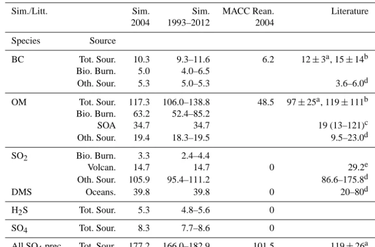
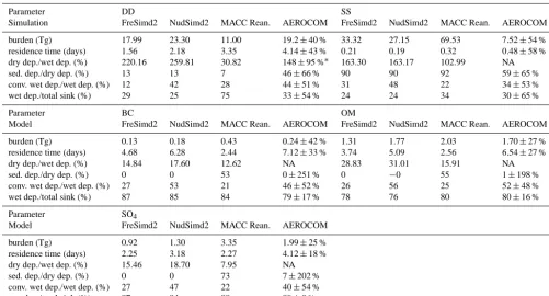
The resulting yearly totals emitted appear in Table 2, dis-tinguishing the biomass burning, the natural and the other sources. Total emissions are higher in our simulations than in the MACC Reanalysis (see further details on the MACC Reanalysis emissions in Sect. 3.2.1) for all aerosols, but all our totals are within the ranges provided in the literature (see also Table 2). A significant part of the intra- and interannual variabilities comes from the biomass burning emissions (not shown), with the biomass burning sources representing 49, 54, and 3 % of the total sources for BC, OM, and sulfate pre-cursor emissions, respectively, in 2004, which is the refer-ence year chosen for four of our simulations (see Sect. 3.1).
3 Simulations performed and evaluation data used 3.1 Simulations
M. Michou et al.: A prognostic aerosol scheme (v1) in CNRM-CM6 507
Table 2. Prescribed emission totals, including those used for the 2004 simulations, the 2003–2012 transient simulations, the MACC
Reanal-ysis, and totals reported in the literature.
Sim./Litt. Sim. Sim. MACC Rean. Literature
2004 1993–2012 2004
Species Source
BC Tot. Sour. 10.3 9.3–11.6 6.2 12±3a, 15±14b
Bio. Burn. 5.0 4.0–6.5
Oth. Sour. 5.3 5.0–5.3 3.6–6.0d
OM Tot. Sour. 117.3 106.0–138.8 48.5 97±25a, 119±111b
Bio. Burn. 63.2 52.4–85.2
SOA 34.7 34.7 19 (13–121)c
Oth. Sour. 19.4 18.3–19.5 9.5–23.0d
SO2 Bio. Burn. 3.3 2.4–4.4
Volcan. 14.7 14.7 0 29.2e
Oth. Sour. 105.9 95.4–111.2 86.6–175.8d
DMS Oceans. 39.8 39.8 0 20–80d
H2S Tot. Sour. 5.3 4.8–5.6 0
SO4 Tot. Sour. 8.3 7.7–8.6 0
All SO4prec. Tot. Sour. 177.2 166.0–182.9 101.5 119±26a
aAeroCom mean±σ(intermodel), Textor et al. (2006) Table 10.bmean±σ(intermodel), Huneeus et al. (2012) Table 5. cTsigaridis et al. (2014) mean and range from models. BC, OM and SOA (Tg yr−1),dBoucher et al. (2013) Table 7.1 range. eDentener et al. (2006). All sulfur species (Tg(SO
2) yr−1).
the satellite and AERONET data used in our evaluation (see Sect. 3.2). NudSimd2_Trans has been nudged towards the ERA-Interim Reanalysis of 1993–2012 as with NudSim.
Another difference between the free-running and the nudged ARPEGE-Climat simulations, apart from their spe-cific meteorology, is that release of aerosols in the case of stratiform precipitation re-evaporation is not applied to the free-running simulations. Such a release led to a limited num-ber of abnormally high AODs, which was sufficient to per-turb local AODs during a couple of weeks. This issue is not caused by the wet deposition formulation itself but appears to be linked to the characteristics of specific meteorological conditions along the vertical axis, which we do not encounter in the nudged simulations.
3.2 Evaluation data
3.2.1 The MACC Reanalysis data
The MACC Reanalysis, as part as the MACC FP-7 project is a 10-year long reanalysis of chemically reactive gases and aerosols using a global model and a data assimilation sys-tem based on the ECMWF IFS (see Inness et al., 2013). Its aerosol scheme is that described in Morcrette et al. (2009), so it is similar to the scheme evaluated here and its aerosol as-similation system uses MODIS AOD (Benedetti et al., 2009). Anthropogenic aerosol emissions are described in Granier et al. (2011), while the biomass burning emissions take
advan-tage of the GFAS of MACC that rests upon daily fire radiative power information from the MODIS instruments (Kaiser et al., 2012; Inness et al., 2013). The MACC Reanalysis used, as we did, the SOA climatology of Dentener et al. (2006), but did not consider any sulfur emissions from volcanoes or oceans, and no direct sulfate emissions.
The MACC Reanalysis was performed onto 60 vertical hy-brid sigma-pressure levels, with a model top at 0.1 hPa, and a T255 spectral truncation corresponding to a reduced N128 Gaussian grid with a horizontal resolution of approximately 80 km (0.7◦). Analyses of the characteristics of the simulated aerosols during this 10-year MACC Reanalysis appear in var-ious papers including those of Bellouin et al. (2013), Melas et al. (2013), Nabat et al. (2013), and Cesnulyte et al. (2014).
3.2.2 Satellite and ground-based data
prod-508 M. Michou et al.: A prognostic aerosol scheme (v1) in CNRM-CM6
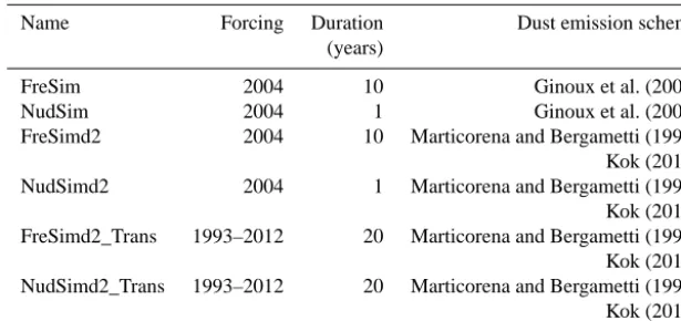
Table 3. Summary of ARPEGE-Climat simulations performed.
Name Forcing Duration Dust emission scheme
(years)
FreSim 2004 10 Ginoux et al. (2001)
NudSim 2004 1 Ginoux et al. (2001)
FreSimd2 2004 10 Marticorena and Bergametti (1995)
Kok (2011)
NudSimd2 2004 1 Marticorena and Bergametti (1995)
Kok (2011) FreSimd2_Trans 1993–2012 20 Marticorena and Bergametti (1995) Kok (2011) NudSimd2_Trans 1993–2012 20 Marticorena and Bergametti (1995) Kok (2011)
ucts that may disagree, as analysed for instance in Bréon et al. (2011) and Nabat et al. (2013), we included in our anal-ysis AOD data from the MISR (Kahn et al., 2005, 2010) on board the Terra satellite. The MISR monthly product has the same horizontal resolution as MODIS and covers the period 2001–2012.
The Cloud-Aerosol Lidar with Orthogonal Polariza-tion (CALIOP), on board the Aerosol Lidar and Infrared Pathfinder Satellite Observations (CALIPSO) satellite, is one of the very few satellite instruments providing vertical infor-mation on the aerosol distribution. We used a level-3 global monthly gridded 3-D CALIOP product that covers the years 2006–2011, already introduced at the end of the Koffi et al. (2012) paper, and under final evaluation (see Koffi in prep. and references therein). Extinction coefficients are provided at various wavelengths, under clear sky and all sky condi-tions, on a 1◦resolution grid, every 100 m from the surface up to 10 km, for all aerosols and also distinguishing the dust component. We made analysis with the 532 nm products, in all sky conditions as Koffi et al. (2012) indicates that “the cli-matology of the mean aerosol vertical extinction distribution is not significantly affected by the presence of clouds.”
AERONET is a ground-based globally distributed network of automatic sun photometer measurements of aerosol opti-cal properties every 15 min, which is a reference for AOD measurements (see Holben et al., 1998). For the present work, we used AOD monthly average quality-assured data (Level 2.0, see Holben et al., 2006) downloaded from the AERONET website (http://aeronet.gsfc.nasa.gov). Multian-nual monthly averages are available from 1993, and we re-tained in our analysis stations that included 5 years, or more, of total AOD at various spectral bands, from which we re-computed the total AOD at 550 nm when missing in the orig-inal data set, using the Ångström coefficient. AERONET AOD data have a high accuracy of <0.01 for wavelengths longer than 440 nm and<0.02 for shorter wavelengths (Hol-ben et al., 1998). We derived monthly time series and a rep-resentative station climatology from 166 AERONET stations
over the world that represent areas under the influence of var-ious dominant aerosols.
The EBAS is a database infrastructure (see http://ebas. nilu.no) operated by NILU – the Norwegian Institute for Air Research – that handles, stores and disseminates atmo-spheric composition data generated by international and na-tional frameworks like long-term monitoring programmes, including IMPROVE (United States Interagency Monitor-ing of Protected Visual Environments) and EMEP (Euro-pean Monitoring and Evaluation Programme), and research projects. For this article we downloaded and processed sur-face concentrations of SO2and sulfate. These data,
depend-ing on the network, include daily or weekly values and for the EMEP or IMPROVE networks, which provided most of the data we used, are representative of areas away from the sources. We present in this article annual means (for 2005) from all observations available.
M. Michou et al.: A prognostic aerosol scheme (v1) in CNRM-CM6 509 4 Results
4.1 Some characteristics of the ARPEGE-Climat simulations
4.1.1 Internal variability
As a preliminary step, we looked at the stability over time of the aerosol scheme. Figure 1 shows time series of global monthly mean concentrations, in the 1000–500 hPa layer, of the 12 prognostic aerosol bins over a period common to the MACC Reanalysis and our transient simulations (2003– 2012). Aside from these multi-year simulations, the diagrams include pseudo time series of the FreSim simulation that re-peated 10 times the 2004 conditions.
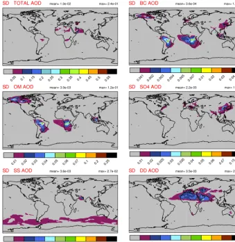
Overall, all simulations, both nudged or free-running, show no drift over time of the aerosol concentrations. Start-ing with an initial state with no prognostic aerosols, equi-librium of aerosol concentrations is reached in ARPEGE-Climat simulations within the period of a month (not shown). Figure 2 displays the interannual standard deviation (SD) of the AOD (total and five main aerosols) for JJA (June-July-August) and the FreSimd2 simulation. This SD is a represen-tation of the internal variability in ARPEGE-Climat; more-over, we present this simulation and this season, as the SD for the FreSim simulation has similar characteristics to those of the FreSimd2 simulation, and as the variability in the model for the DJF (December-January-February) season is lower for all aerosols than that for the JJA season.
SDs>0.01 are always under 20–30 % of the correspond-ing mean value, for all aerosols (not shown). Standard de-viation of the total AOD is rarely higher than 0.05, with the highest values in the biomass burning regions of cen-tral South America (SAM), southern Africa (SAF), and west of India (IND), which corresponds with larger SDs for OM and DD, respectively (see Fig. 2). Further insight into the in-ternal variability of ARPEGE-Climat total AOD is provided with figures of vertical profiles of extinction coefficients for total aerosols (see Figs. 16, 17) and for dust aerosols (see Fig. 18). A description and analysis of these figures appear in Sect. 4.2.3, but for the matter of interest in this paragraph we can say that larger SD in the SAF and SAM regions, related to the diverse spread of biomass burning aerosols (i.e., OM and BC), and in the Indian region (IND) in conjunction with variability in wet scavenging, appear to be consigned to alti-tudes below 3–4 km. In contrast, the SD of extinction coef-ficients in the central Atlantic (CAT) region, fully explained by the values and spread in dust extinction coefficients (see Fig. 18), is quite large, up to 5 km. Overall, the interannual SD of the FreSimd2 simulation is lower, for all sub-regions of the globe and for both seasons, than that of the CALIOP extinction profile product.
Overall, we can conclude from this short analysis that the internal variability of ARPEGE-Climat has little impact on
the seasonal climatology of the AODs considering both all or individual aerosols.
4.1.2 The nudged versus free-running simulations
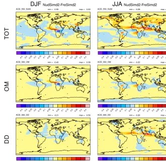
As relative differences in AOD between nudged and free-running simulations appear independent of the dust scheme (not shown), we will discuss results for the simulations with the new scheme only. Figure 1 is a first illustration of the relative behaviour of the nudged (blue lines) versus free-running (green lines) simulations. Global monthly means of aerosol concentrations from these two types of simulations appear as distinct curves except for three bins, namely the hy-drophobic OM and BC, and the sulfate precursor. In the FreS-imd2_Trans and NudSFreS-imd2_Trans simulations, these 3 bins share several common characteristics of their physical evo-lution including no wet scavenging, no sedimentation, a dry deposition independent from the meteorology, and the same prescribed emissions. The specific meteorologies of these two simulations, which govern sub-grid-scale and large-scale transport, appear then to have little impact on the global mean monthly concentrations of these three bins. For the other bins, values are in general higher for the nudged simulation, in agreement with lower wet scavenging due to lower pre-cipitation (not shown), and to the release of aerosols in the case of re-evaporation of precipitation which is suppressed in the free-running simulation (see Sect. 3.1). Total AOD in a nudged simulation (2004) without the re-evaporation pro-cess is lower by up to 20 % maximum over most of the globe (global means of −11.3 and −13.2 % in DJF and JJA, re-spectively). However, the case of sea salt, with global means lower for the NudSimd2_Trans simulation, illustrates the rel-ative importance of the various sources and sinks: with both lower dynamical emissions for DD and SS in the nudged sim-ulation (by about 8 and 14 %, respectively, see Table 5), DD concentrations are higher in the nudged simulation while SS concentrations are lower. An explanation for that, in addition to the intrinsic distributions of SS and DD, is the smaller im-portance of wet scavenging on total losses for SS than for DD with efficiencies for scavenging of, respectively, 0.2 and 0.5 (see Table 1).
510 M. Michou et al.: A prognostic aerosol scheme (v1) in CNRM-CM6Discussion
P
ap
er
|
Dis
cussion
P
ap
er
|
Discussion
P
ap
er
|
Discussion
P
ap
er
|
Fig. 1.Time series of monthly mean global bin concentrations (kg kg−1) in the lower tropo-sphere (1000 to 500 hP a layer) for the FreSimd2 Trans (green line), NudSimd2 Trans (blue line), and MACC Reanalysis (red line). In addition, dust bin concentrations are added for the FreSim simulation (black line, 2004 repeated 10 times). The 12 “bins” of the aerosol scheme are shown.
47
Figure 1. Time series of monthly mean global bin concentrations (kg kg−1) in the lower troposphere (1000–500 hPa layer) for the FreS-imd2_Trans (green line), NudSFreS-imd2_Trans (blue line), and MACC Reanalysis (red line). In addition, dust bin concentrations are added for the FreSim simulation (black line, 2004 repeated 10 times). The 12 “bins” of the aerosol scheme are shown.
Further insight into the behaviour of both types of sim-ulations is provided in Table 4, which shows global annual means of the burden, residence time and ratios of various sinks of the five aerosol types for the FreSimd2, NudSimd2, and MACC Reanalysis, while an estimation of the modelling range of these quantities is provided by Textor et al. (2006) and Huneeus et al. (2011). Burden and residence times are higher for the NudSimd2 than for the FreSimd2 simulation for all aerosol types except SS, which is coherent with the results of Fig. 1 previously analysed in this section. Values for both simulations are within the Textor et al. (2006), and Huneeus et al. (2011) mean±2σ range, except in FreSimd2 for SO4with too low burden and residence time, and in both
simulations for SS with too large burdens. However, Gry-the et al. (2014) report a spread of more than 70 Pg yr−1in the “best” SS source functions studied, which would gener-ate much higher burdens than those of Textor et al. (2006). While the dry dep./wet dep. ratios are similar or lower for the FreSimd2 simulation than for the NudSimd2 simulation, the conv. dep./wet dep. ratios are about 2–3 times smaller for FreSimd2, and the wet dep./total sink ratios a little larger for FreSimd2. Finally, the sed. dep./dry dep. ratios, not null only for the coarser SS and DD bins, are the same for both
simulations as dry deposition and sedimentation of large par-ticles are independent from meteorology. In the end, more NudSimd2 results than FreSimd2 results shown in this table are closer to the AEROCOM means. Figures computed from the MACC Reanalysis diagnostics are also presented in Ta-ble 4 but should be taken as indicative only, as an error has been identified in the wet deposition amounts (up to 50 % maximum), leading to an overestimation of the wet deposi-tion diagnostics that results, for instance, in smaller MACC Reanalysis residence times. Apart from that error, MACC Reanalysis burden amounts appear too high for SS and SO4.
4.1.3 Impact of the dust scheme
To-M. Michou et al.: A prognostic aerosol scheme (v1) in CNRM-CM6 511
Discussion
P
ap
er
|
Dis
cussion
P
ap
er
|
Discussion
P
ap
er
|
Discussion
P
ap
er
|
Fig. 2.
Mean standard deviation for JJA for the FreSimd2 simulation, as a representation of
the ARPEGE-Climat internal variability, of the total, BC, OM, sulfate, SS, and DD AODs. Color
scales are the same as in Figure 5 and 7.
48
Figure 2. Mean standard deviation for JJA for the FreSimd2 simulation, as a representation of the ARPEGE-Climat internal variability, of
the total, BC, OM, sulfate, SS, and DD AODs. Colour scales are the same as in Figs. 5 and 7.
tals in the regions may not have been consistently high (re-spectively low) within the same model, and our NudSimd2 simulation shows totals for the Middle East and Australia outside of the AEROCOM ranges, with particularly large emissions in Australia. This suggests that further adjustments of the scheme should be studied, and a simple adjustment could concern, for instance, the threshold of bare soil fraction within a grid cell required to trigger DD emissions. Such ad-justments would depend on the underlying meteorology; the impact of the lowest level and surface meteorology is clearly seen with global emissions of the NudSimd2 simulation be-ing only about 92 % of the correspondbe-ing simulation with ARPEGE-Climat meteorology (i.e., FreSimd2 simulation).
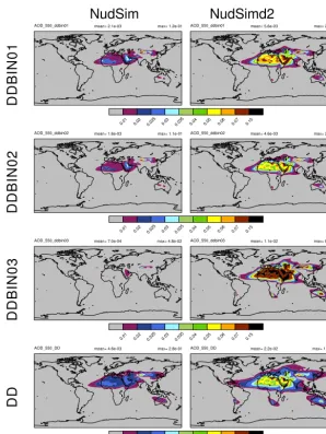
Total DD emissions are multiplied by a factor of 14 by this change of emission scheme (NudSim versus NudSimd2 simulation), knowing that factors are of 2.8, 2.9 and 20.9 for DDbin01, DDbin02 and DDbin03, respectively. These fac-tors are large but we think that the Marticorena and Berga-metti (1995) and Kok (2011) scheme is more realistic to use in the end, for the reasons detailed in Sect. 2.3.2. The cor-responding changes in AOD, for the three dust bins and the
total dust aerosol are shown in Fig. 4. The figure highlights also that the dust AOD pattern obtained with the new emis-sion scheme is much more inhomogeneous than with the old scheme (this figure) and the MACC Reanalysis (Fig. 5). This is in better agreement with the satellite MISR and Deep Blue output (Figs. 6, 7), and it reflects the soil characteristics taken into account in the new dust scheme (see Sect. 2.3.2). In the end, the mean global total DD AOD is enhanced by 4.8.
4.1.4 ARPEGE-Climat simulations versus the MACC Reanalysis
512 M. Michou et al.: A prognostic aerosol scheme (v1) in CNRM-CM6
Discussion
P
ap
er
|
Dis
cussion
P
ap
er
|
Discussion
P
ap
er
|
Discussion
P
ap
er
|
DJF
NudSimd2-FreSimd2JJA
NudSimd2-FreSimd2T
O
T
O
M
D
D
Fig. 3.
Differences in AOD between the NudSimd2 and the FreSimd2 simulations, for DJF (left
column) and JJA (right column), and for total AOD (first row), OM AOD (second row) and DD
AOD (last row).
49
Figure 3. Differences in AOD between the NudSimd2 and the FreSimd2 simulations, for DJF (left column) and JJA (right column), and for
total AOD (first row), OM AOD (second row) and DD AOD (last row).
al., 2014). However, a few deficiencies have been underlined (Melas et al., 2013), such as dust being associated with too small particles and, thus, being overly transported to regions very remote from the sources. Another deficiency is that sea salt seems to be overestimated and contributes to a high AOD bias in southern oceanic regions.
The results of the comparison between our model output and the MACC Reanalysis are the following, noting that BC comparisons between the MACC Reanalysis and our simula-tions cannot be fairly made as an unrealistic hydrophobichydrophilic frac-tion was assumed in the MACC Reanalysis (see Table 1).
Global means of tropospheric binned concentrations are shown in Fig. 1 for the MACC Reanalysis (red lines) and the NudSimd2_Trans simulation (blue lines). Concentrations of the various bins from our simulations are biased low com-pared to the MACC Reanalysis, except for the hydrophobic bins, this being possibly linked to the suppression of wet scavenging in our scheme (see Table 1), and, linked to our new dust scheme, for the two coarser dust bins. Modifica-tions of the constants of the aerosol scheme to trigger higher concentrations (see Sect. 2.3.1), in parallel with enhancement of prescribed emissions (see emission totals in Table 2),
re-sulted in these very different global monthly means. Differ-ences in sea salt concentrations are particularly striking.
Analysis of global maps of AODs (see Fig. 5) reveals that transport away from the sources is more efficient with the MACC Reanalysis meteorology than with the meteorologi-cal conditions of our nudged simulation. In the end, lower global mean values of the NudSimd2_Trans simulation in Fig. 1 are caused by lower concentrations away from the source regions. This is the case for all smaller aerosols with no or little sedimentation, and is clearly visible for instance for BC, OM and sulfate. In the case of SS, in addition to long-range transport characteristic of the MACC Reanalysis, concentrations or AODs are larger in the MACC Reanalysis even at the source regions with higher emissions (64.2 ver-sus 51.6 Pg yr−1). However, as SS in the MACC Reanalysis seems to be overestimated (see above), we chose to go along in this paper with our modelled SS distributions.
M. Michou et al.: A prognostic aerosol scheme (v1) in CNRM-CM6 513
Discussion
P
ap
er
|
Dis
cussion
P
ap
er
|
Discussion
P
ap
er
|
Discussion
P
ap
er
|
NudSim
NudSimd2
D
D
B
IN
0
1
D
D
B
IN
0
2
D
D
B
IN
0
3
D
D
Fig. 4.
Mean 2004 dust AOD for the NudSim (first column), and the NudSimd2 (second column)
simulations, for the three dust bins, from the smallest (first row) to the largest (third row), and
total DD AOD in fourth row.
50
Figure 4. Mean 2004 dust AOD for the NudSim (first column), and the NudSimd2 (second column) simulations, for the three dust bins, from
the smallest (first row) to the largest (third row), and total DD AOD (fourth row).
In summary, we demonstrated that (1) in a climatological perspective ARPEGE-Climat free-running and nudged sim-ulations show little differences and (2) the new dust scheme performs much better than the original one, we will con-tinue in the remainder of this paper with the analysis of the NudSimd2_Trans simulation only against observations.
4.2 ARPEGE-Climat simulations versus satellite and ground-based data
4.2.1 Total AOD
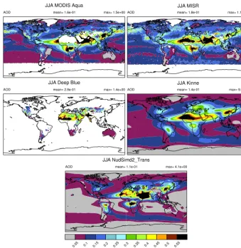
Figures of total AOD (Fig. 6 and following) show DJF and JJA means over 2003–2012 of the three satellite data sets, i.e., MODIS Aqua standard and Deep Blue products and MISR, of our NudSimd2_Trans simulation, and of the Kinne et al. (2013) climatology representative of the year 2000. The
main spatial patterns as well as the local seasonal cycles of the total AOD in various regions of the globe, in conjunction for instance with JJA dust emissions in northern Africa or the Middle East, or biomass burning in central Africa, or sea salt production in the southern oceans, are clearly depicted by the model. However, overall, model output underestimates satel-lite observations, noting that the three satelsatel-lite data sets may greatly disagree over large areas.
514 M. Michou et al.: A prognostic aerosol scheme (v1) in CNRM-CM6
Table 4. Burden, residence time and ratios for various sinks from the FreSimd2 simulation (mean over the 10 repeated 2004 years), the
NudSimd2 simulation (year 2004), the MACC Reanalysis (2003–2012 mean), and the AEROCOM models reported in Textor et al. (2006) (mean±σ, see Table 10).
Parameter DD SS
Simulation FreSimd2 NudSimd2 MACC Rean. AEROCOM FreSimd2 NudSimd2 MACC Rean. AEROCOM burden (Tg) 17.99 23.30 11.00 19.2±40 % 33.32 27.15 69.53 7.52±54 % residence time (days) 1.56 2.18 3.35 4.14±43 % 0.21 0.19 0.32 0.48±58 % dry dep./wet dep. (%) 220.16 259.81 30.82 148±95 %∗ 163.30 163.17 102.99 NA sed. dep./dry dep. (%) 13 13 7 46±66 % 90 90 92 59±65 % conv. wet dep./wet dep. (%) 12 42 28 44±51 % 31 48 22 34±53 % wet dep./total sink (%) 29 25 75 33±54 % 24 24 34 30±65 %
Parameter BC OM
Model FreSimd2 NudSimd2 MACC Rean. AEROCOM FreSimd2 NudSimd2 MACC Rean. AEROCOM burden (Tg) 0.13 0.18 0.43 0.24±42 % 1.31 1.77 2.03 1.70±27 % residence time (days) 4.68 6.28 2.44 7.12±33 % 3.74 5.09 2.56 6.54±27 % dry dep./wet dep. (%) 14.84 17.60 12.62 NA 28.83 31.01 15.91 NA sed. dep./dry dep. (%) 0 0 53 0±251 % 0 −0 55 1±198 % conv. wet dep./wet dep. (%) 27 53 21 46±52 % 26 56 25 52±48 % wet dep./total sink (%) 87 85 84 79±17 % 78 76 80 80±16 % Parameter SO4
Model FreSimd2 NudSimd2 MACC Rean. AEROCOM burden (Tg) 0.92 1.30 3.35 1.99±25 % residence time (days) 2.25 3.18 2.27 4.12±18 % dry dep./wet dep. (%) 15.46 18.70 7.95 NA sed. dep./dry dep. (%) 0 0 73 7±202 % conv. wet dep./wet dep. (%) 27 47 22 40±54 % wet dep./total sink (%) 87 84 88 89±8 %
∗Huneeus et al. (2012) values. DD, SS, BC, OM and SO
4aerosols are presented.
Table 5. Upper part of the table: dust emissions (Tg yr−1) over regions defined in Huneeus et al. (2011), for the FreSim and FreSimd2 simulations, the NudSim and NudSimd2 simulations (year 2004), the MACC Reanalysis (2003–2012 mean), and results from 15 AEROCOM models analysed in Huneeus et al. (2011), median, min, and max values. In italic font, totals lower than the AEROCOM min, in bold font, totals higher than the AEROCOM max. Lower part of the table: global sea salt emissions (Pg yr−1), with a range from Grythe et al. (2014).
Dust
Tg yr−1 FreSim/FreSimd2 NudSim/NudSimd2 MACC Rean. AEROCOM Median
Region (min–max)
Global 330/3916 256/3597 313 1123 (514:4313)
North Africa 98/1226 66/1034 88 792 (204:2888)
Middle East 59/621 51/572 37 128 (26:531)
Asia 75/455 61/405 75 137 (27:873)
South America 0/47 0/48 2 10 (0:186)
South Africa 5/72 3/51 12 12 (3:57)
Australia 31/257 20/174 47 31 (9:90)
North America 1/11 1/13 16 2 (2:286)
Sea Salt
Pg yr−1 FreSim NudSim MACC Rean. Range Grythe et al. (2014)
Global 59.9 51.6 64.2 1.8 to 605.0
biomass burning in tropical regions, while dust appears over-estimated over the Arabian Sea. Over continents in JJA, at mid to northern latitudes, the bias appears quite patchy, with both positive and negative values.
M. Michou et al.: A prognostic aerosol scheme (v1) in CNRM-CM6 515
Discussion
P
ap
er
|
Dis
cussion
P
ap
er
|
Discussion
P
ap
er
|
Discussion
P
ap
er
|
MACC Rean.
MODEL
B
C
O
M
S
O
4S
S
D
D
Fig. 5.
Mean AOD (2003-2012) for the MACC Reanalysis (first column), and the
NudSimd2 Trans simulation (second column), for BC, OM, sulfate, SS and DD.
51
Figure 5. Mean AOD (2003–2012) for the MACC Reanalysis (first column), and the NudSimd2_Trans simulation (second column), for BC,
OM, sulfate, SS and DD.
Kinne et al. (2013) climatology. As a consequence, relative biases between model output and the other two satellite data sets, i.e., the MODIS Aqua and the Deep Blue products, yielded different results; see Figs. 8 and 9. This is particu-larly the case over South America and Australia with large areas of observed low AODs (lower than 0.1). Over mid- to high-latitude oceans, the bias between Kinne et al. (2013) and our simulation is lower (around 10–50 %) than the bias between MISR and our simulation (around 30–70 %).
4.2.2 Fractional AOD
516 M. Michou et al.: A prognostic aerosol scheme (v1) in CNRM-CM6Discussion
P
ap
er
|
Dis
cussion
P
ap
er
|
Discussion
P
ap
er
|
Discussion
P
ap
er
|
Fig. 6. Mean DJF 2003-2012 total AOD for the MODIS Aqua, MISR, MODIS Deep-Blue and Kinne et al. (2013) data sets (from the top in the direction of reading), and from the NudSimd2 Trans simulation (third row).
52
Figure 6. Mean DJF 2003–2012 total AOD for the MODIS Aqua, MISR, MODIS Deep-Blue and Kinne et al. (2013) data sets (from the top
in the direction of reading), and from the NudSimd2_Trans simulation (third row).
which complements the coarse mode, the anthropogenic sul-fate aerosols (in our case sulsul-fate from all sources, including natural sources such as oceans or volcanoes), and the natu-ral aerosols (in our case DD and SS aerosols). This grouping may not appear fully satisfactory, the anthropogenic sulfate aerosols would for instance have been best identified run-ning a supplementary simulation with pre-industrial condi-tions (Schulz et al., 2006; Myhre et al., 2013) or applying more complex grouping methodologies such as in Bellouin et al. (2013), and Sessions et al. (2015), but the comparison detailed below is intended as a first estimation of our model output.
Higher coarse-mode AODs are associated with dust (e.g., northern Africa) and sea salt (e.g., Southern Ocean), whereas higher fine-mode AOD contributions are registered over re-gions of urban pollution and rere-gions affected by biomass burning. As these two modes complement each other, a model underestimation of the former goes with a model over-estimation of the latter and vice versa. In general, the model overestimates the fine-mode fraction over continents and at high latitudes (by 20 % or more), except for the very north-ern part of Africa, the Mongolian desert region, and the
trop-ical Pacific Ocean. The comparison is better for oceans, with large areas within 20 % of the Kinne et al. (2013) climatol-ogy, the northern tropical Atlantic excepted.
The sulfate fractions of the total AODs of Kinne et al. (2013) and the NudSimd2_Trans simulation show similari-ties in their hemispheric repartition, with fractions lower than 0.3 in most of the Southern Hemisphere. Over Europe and the United States, however, our fractions appear too high (by 20–80 %). This is also the case over regions in pristine air af-fected only by volcanoes, such as the Hawaiian Islands or the Antarctic continent (Mount Erebus volcano), which is coher-ent with the Kinne et al. (2013) sulfate fraction consisting of anthropogenic sulfate only.
Finally, the fraction of natural aerosols is correctly simu-lated over the oceans and dust-producing regions. Over the rest of the continents, we underestimate this fraction (by 60– 90 %) as we could not include in this fraction the contribution from second organic aerosols, which is not a simulation out-put.
M. Michou et al.: A prognostic aerosol scheme (v1) in CNRM-CM6 Discussion 517
P
ap
er
|
Dis
cussion
P
ap
er
|
Discussion
P
ap
er
|
Discussion
P
ap
er
|
Fig. 7.Same as Figure 6, for JJA.
53
Figure 7. Same as Fig. 6, for JJA.
Discussion
P
ap
er
|
Dis
cussion
P
ap
er
|
Discussion
P
ap
er
|
Discussion
P
ap
er
Fig. 8.DJF total AOD mean relative differences (2003-2012): 100(NudSimd2 Trans-x)/x, with
x=MISR first row/column, and x=Modis Aqua or x=MODIS Deep Blue or x=Kinne et al.(2013) in the direction of reading.
6
Figure 8. DJF total AOD mean relative differences (2003–2012): 100(NudSimd2_Trans−x)/x, withx=MISR first row/column,x=Modis Aqua,x=MODIS Deep Blue, andx=Kinne et al. (2013) in the direction of reading.
518 M. Michou et al.: A prognostic aerosol scheme (v1) in CNRM-CM6
Discussion
P
ap
er
|
Dis
cussion
P
ap
er
|
Discussion
P
ap
er
|
Discussion
P
ap
er
|
Fig. 9.Same as Figure 8, for JJA.
55
Figure 9. Same as Fig. 8, for JJA.
Discussion
P
ap
er
|
Dis
cussion
P
ap
er
|
Discussion
P
ap
er
|
Discussion
P
ap
er
|
Kinne Model 100*(Mod.-Kin.)/Kin.
F
R
A
C
.
F
IN
E
F
R
A
C
.
S
U
L
F
A
T
E
F
R
A
C
.
N
A
T
U
R
A
L
Fig. 10. Mean annual fractional AOD from theKinne et al.(2013) climatology (first colunm), NudSimd2 Trans simulation (1996-2005) (second column) and relative difference between the two data sets: fraction of fine mode (first row), of sulfate (sulfate row), and of natural aerosols (thirs row) (see text for details).
56
Figure 10. Mean annual fractional AOD from the Kinne et al. (2013) climatology (first column), NudSimd2_Trans simulation (1996–2005)
(second column) and relative difference between the two data sets: fractions of fine-mode (first row), of sulfate (second row), and of natural aerosols (third row) (see text for details).
on the modelling of sulfate. Correlation between model outputs and observations is better for the European sites (red dots) than for the US sites (black dots), noting that in all cases it is lower than 0.4. While for sulfate the means of observations and model outputs are very close (∼0.7), for SO2 the mean model value is twice that of the mean
observed value, some of this overestimation being related to our sulfate precursor including H2S and DMS in addition to
SO2.
M. Michou et al.: A prognostic aerosol scheme (v1) in CNRM-CM6 519
Discussion
P
ap
er
|
Dis
cussion
P
ap
er
|
Discussion
P
ap
er
|
Discussion
P
ap
er
|
Fig. 11. Scatter plot of observations (EBAS database, see text) and corresponding NudSimd2 Trans output: mean annual surface concentrations (2005) of (left) observed SO2(µg(S) m−3) and modelled sulfate precursor, (right) sulfate (µg(S) m−3). Red dots are mostly for European sites, while black dots are for US sites. Means of all observations, all model output and correlation coefficients (R) are shown.
57
Figure 11. Scatter plot of observations (EBAS database, see text)
and corresponding NudSimd2_Trans output: mean annual surface concentrations (2005) of (left) observed SO2(µg(S) m−3) and mod-elled sulfate precursor, and (right) sulfate (µg(S) m−3). Red dots are mostly for European sites, while black dots are for US sites. Means of all observations, all model output and correlation coefficients (R) are shown.
the monthly climatological AOD at 550 nm, computed over all years of data available at each given AERONET station. The NudSimd2_Trans binned AODs, at the locations of the AERONET sites, appear in the same figure grouped into SS, DD, OM, BC and SO4AODs, in addition to the AERONET
total AOD, and allow then for an evaluation of the various fractions of the total AOD. These AERONET sites cover var-ious parts of the globe (see Fig. 12 for their locations) and are categorised in three groups depending on the typically dominating aerosol type: urban/anthropogenic for the Ispra, Kanpur, La Jolla, Thessaloniki and Xianghe sites; biomass burning for the Alta Floresta and Mongu sites; and dust for the Cabo Verde, El Arenosillo, Ilorin, La Parguera and Solar Village sites.
The annual cycle of the total AOD is generally well repre-sented by the model, with either a unique narrow peak during the year, such as at the biomass burning site of Alta Floresta in South America, or a peak over several months such as at the dust site of Solar Village in Saudi Arabia, or two peaks as in Kanpur, northern India, which coincide with the pre-and post-monsoon seasons. The model is also able to capture the range of AODs covered by this selection of areas, going from total AODs lower than 0.2 all year round at La Jolla or El Arenosillo, to medium AODs (around 0.5 in Cabo Verde), and to large AODs around 1 (Alta Floresta). Another char-acteristic of the model is that, in almost all cases, it shows a low bias.
The low bias is particularly important for the Ispra site (mean yearly bias – MB – of 0.11) with sulfate as the domi-nant aerosol all year round in observations (Cesnulyte et al., 2014), as it is also the case in the model output. This under-estimation could be questioned as the data quality score of Kinne et al. (2013) is moderate only for this ISPRA site, the remaining of the Cesnulyte et al. (2014) sites having an ex-cellent quality score. Furthermore, the two nearby sites at the
Figure 12. Location of the AERONET stations presented in Fig. 13
with names in black and in Fig. 15 with names in red for poor per-formance and in green for good perper-formance.
regional scale, Thessaloniki and El Arenosillo, show much better agreement between the model and the observed clima-tologies, noting however that the dust and sulfate contribu-tions differ for all three sites; for instance, El Arenosillo can be affected by dust storms from northern Africa.
The two Asian sites of Kanpur and Xianghe are also af-fected by high pollution, and large observed AODs (larger than 0.4) prevailing all year round are underestimated in our simulation by a factor of ∼1.8. The underestimation is even larger at Ilorin (MB=0.38), located in sub-Saharan Africa, particularly in the dry season months from Novem-ber to April. This site is obviously under the influence of dust storms; however, Cesnulyte et al. (2014) indicate that fine aerosol from biomass burning make a significant contri-bution during this dry season, which is a contricontri-bution that we seem to be underestimating.
At the two shore/ocean sites of La Jolla (Pacific shore) and of La Parguera (Caribbean Islands), with relatively clean air all year round (total AOD lower than 0.25), the model underestimation appears related to an underestimation of the dust AOD, with dust transported from the nearby Mojave or further away Sahara, respectively (Cesnulyte et al., 2014).
Nevertheless, agreement between model and observations is particularly good at the two biomass sites: Alta Floresta in South America and of Mongu in southern Africa, which is more of a savannah region. This is also the case at the two dust sites: Solar Village in the heart of the Arabian Peninsula, with a small negative MB of−0.07, and Cabo Verde located∼730 km of the Senegal coast. The dust trans-port seems well represented here, although slightly underes-timated (MB=0.09).
520 M. Michou et al.: A prognostic aerosol scheme (v1) in CNRM-CM6
Figure 13. Monthly climatology of AOD, computed from all years of available data, for the AERONET stations of Cesnulyte et al. (2014).
Total observed AOD, and SO4, BC, OM, DD and SS AODs from the NudSimd2 simulation are displayed.
as ocean, mountain, polar, biomass, coastal, dust, polluted, and land; see Kinne et al. (2013). The most common loca-tions are land (46 staloca-tions), coastal (26), and polluted (25). For graphical purposes, negative correlation coefficients have been set to 0, and normalised standard deviations higher than 1.75 have been set to 1.75. Overall, the model performs rather satisfactorily with regards to the time correlation between ob-served and modelled values: the majority of series has corre-lation coefficients higher than 0.5 (118 stations), this coeffi-cient being higher than 0.7 for 64 stations. With regards to the variability of the series, the diagram reports on the ratio
between model and observed standard deviations, and indi-cates that this ratio is below 0.5 for 29 stations, while it lies between 0.5 and 1.5 for 122 stations.
M. Michou et al.: A prognostic aerosol scheme (v1) in CNRM-CM6 521
Discussion
P
ap
er
|
Dis
cussion
P
ap
er
|
Discussion
P
ap
er
|
Discussion
P
ap
er
|
Fig. 14.
Taylor diagram (
Taylor
, 2001) for the AOD monthly time series of 166 AERONET
sta-tions and ouputs from the NudSimd2 Trans simulation (see text for details). The qualification
of the stations is that of
Kinne et al.
(2013) indicating the site dominant aerosol category (O,
ocean; M, mountain; A, polar; B, biomass; C, coastal; D, dust; P, polluted, L, land), and X, no
qualification.
60
Figure 14. Taylor diagram (Taylor, 2001) for the AOD monthly
time series of 166 AERONET stations and outputs from the NudSimd2_Trans simulation (see text for details). The qualifica-tion of the staqualifica-tions is that of Kinne et al. (2013) indicating the site’s dominant aerosol category (O, ocean; M, mountain; A, polar; B, biomass; C, coastal; D, dust; P, polluted, L, land), and X, no quali-fication.
these stations have a data quality score of 3 (excellent), and a representativeness score varying between 900 and 100 km. This selection addresses several dominant aerosol types and locations in the world (see Fig. 12).
The Tahiti graph illustrates here again the poor perfor-mance of the model over oceans: as in the La Parguera case (see above in this section), the model is all the time too low and misses higher levels of AOD. The Dhadnah and Grande SONDA cases (qualified as performing well) confirm the good climatologies seen for the relatively nearby stations of Solar Village and Alta Floresta by Cesnulyte et al. (2014). In these regions the model appears to perform well over large areas. Similarly, the behaviour of the model is coherent at the Taihu station in China and at the corresponding station of Xianghe (Cesnulyte et al., 2014), with the same underes-timation of the observations.
In contrast, while the three stations of IMS-METU-ERDEMLI, Toulon, and Belsk perform poorly, either be-cause of a poor CC or a poor rVar, the Villefranche station located in the same region of the world performs well. This underlines the challenge of modelling aerosols in that Euro-Mediterranean region (Nabat et al., 2013, 2014b). The case of Arica, with a MB of 0.22 and an rVar of 0.30 requires further investigation regarding specific conditions, represen-tativity, and quality of the site, which goes beyond the scope of this paper. Finally, to finish on this comparison, which is particularly difficult for a climate model, the cases of Halifax
and Lake Argyle, with very different component distributions to the total AOD but with similarly good results, are encour-aging.
4.2.3 Evaluation of vertical distributions
Figures 16 and 17 display mean vertical profiles of total ex-tinction coefficients (km−1) for DJF and JJA, respectively, averaged for individual years. These years cover the 2006– 2011 period for the CALIOP instrument, and are representa-tive of the 2004 year for the FreSimd2 simulation (previously mentioned in Sect. 4.1.1) and the NudSimd2 simulation. We diagnosed vertical information to compare with the CALIOP data from these two simulations only. Profiles are presented for the 12 regions displayed in Koffi et al. (2012), represen-tative of regions with a dominance of marine aerosols (NAT, CAT and NWP regions), of industrial aerosols (EUS, WEU, IND and ECN regions), of dust aerosols (NAF and WCN regions), and of biomass burning aerosols (SAM, CAF, and SAF regions). In addition to these figures, Fig. 18 shows ver-tical profiles of dust extinction coefficients (km−1), for the same simulations/observations as Figs. 16 and 17, for DJF and JJA, and for the six Koffi et al. (2012) regions with a significant contribution of dust aerosols.
522 M. Michou et al.: A prognostic aerosol scheme (v1) in CNRM-CM6
Discussion
P
ap
er
|
Dis
cussion
P
ap
er
|
Discussion
P
ap
er
|
Discussion
P
ap
er
|
Fig. 15.
Times series of monthly AODs, for a selection of poorly performing AERONET
sta-tions, first six images, and of well performing AERONET stasta-tions, last six images, according
to the Taylor diagram of Figure 14. The same AODs as in Figure 13 are shown. rVar: ratio of
observed versus modelled standard deviations, CC: correlation coefficient between observed
and modelled time series, and MB: mean bias.
61
Figure 15. Times series of monthly AODs for a selection of poorly performing AERONET stations, first six images, and of well-performing
AERONET stations, last six images, according to the Taylor diagram of Fig. 14. The same AODs as in Fig. 13 are shown. rVAR: ratio of observed versus modelled standard deviations, CC: correlation coefficient between observed and modelled time series, and MB: mean bias.
The seasonality in the vertical profiles of NAF and CAT ap-pears clearly in the model and in the observations, with dust at higher levels due to transport from easterly winds reaching up to 6 km, and advection of the Saharan dust to the Atlantic between 2 and 5 km (see Fig. 17). Lastly, for the Indian in-dustrial region (IND) the NudSimd2 simulation generates an S curve shape in JJA that appears quite unique and could be related to an overly large wet deposition sink.
M. Michou et al.: A prognostic aerosol scheme (v1) in CNRM-CM6 523
Figure 16. Mean DJF vertical profiles of extinction coefficients (km−1) for total aerosols for the FreSimd2 simulation (orange lines) for 2004 (repeated 10 times), the NudSimd2 simulation (red line), and for individual years of the CALIOP 3-D product (black lines), over 12 regions of the globe, as in Koffi et al. (2012) (see in top right corners of individual figures). (X) indicates regions also presented in Fig. 18.
for NWP (north-western Pacific), with very low extinction coefficients and, for instance, for CAF in DJF or for CAT in the 2–4 km layer in JJA. Agreement is poor for other re-gions/layer depths such as the DJF CAT 0–2 km range.
5 Conclusions
We have introduced a prognostic aerosol scheme (v1) within the atmospheric component ARPEGE-Climat of the CNRM-CM6 climate model (Voldoire et al., 2012). Until now, aerosols were prescribed to the model as monthly AODs.
This scheme is based on the GEMS/MACC aerosol mod-ule included in the ARPEGE/IFS ECMWF operational fore-cast model since 2005 (Morcrette et al., 2009), which de-scribes the physical evolution of the five main types of aerosols: BC, OM, DD, SS and sulfate. A total of 12
trac-ers are distinguished in the parameterisations of the physical evolution of the aerosols, which include dry and wet deposi-tion, sedimentadeposi-tion, hygroscopic growth, conversion for sul-fate precursors into sulsul-fate, and dynamical emissions of dust and sea salt. Large-scale (advection) and sub-grid-scale (i.e., diffusion and convection) transport of these additional prog-nostic fields of the atmospheric model are also considered.