https://doi.org/10.5194/gmd-11-1321-2018 © Author(s) 2018. This work is distributed under the Creative Commons Attribution 4.0 License.
The regional climate model REMO (v2015) coupled with the 1-D
freshwater lake model FLake (v1): Fenno-Scandinavian climate
and lakes
Joni-Pekka Pietikäinen1, Tiina Markkanen1, Kevin Sieck2, Daniela Jacob2, Johanna Korhonen3, Petri Räisänen1, Yao Gao1, Jaakko Ahola1, Hannele Korhonen1, Ari Laaksonen1, and Jussi Kaurola1
1Finnish Meteorological Institute, P.O. Box 503, 00101 Helsinki, Finland
2Climate Service Center Germany, Chilehaus Eingang B, Fischertwiete 1, 20095 Hamburg, Germany 3Finnish Environment Institute SYKE, P.O. Box 140, 00251 Helsinki, Finland
Correspondence:Joni-Pekka Pietikäinen (joni-pekka.pietikainen@fmi.fi) Received: 5 October 2017 – Discussion started: 10 November 2017
Revised: 2 February 2018 – Accepted: 13 February 2018 – Published: 11 April 2018
Abstract. The regional climate model REMO was coupled with the FLake lake model to include an interactive treatment of lakes. Using this new version, the Fenno-Scandinavian cli-mate and lake characteristics were studied in a set of 35-year hindcast simulations. Additionally, sensitivity tests related to the parameterization of snow albedo were conducted. Our re-sults show that overall the new model version improves the representation of the Fenno-Scandinavian climate in terms of 2 m temperature and precipitation, but the downside is that an existing wintertime cold bias in the model is enhanced. The lake surface water temperature, ice depth and ice sea-son length were analyzed in detail for 10 Finnish, 4 Swedish and 2 Russian lakes and 1 Estonian lake. The results show that the model can reproduce these characteristics with rea-sonably high accuracy. The cold bias during winter causes overestimation of ice layer thickness, for example, at several of the studied lakes, but overall the values from the model are realistic and represent the lake physics well in a long-term simulation. We also analyzed the snow depth on ice from 10 Finnish lakes and vertical temperature profiles from 5 Finnish lakes and the model results are realistic.
1 Introduction
The interactions between the atmosphere and the underlying surface are among the most important factors in climate and numerical weather prediction (NWP) modeling (Mironov, 2008; Samuelsson et al., 2010). Land and sea surfaces are dominant globally, but regionally, lake surfaces can play a significant role. Locations like Northern Europe, Asia and North America have rather high lake area densities, and the interactions between the atmosphere and lake surface can be a major driver in regional and local climate. Thus, in order to make reliable climate simulations, models should include lake modules that have reasonable complexity to simulate in-teractions between the atmosphere and lakes (Kirillin et al., 2012).
Ex-periment for the European domain) RCMs have artificial heat sources during winter. These can be directly linked to the large fractional area of lakes, whose prescribed surface tem-peratures violate surface–atmosphere interactions. Some of the models still use a simple approach in which the lake temperatures and ice conditions are linked to the closest sea point. In reality, Fenno-Scandinavian lakes usually freeze be-fore the nearest sea area because the lakes are more shallow and consist of fresh water (Kirillin et al., 2012). This means that with the nearest sea point approach, lakes continue to emit heat and moisture to the surrounding atmosphere for far too long during early winter, thus causing artificial heat and moisture fluxes to the atmosphere.
To overcome the deficiencies in lake representation, lake models have been implemented in some RCMs (e.g., Mar-tynov et al., 2010; Samuelsson et al., 2010; Gula and Peltier, 2012; Mironov et al., 2012; Bennington et al., 2014) and NWP models (e.g., Mironov et al., 2010; Yang et al., 2013). In most cases these models resolve the vertical profiles of lake variables in 1-D without any direct horizontal influence. This approach is widely used because it is computationally efficient and has been shown to reproduce realistic lake- and climate-related variables (Kourzeneva et al., 2012; Stepa-nenko et al., 2013; Mallard et al., 2014). There are also 2-D and 3-D lake models (e.g., León et al., 2007), but these mod-els are usually much more computationally demanding than 1-D models. Furthermore, 3-D lake models require a higher-resolution computational grid (∼2 km) and lake-specific in-flow and outin-flow information (Martynov et al., 2010). In principle, a high-resolution 3-D lake model could be coupled with an RCM of lower resolution by various downscaling ap-proaches, but this would further increase the computational costs.
One widely used 1-D freshwater lake model is FLake (Mironov, 2008), which has been coupled into several cli-mate and weather models (Stepanenko et al., 2013). For ex-ample, Mironov et al. (2010) introduced FLake into the nu-merical weather prediction model COSMO and showed that the coupling improved the prediction of lake surface temper-atures, the freeze-up of lakes and the ice breakup across Eu-rope. The COSMO–FLake system eliminated the significant overestimation of the lake surface temperatures during win-ter. Samuelsson et al. (2010) showed that the implementation of FLake to the Rossby Centre regional climate model RCA reduces known biases by increasing the 2 m temperature over Europe by up to 1◦C and the precipitation by 20–40 % when compared to a simulation without lakes. Martynov et al. (2012) simulated North American climate with the Canadian Regional Climate Model (CRCM) using two different lake models: FLake and Hostetler (Hostetler and Bartlein, 1990). The authors showed that FLake performed very well over their domain, giving better results than the Hostetler model, while the large and deep lakes caused some problems for both models. Finally, Mallard et al. (2014) showed that in the Weather Research and Forecasting (WRF) model, FLake
significantly improved the timing and extent of ice coverage and reduced errors in lake temperatures.
In this study, FLake has been interactively coupled with the regional climate model REMO. With the new model ver-sion called REMO–FLake, we have simulated over 35 years of the Fenno-Scandinavian climate and compared the results against the default model version and measurement data. Moreover, the lake-related variables (e.g., surface tempera-ture, ice thickness and snow depth on ice) have been com-pared to observations for 10 Finnish, 4 Swedish and 2 Rus-sian lakes and 1 Estonian lake. Additionally, some analy-sis has been made for vertical temperature profiles in five Finnish lakes.
The article is structured as follows: first, REMO, FLake and the implementation structure are described in Sect. 2; in Sects. 3 and 4 a detailed analysis of the results is given; finally, in Sect. 5, the main conclusions are discussed.
2 Methods 2.1 REMO
In this work, the hydrostatic version of the REgional MOdel REMO (version REMO2015) has been used (Jacob and Podzun, 1997; Jacob, 2001). REMO is a three-dimensional atmosphere model developed at the Max Planck Institute for Meteorology in Hamburg, Germany and currently main-tained at the Climate Service Center Germany (GERICS) in Hamburg. The model is based on the Europa Model, the former NWP model of the German Weather Service. The prognostic variables in REMO are horizontal wind compo-nents, surface pressure, air temperature, specific humidity, cloud liquid water and ice. The physical packages origi-nate from the global circulation model ECHAM4 (Roeckner et al., 1996), although many updates have been introduced (e.g., Hagemann, 2002; Semmler et al., 2004; Pfeifer, 2006; Kotlarski, 2007; Teichmann, 2010; Pietikäinen et al., 2012; Preuschmann, 2012; Wilhelm et al., 2014).
REMO uses a leap-frog scheme with time filtering by As-selin (1972) for the temporal discretization. To allow for longer time steps a semi-implicit correction is used. The ver-tical atmospheric levels are represented in a hybrid sigma-pressure coordinate system, which follows the surface orog-raphy in the lower levels and is independent of it at higher atmospheric model levels. Horizontally, REMO has a spher-ical Arakawa C grid (Arakawa and Lamb, 1977) in which all prognostic variables except winds are calculated at the cen-ter of a grid box. The wind components are calculated at the edges of the grid boxes.
zone towards the inner model domain. At the surface, the sea surface temperature (SST) and sea ice distribution are prescribed by the lateral boundary forcing dataset. At land points, a fractional land surface scheme is used and details can be found, for example, in Kotlarski (2007) and Rechid (2009). The scheme uses a tile approach with three tiles: land, water and ice (Semmler et al., 2004). The biogeophys-ical characteristics of the land tile are described through sur-face parameters. The leaf area index, fractional green vege-tation cover and background surface albedo are prescribed with monthly values accounting for the seasonality of the vegetation characteristics (Hagemann, 2002; Rechid and Ja-cob, 2006). The background albedo has some further devel-opments in terms of pure soil and pure vegetation albedo (Rechid, 2009; Rechid et al., 2009). The soil temperature profile is resolved using five soil layers of increasing thick-nesses reaching 10 m of depth. The soil hydrology is based on a simple bucket scheme by Manabe (1969) with an im-proved accounting of the subgrid-scale heterogeneity of the field capacities within a climate model grid box (Hage-mann and Gates, 2003). The vertical diffusion fluxes due to subgrid-scale turbulence are calculated for the lowest layer (surface layer) according to Louis (1979). The 2 m temper-ature calculation is based on these fluxes (Roeckner et al., 1996). The snow parameterization is based on the ECHAM4 approach, which was later improved by Semmler (2002) for better performance in high-latitude regions. The snow layer is divided into two parts for the heat conductivity calcula-tions. A top layer (0.1 m thickness) is used for defining the surface temperature of the snowpack and serves as an inter-face to the atmosphere. The temperature in the rest of the snowpack is calculated using the top snow layer tempera-ture and the top soil layer temperatempera-ture. If the temperatempera-tures of these two snow layers reach the melting point, any further energy input is used for snowmelt. The density of the snow and the heat conductivity are parameterized as a function of the snow layer temperature (Roeckner et al., 1996; Kotlarski, 2007).
Lakes are included in REMO through the default land cover map: Global Land Cover Characteristics Database (GLCCD; Loveland et al., 2000; US Geological Survey, 2001). However, the standard land surface scheme does not have a tile for lakes and thus does not allow for their ex-plicit treatment. Instead, the model uses the nearest sea point approach for all non-seawater fractions to determine the wa-ter temperature and ice conditions. As indicated above, the nearest sea point approach can lead to a significant distor-tion of the simulated climate, which suggests that REMO would benefit from a coupling with a physical- or process-based lake model.
2.2 FLake lake model
FLake is a thermodynamic freshwater lake model, which pre-dicts the mixing conditions and vertical temperature
struc-ture of lakes on timescales from a few hours to several years (Mironov, 2008; Mironov et al., 2010). The FLake water module calculates the heat and kinetic energy budget for the upper mixed layer and the basin bottom. The model can be used for various basin depths and even though it has been in-tended for use in NWP and climate models, it can be used as a stand-alone model as well. FLake uses a bulk approach and is based on a self-similarity (assumed-shape) represen-tation of the temperature profile in the mixed layer and ther-mocline. In addition, it calculates the mixed-layer depth as well as the temperature and thickness of both ice and snow on ice. Optionally, FLake can calculate the flux between the bottom sediment and the lake bottom. In this case, the thick-ness and temperature of the thermally active upper sediment layer are calculated. A more detailed description of FLake can be found in Mironov et al. (2010), in which the authors give a detailed list of FLake parameters and more informa-tion about the numerical core.
2.3 Implementation of the FLake model
REMO surface fractions are based on the Global Land Cover Characteristics (GLCC) database (US Geological Survey, 2001). This database has a nominal 1 km spatial resolution and includes lakes as one variable. The REMO surface pre-processor, which creates the surface-related parameters in-cluding the fractions of different tiles (land, water and ice), was modified in this work to also include the lake fraction as an output variable. Thus, while the standard version of REMO lumps sea, lakes and rivers together in the water tile, here a separate tile is created for lakes and rivers. The lake depth data were taken from the detailed dataset developed by Choulga et al. (2014), which gives the mean depths of lakes in a global grid (version v3). Using a dataset with real-istic lake depths is important, as shown by Samuelsson et al. (2010). Additionally, the dataset by Choulga et al. (2014) in-cludes lake fractions, but to be consistent with the rest of the model, the GLCC lake fractions were used. In practice, this means that whenever there is a lake in the GLCC dataset, the lake depth is taken from the Choulga et al. (2014) dataset. For points for which Choulga et al. (2014) have no data, a default value is used and it can be set beforehand within the surface preprocessor. In this work, a default value of 7 m was used, which is a typical mean depth for our domain based on the data by Choulga et al. (2014).
dif-fers from the original approach, in which the fraction of sea and ice was taken from the driving data. However, as there is a resolution difference between our simulations (roughly 18 km resolution) and the driving data (ERA-Interim, ap-proximately 80 km Dee et al., 2011), the fractional ice cover values for lakes from the driving data are either 0 or mostly between 0.9 and 1. Thus, in practice, the ice fraction val-ues are close to binary already in the standard version of the model. All the tile-specific variables (e.g., specific humidity, surface temperature, surface fluxes and albedo) are now cal-culated for the lake tile by taking into account the tile state. The tile-related variables are averaged based on their fraction in a grid box and the host model uses these averaged values in the physics calculations.
The FLake model also includes a surface-flux parameteri-zation (SfcFlx). However, as REMO resolves the state of the surface and related fluxes for other tiles, for consistency we let it calculate those for the lake tile as well. Below the land surface, REMO uses a diffusion equation solver in a five-layer model with zero heat flux at the bottom (10 m). For the lake tile, this has not been used; instead, FLake’s own lake bottom sediment module has been implemented to REMO. This module calculates the heat flux at the water–bottom sed-iment interface by using the depth of the upper layer of bot-tom sediments that is penetrated by the thermal wave and the temperature at that depth. However, the bottom sediment module is important only for shallow lakes and thus we use a 5 m cutoff limit: for lakes deeper than this the bottom sed-iment module has been switched off (FLake webpage, 2018, http://www.flake.igb-berlin.de). Moreover, as FLake is not suitable for deep lakes (Mironov et al., 2010), a “false bot-tom” approach has been used. In this approach, the maximum lake depth has been set to 50 m. As a security check, the bot-tom sediment module has been switched off for lakes deeper than 50 m. This has a negligible impact on the results be-cause typically there are no significant temperature changes in such depths for freshwater lakes (Samuelsson et al., 2010). Although the 5 m cutoff limit already switches off the bottom sediment for lakes deeper than 50 m, we have kept both of these options for future testing purposes.
Even though the snow module of FLake has not been thor-oughly tested, there is some evidence that in climate simu-lations the snow module gives realistic results (D. Mironov, personal communications, 2015). We have also updated the coefficients used to calculate snow density and heat conduc-tivity as suggested by Mironov et al. (2012). These changes are needed as the original approach yielded too-low snow density and too-high snow temperature conductivity. More-over, we have implemented an alternative approach for snow heat conductivity, with an effective snow heat conductivity
kseffas proposed by Semmler et al. (2012):
kseff=ks+(ki−ks)×e−hs×c, (1) whereks is the heat conductivity of snow (0.14 W(mK)−1),
kiis the heat conductivity of lake ice (2.29 W(mK)−1),hsis
the snow depth (m) andcis an empirical constant (5 m−1). In practice, this approach increases the heat conductivity for thin snow because it is highly probable that there is also bare ice in the vicinity of thin snow due to snow redistribution by wind drift; thus, thekseffis actually a mixture of snow and ice conductivity. Due to stability issues, we start to accumulate snow over ice only when the ice layer is at least 3 cm thick. In addition, the ice albedo limits from Semmler et al. (2012) have been implemented (similar changes were also made by Yang et al., 2013). The default albedos in FLake are from 0.1 to 0.6 for ice and snow, respectively, while the ice albedo range applied in Semmler et al. (2012) is from 0.3 to 0.5. Moreover, we have changed the snow albedo limits and these changes will be shown in detail in the next section.
For all other FLake model-related variables and parame-ters the default FLake configuration has been used (Mironov, 2008; Mironov et al., 2010).
2.4 The snow albedo
Snow albedo is an important part of the energy cycle and at least in global climate models, the simulated temperature can be quite sensitive to relatively small changes in snow albedo (e.g., Räisänen et al., 2017). Lakes in the Nordic countries are usually always covered with snow during winter. The snow module of FLake does not calculate snow albedo separately and uses the same albedo for snow as for ice. Thus, as a snow albedo scheme had to be implemented for the lake tile, we have also looked into the details of the current snow albedo scheme in REMO and studied a possible alternative approach for it.
Three treatments of snow albedo αsn are considered in this work: a temperature-dependent scheme, a snow albedo scheme originating from the Biosphere–Atmosphere Trans-fer Scheme (BATS; Dickinson et al., 1993) and their combi-nation. By default, REMO employs a temperature-dependent snow albedo scheme. The shortwave radiation module for REMO separates visible and near-infrared spectral regions (VIS and NIR, respectively) for surface albedo, but in the default treatment, a broadband approach (the same albedo for the VIS and NIR regions) is used for snow albedo. The snow albedo over land is temperature dependent and obtains its maximum valueαsnmax =0.8 when the snow temperature
is below−10◦C. At higher temperaturesαsndecreases lin-early until it reaches the snow albedo minimumαsn=0.4 at the freezing point. Moreover, the forest fraction of the grid cell linearly influences the albedo maximum and min-imum values so that they reach values ofαsnmax=0.4 and
αsnmin=0.3 at a forest fraction of unity (details in Kotlarski,
2007). However, these values of forestedαsnmax andαsnmin
are slightly higher than those shown in the literature (e.g., Roesch et al., 2001, and references therein), and therefore in the present work we have reduced bothαsnmax andαsnmin to
Figure 1.Lake fraction (a, based on GLCC data) and lake depth (b, based on Choulga et al., 2014) of the calculation domain. Additionally, the surface geopotential height of Finland and the locations and names of the analyzed Finnish lakes are shown (c, based on Aalto et al., 2016).
The temperature-dependentαsntakes into account that the snow albedo is lower when snow is wet, i.e., is near the freez-ing point. However, this approach does not take into account the aging of snow, soot loading, grain size or the influence of solar zenith angle. As these play a role in αsn, in this work, we have implemented the snow albedo scheme from the Biosphere–Atmosphere Transfer Scheme (BATS; Dick-inson et al., 1993). In this scheme,αsntakes into account the aging of snow and solar zenith angle and is calculated sepa-rately for VIS and NIR. The aging of snow is based on three terms: the first represents the effect on snow grain growth due to vapor diffusion, the second represents the additional effect near and at freezing of meltwater and finally the third introduces the influence of soot and dirt through a global time-independent constant (details in Dickinson et al., 1993). The VISαsnis allowed to obtain values between 0.9 and 0.5 and the NIR αsn between 0.65 and 0.25; the highest values are employed for new snow. The forest fraction decreases these values as with the temperature-dependent broadband approach so that a fully forested grid box has a VIS snow albedo of 0.25 and a NIR albedo of 0.2.
The temperature-dependent scheme aims to describe the reversible changes in the crystal structure of snow when the temperatures approach the melting point. On the other hand, the BATS scheme describes the irreversible crusting of a snow layer and the accumulation of aerosols and other impurities in the snow through the aging factor. As these are both important in reality, we modified the source code so that one can choose either the original scheme, the new BATS scheme or a combined approach similar to that em-ployed in the JSBACH model (Raddatz et al., 2007; Brovkin et al., 2013; Reick et al., 2013). In the JSBACH approach, the
schemes are weighted and in this work we have used equal weights.
The albedo reduction due to forests only occurs over land areas. Therefore, snow albedo (and for the BATS scheme, snow aging) is calculated separately for land and lake tiles as one grid box can have snow on both tiles. The grid point snow albedo is then calculated as an area-weighted mean value of the tile albedos.
2.5 Simulations
We have made simulations for Northern Europe for the pe-riod of July 1979–March 2015. The simulations employed a warm-start method, which means that at the start of the simulation soil temperature, soil moisture and lake variables were obtained from existing simulation data. In the warm-start method, the model was run for the whole time period with default initial values (for REMO and REMO–FLake separately) and then the model state in July 2014 was used as the initial state for the actual and analyzed simulations (start-ing in July). More details about the method for the same do-main can be found in Gao et al. (2014) and Gao et al. (2015). The horizontal resolution of the simulations was 18 km×
Table 1.Simulation names with the configurations showing whether FLake is used or not, which snow albedo scheme (αsn) is used and which snow heat conductivity (ks) method is used.
Simulation FLake αsn ks(lakes)
REMO-ST No T-scheme –
REMO-FL Yes T-scheme Semmler et al. (2012) REMO-FLB Yes BATS Semmler et al. (2012) REMO-FLTB Yes T-scheme+BATS Semmler et al. (2012) REMO-FLOS Yes T-scheme FLake original
Table 2.Analyzed lakes with their mean depth, mean depths applied in REMO and the lake area information for the REMO analysis (SYKE
refers to the Finnish Environment Institute).
Lake Data source Mean depth REMO area mean REMO area REMO area (m) depth (m) longitudes latitudes
Haukivesi (Fin) SYKE 9.1 7.0 27.9↔28.9 61.9↔62.3 Inari (Fin) SYKE 14.3 13.3 27.0↔28.6 68.7↔69.2 Kallavesi (Fin) SYKE 9.7 7.0 27.4↔28.0 62.5↔63.0 Lappajärvi (Fin) SYKE 6.9 16.0 23.4↔23.9 63.1↔63.3 Näsijärvi (Fin) SYKE 13.7 7.0 23.5↔23.9 61.5↔61.9 Oulujärvi (Fin) SYKE 7.0 6.8 26.7↔28.0 64.1↔64.6 Pielinen (Fin) SYKE 10.1 9.8 29.0↔30.2 62.9↔63.6 Pyhäjärvi (Fin) SYKE 5.5 5.4 22.1↔22.4 60.9↔61.1 Päijänne (Fin) SYKE 14.2 14.5 25.1↔25.9 61.2↔62.2 Saimaa (Fin) SYKE 10.8 13.6 27.7↔28.8 61.1↔61.6 Hjälmaren (Swe) ILEC (1988–1993) 6.2 5.9 15.3↔16.3 59.1↔59.3 Mälaren (Swe) ILEC (1988–1993) 13.0 6.1 16.1↔17.1 59.2↔59.6 Vänern (Swe) ILEC (1988–1993) 27.0 22.0 12.3↔14.1 58.4↔59.4 Vättern1(Swe) ILEC (1988–1993) 41.0 29.0 14.1↔15.0 57.8↔58.8
Benson and Magnuson (2000, updated 2012)
Ladoga1(Rus) northern part ILEC (1988–1993) 51.0 62.4 29.8↔33.0 60.8↔61.8 Ladoga1(Rus) whole lake Benson and Magnuson (2000, updated 2012) 51.0 47.3 29.8↔33.0 59.9↔61.8 Onega1(Rus) ILEC (1988–1993) 30.0 25.7 34.3↔36.5 60.9↔62.9
Benson and Magnuson (2000, updated 2012)
Võrtsjärv2(Est) ILEC (1988–1993) 2.7 3.0 25.9↔26.2 58.1↔58.4
1Lake temperature from ILEC (1988–1993) and ice cover period from Benson and Magnuson (2000, updated 2012). 2Lake temperature and ice cover period from ILEC (1988–1993).
the analyzed Finnish lakes are shown. We have conducted a total of five simulations: one without FLake and four with FLake (Table 1). The simulation without FLake (REMO-ST) was conducted using the default configuration of the model. The simulations with FLake included a baseline run (REMO-FL) with the temperature-dependent snow albedo scheme, a run with the BATS snow albedo scheme (REMO-FLB) and a run with the combined temperature–BATS albedo scheme (REMO-FLTB). The fourth simulation (REMO-FLOS) was otherwise similar to REMO-FL but used the FLake origi-nal snow heat conductivity approach instead of the Semm-ler et al. (2012) approach. For all temperature-dependent snow albedo simulations (the REMO default configuration) the broadband albedo has been used, but for all simulations including the BATS scheme, the VIS and NIR separation ap-proach has been used (details in Sect. 2.4).
2.6 Lake data
The Great Saimaa Lake is the largest lake by area in Fin-land (see Table 2 and Fig. 1). However, its areal definition is not unambiguous because it is a combination of several open lake areas connected by straits. In our study, we have di-vided the Great Saimaa Lake into two parts. Lake Haukivesi is a lake between the cities of Varkaus and Savonlinna and represents the northwestern part of the Great Saimaa Lake. Another focus area in our study is the southern part where the open lake area is actually called Saimaa; i.e., in our study, the name Lake Saimaa points to the southern area of the Great Saimaa Lake.
Table 2 shows the mean lake depths and the means calcu-lated from the data by Choulga et al. (2014). It also shows the longitudinal and latitudinal boundaries that are used to define the lake area in the analysis of the model results. As can be seen, the average depths are reasonably similar be-tween the literature and model data, except at the following: Lappajärvi, for which the dataset by Choulga et al. (2014) gives a 16 m depth for the whole lake, while in reality it is closer to 7 m, at Kallavesi, Haukivesi and Näsijärvi, for which the FLake database does not have information about the depth and the default value of 7 m is used, at Mälaren, for which the overall shape of the lake is not well represented in the database and causes underestimation of the mean depth, and at Vättern for which the difference is slightly over 10 m. There is also over 10 m of difference at the northern part of Lake Ladoga, but the literature-based average depth for the whole lake has also been used for the northern part and this causes error.
Table S1 (Supplement) introduces the measurement loca-tions from the SYKE database (the localoca-tions can be seen from Fig. 1). It defines the actual locations (lake name is used if the measurement is done at the open lake or if it represents the whole lake area) and shows how many measurement sites are used in the actual analysis. If an analyzed variable has more than one source for some time period, a mean value has been used. Different sources give more information about the spatial differences of the analyzed area, which reduces the error when comparing point measurements against larger model grids. The LWTs are measured at 8:00 (local time) and all modeled LWTs are also taken from this same time of the day. Ice thickness and the snow depth on ice have been measured at different times of the day and thus the modeled daily mean value is used. The SYKE measurements for LWT, ice depth and snow on ice are done close to the lakeshore, which causes some error when compared to the lake average modeled values. This will be discussed in more detail in the following sections.
3 Climate impacts
We have compared the modeled 2 m air temperature and precipitation fields against the E-OBS version 16-gridded dataset (Haylock et al., 2008). For this comparison, the
mod-eled values were remapped to the E-OBS grid, which is slightly coarser (0.25◦) than the REMO grid. The accuracy of the E-OBS data depends on the density of the underlying measurement network and naturally this introduces some er-ror (e.g., Kotlarski et al., 2014, and references therein). We do not explicitly consider the observational uncertainties like undercatch of precipitation, but they should be kept in mind (Prein and Gobiet, 2017). Moreover, the relaxation zone, i.e., the area where the lateral forcing directly influences the re-sults, has been removed from the analysis. All shown 2 m air temperature values have been corrected with the lapse rate
γ=0.0064◦C m−1 to compensate for the effect of orogra-phy difference on temperature.
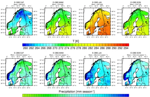
In the analysis part (Sect. 3.1) we will show only the dif-ferences between the E-OBS measurement data and model results. The absolute values from E-OBS for 2 m air temper-ature and precipitation are shown in Fig. 2. The values are year seasonal means for 2 m temperature and multi-year mean seasonal sums for precipitation.
3.1 Influence of the lake model FLake
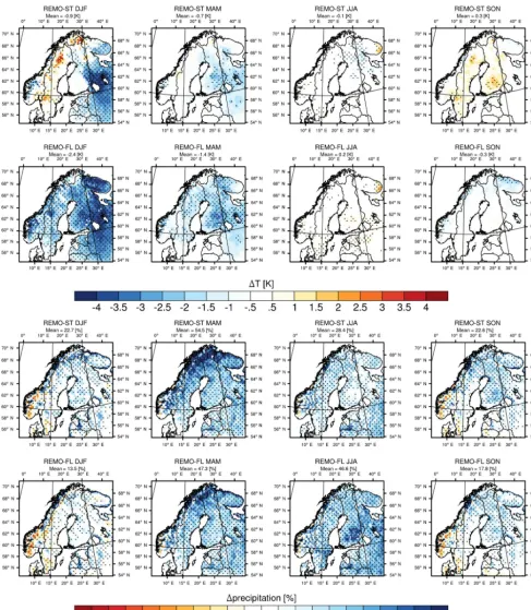
The comparison of the model results against the E-OBS 2 m air temperature and surface precipitation for the standard REMO run (REMO-ST) and for REMO–FLake (REMO-FL; details in Table 1) is shown in Fig. 3. The areas marked with dots indicate their statistical significance, withp val-ues<0.05. As the E-OBS data are based on measurements over land and the values given over lakes are an interpola-tion of these measurements, a direct comparison against the model results causes artificial biases over grid boxes with a high lake fraction. To reduce these biases, we have ex-cluded all grid points in which the lake fraction is equal or larger than 0.5. While we have no direct measurements of 2 m temperatures over lakes, we will analyze in Sect. 4.1 and 4.2 the LWTs, which are generally close to the 2 m tempera-tures over lakes when they are not frozen.
Figure 2.The reference values of 2 m temperature and precipitation from E-OBS data. The seasonally averaged results are for the time period of October 1979–March 2015.
rather than, for example, missing low-level clouds (without totally ruling out this possibility). Figure 4 shows the sur-face specific humidity and 10 m wind speed from REMO-ST and the difference between REMO-FL and REMO-REMO-ST. We can clearly see that when FLake is included, the humid-ity decreases at the surface during wintertime as the artificial moisture sources are no longer available. There are, however, some increased values over lakes Ladoga and Onega, which indicates that with FLake these lakes have more open lake pe-riods during winter than what was originally simulated based on the nearest neighbor approach. The 10 m wind speeds are also influenced by the roughness length (larger wind speeds when the roughness length is smaller). Following the hu-midity, the wintertime 10 m wind speeds are decreased in REMO-FL as the heating of the atmosphere is reduced and boundary layer stability is increased.
The spring season biases qualitatively follow the winter results in Fig. 3. REMO-ST has a smaller cold bias due to warmer temperatures over lakes (−0.7 K). REMO-FL in-creases the cold bias to−1.4 K as the lakes stay frozen longer than in REMO-ST and do not artificially pump heat to the at-mosphere (Fig. 4). The cold bias is weaker than in winter as the fraction of snow-covered surfaces decreases.
Statisti-cally, the differences in spring are significant. During sum-mer, REMO-ST has a small cold bias over the domain and REMO-FL a slight warm bias. Overall, the summer tempera-tures are captured very well in both model versions. Autumn temperatures are warm biased in REMO-ST, but much better captured by REMO-FL. The REMO-ST biases primary oc-cur near lakes and are statistically significant. This indicates that the original approach for lakes starts to heat the atmo-sphere unrealistically, while in reality lakes cool faster.
pre-Figure 3.The 2 m temperature and precipitation biases of standard REMO (REMO-ST) and REMO with the FLake module (REMO-FL) compared to E-OBS data. The seasonally averaged results are for the time period of October 1979–March 2015. Dots indicate statistically significant differences withpvalues<0.05.
cipitation biases during spring are also smaller with FLake (REMO-ST 54.5 % and REMO-FL 47.3 %) and the largest biases occur in northern Finland and the surrounding areas.
Figure 5.Monthly mean albedos for March and April from satellite data (CLARA-A2; Karlsson et al., 2017) and the corresponding bias (model–measurements) in the REMO-FL, REMO-FLB and REMO-FLTB runs. The monthly means are for the time period of 1982–2014 and only for land and lake surfaces.
The use of FLake significantly increases the precipitation bias in summer. REMO-ST has a 28.4 % bias, but REMO-FL yields a 46.6 % bias with the largest excess in precipitation in central-eastern Finland. Some overestimation can be also seen over Sweden. The increased wet bias seems to be con-nected to the fraction of lakes (Fig. 1) and is caused by the increased convective precipitation (analysis not shown here). Figure 4 shows that the surface specific humidity and 10 m wind speeds increase in these areas. With the current hori-zontal resolution (18 km×18 km), the model uses a convec-tive parameterization to calculate the convection processes based on the mass-flux scheme from Tiedtke (1989) with modifications by Nordeng (1994). With REMO-FL, the lake surfaces are warmer and thus there is more evaporation and humidity, which tends to trigger the convection. Although not shown here, we also analyzed the lake surface temperatures from the lateral boundary data, which are the standard that REMO uses. Our analysis showed that the LWTs in REMO-FL are 3–7◦C higher on average during summer than those in REMO-ST. This explains why there is more heat avail-able for triggering the convection over lakes in REMO-FL. Moreover, the increased 10 m wind speeds in REMO-FL en-hance the evaporation, which can be seen as increased near-lake surface humidity in REMO-FL. Nevertheless, we have not investigated in detail why there is excess convective pre-cipitation and only suggest possible reasons. The tion scheme works during a single time step; i.e., convec-tive clouds form and precipitate during one time step, which causes precipitation to be too localized over lakes and there is insufficient transport of moisture. Another factor might
be that the cloud cover is too small in the model because convective clouds are not radiatively active (i.e., the radia-tion scheme does not “see” convective clouds directly, but the model accounts for their transport of moisture in the large-scale cloud scheme). Naturally, the LWTs in REMO-FL could be too high, but this does not seem to be the reason, as will be seen in the later analysis.
The precipitation bias for REMO-ST during autumn (22.6 %) is higher than for REMO-FL (17.8 %). Like in win-ter, the wet bias in REMO-ST originates from lake areas: in reality, lakes cool faster than with the nearest sea point approach and this leads to excess heat and moisture near lakes in the nearest sea point approach. This can also be seen in Fig. 4 in which REMO-FL shows decreased surface hu-midity values when compared to REMO-ST. When FLake is used, temperature and moisture are more realistic, leading to smaller biases during autumn.
3.2 Snow analysis
months, our domain still has snow, and additionally we can see the impacts of the snow-melting period. Moreover, as the purpose of the comparison is to show how much the differ-ent snow albedo methods influence the results, we limit the comparison to land and lake surfaces.
Figure 5 shows the multi-year monthly measured albedos and the model bias (model–measurements) for the time pe-riod of 1982 to 2014. We compare three model versions, which are the default REMO–FLake (REMO-FL), REMO– FLake with the BATS albedo scheme (REMO-FLB) and REMO–FLake with the combined BATS and temperature albedo scheme (REMO-FLTB). Based on the albedo values, there is quite a lot of snow in our domain during March, whereas during April, the southern part of the domain is snow free. The different model versions show some differ-ences in March; for example, over the central-eastern part of the domain, REMO-FLB gives higher albedos than the simulations using the original (REMO-FL) or the combined albedo parameterization (REMO-FLTB). Overall over land, REMO-FL tends to underestimate the albedo when there is snow, but it is quite close to the measurements otherwise. The albedo over lakes in March is fairly well captured, al-though slightly overestimated with REMO-FLTB and espe-cially in REMO-FLB. In March, the lake albedos seem to be overestimated in all model versions, although with REMO-FL only slightly. The overestimation is due to the cold bias in the model, which delays the melting of snow and ice. The same features can be seen as in April: the albedo in regions with snow is slightly underestimated. We also analyzed how much the changes made to the snow albedo in forested re-gions impact the results (see Sect. 2.4), but the difference is insignificant and cannot explain the overestimation (details not shown here).
The impact of the different snow albedo parameterizations on simulated 2 m temperature and precipitation can be seen by comparing REMO-FL in Fig. 3 with REMO-FLB and REMO-FLTB in Fig. S1. Overall, the impact is small. In the experiment with the temperature-based snow albedo scheme (REMO-FL), snow melts somewhat faster than in the other two experiments, but the domain mean differences in sea-sonal meanT2mbias are quite small, within≈0.2 K. A par-tial explanation for this is that as the model domain is quite northerly, the intensity of solar radiation is relatively low, es-pecially during winter. This suggests that the cause of the bias is more linked to the thermodynamics of the snowy sur-face or boundary layer treatment in the model, although the possibility of missing low-level clouds cannot be excluded.
We have also made some sensitivity experiments to see the impact of the snow heat conductivity. The changes by Semm-ler et al. (2004), applied only over lakes, give better results than the original approach in REMO-FLOS (see the Supple-ment Fig. S1). The mean over the domain during winter does not differ significantly (REMO-FL−2.4 K vs. REMO-FLOS
−2.7 K), but from Fig. S1 we can see that the spatial pat-tern in the bias changes quite a lot. This also indicates that
the thermodynamics of the snow layer can play a big role in the cold bias problem. The differences in precipitation are also small throughout the whole year. Overall, REMO-FLOS tends to precipitate slightly more than REMO-FL. Based on the results in this and previous sections, we chose to use REMO-FL as the main source for analysis in the following sections, thus skipping the other versions.
4 Lake analysis
We have chosen to analyze only big lakes due to the reso-lution of the simulations. This means that all lakes analyzed extend to at least two grid boxes (limits for the analyzed ar-eas are shown in Table 2). When computing mean values for a specific lake, values for the grid boxes covering this lake were weighted by the lake fraction in these grid boxes (weighted arithmetic mean). This way, the whole lake could be accounted for, even if the lake only covers a fraction of a specific grid box. This approach causes some error to our analysis as parts of other lakes in the analyzed grid box might influence the results, but since the model resolution is rela-tively high and the number of these cases is small, we con-sider this to be a realistic approach for the lake analysis. If the resolution were to be increased, this method could even-tually be replaced by direct analysis of the grid boxes cover-ing a lake. We also analyzed the variance from the 35-year averaged results for all variables and it was found to be so small that we have excluded it from the shown results.
4.1 Finnish lakes
We have analyzed the measured and modeled LWTs, ice thicknesses and snow depths on ice from 10 lakes in Finland. The measured snow layer thickness is calculated from the snow water equivalent (SWE) using the same density formu-lation as is used in FLake (Mironov, 2008). This way, the re-sults are more comparable and the actual thicknesses can be used instead of water equivalents. More detailed information about the measurement locations can be found in Table S1 and Fig. 1.
Figure 6.The measured and modeled daily averaged lake water temperatures (LWTs), ice thicknesses and the amount of snow on ice. The values have been averaged for the time period of October 1979–March 2015.
though ice albedo is then generally rather low), and thereby lead to underestimated LWTs. It can also cause the modeled ice season to be a bit longer than in reality and the moisture flux to be underestimated in spring. However, due to the cold
partly artificial. The LWT measurements are done close to the lakeshore where ice disappears first, and therefore the measured LWTs are warmer during spring than open lake mean surface water temperature (which the modeled values correspond to).
Summertime maxima are overestimated at lakes Pielinen, Kallavesi and Haukivesi. One explanation can be that these lakes are shallower in the model than in reality (Table 2) and they heat up too fast. This would also explain why the spring LWTs are first underestimated, but later overestimated: the cold bias delays the ice breakup in the model, but as soon as the open lake season starts, these shallower lakes start to heat up faster than in reality. Another reason for the overesti-mation can be that these lakes have quite significant incom-ing and outgoincom-ing river discharge. This will cause some er-ror when comparing LWT measurements with a lake model without river discharge. Otherwise the summer maxima are well captured, which indicates that although the annual open lake time period is overall not as long as in the measure-ments, the summer is long enough for the lakes to warm to near-observed maximum temperatures. Autumn tempera-tures and featempera-tures are well captured at all lakes by the model, although a small underestimation (1–3◦C) can be seen. The near-shore measurement location means that the measured autumn LWTs are actually colder than the mean lake surface water temperature because shallower shores cool faster than the open lake areas. This indicates that the measured autumn temperatures are actually a bit more underestimated in the model than shown in Fig. 6.
The ice thickness is reasonably well captured at most of the analyzed locations, although the modeled values tend to be on the upper end of the measured ones. The measured values have wider spread because multi-year daily means are shown and the measurement day varies from year to year. This causes the measurement data to have a wider spread, but it also gives some information about the variation in the measured thicknesses. As was discussed earlier, the model has a very small variance in the means, which indicates that the means shown in Fig. 6 are very representative for the whole period. Thus, it becomes clear that the model has a tendency to overestimate the ice thickness. The areas with biggest cold bias in Fig. 3 can be linked to the lakes with the highest ice thickness overestimation (up to 20 cm) in Fig. 6 (Haukivesi, Saimaa, Näsijärvi and Päijänne; in the south and east part of Finland). The overestimation is also evident in the Table A1 values (Appendix), in which the measured mean ice freeze-up and breakup times and ice period lengths are compared with the modeled values. Table A1 shows that the model tends to form ice 2–3 weeks too early, captures the ice breakup period reasonably well (1–2 weeks too late) and as a sum of these overestimates the ice period length typically by 3 weeks. Naturally, there are no thickness measurements for the beginning or end of the ice season as the ice is too shallow to make these manual measurements. This explains why yearly ice depth distribution is missing values from the
tails. Also, as there are missing measurements, the values near freezing and melting of lakes can be slightly biased high. The measurement location also influences the sured ice thickness. One example is Saimaa, where the mea-surements are done close to the Saimaa Canal. This shortens the measured ice season by delaying the start and advancing the end of it. Moreover, the definition of the actual date when a lake freezes or ice cover breaks up is not straightforward. For example, during spring the shores can be ice free, but the open areas are still covered with ice. In the model, the ice season ends when there is no ice left in the whole analyzed area.
Neverthe-less, Fig. S2 shows that the modeled snow thicknesses on ice are not unrealistically high as they are within the mea-sured snow thicknesses over lakes and land. In summary, we have identified three factors contributing to the overestimated snow thickness on lakes: the missing porous ice and snow transport processes and the too-early ice season, which al-lows snow to accumulate longer.
4.2 Swedish, Russian and Estonian lakes
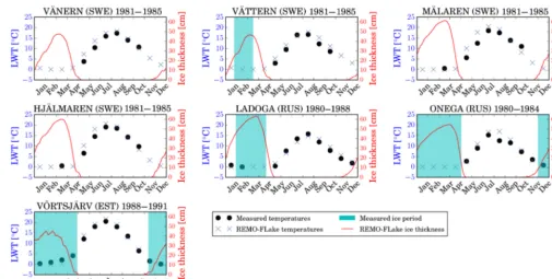
Lake temperatures in Sweden, Russia and Estonia are well captured by the model, as can be seen from Fig. 7. The model shows a small tendency to overestimate the lake tempera-tures, especially during spring. On the other hand, the au-tumn temperatures are well captured. The annual cycle is re-produced at all locations, although at Lake Onega the sum-mer peak is roughly 5◦C too high. Overall, the model gives realistic LWTs at all analyzed locations.
Figure 7 shows that the model overestimates the ice period length on all locations, except at Võrtsjärv, for which it is captured very well. At other locations, the start of the ice period is 1–2 months too early and the ice cover lasts roughly 1 month too long. The ice period definition issues are one part of the problem, but if we look at how much modeled ice is still present when the measurements show the end of the ice period, we can see that the values are still reasonably high (10–40 cm). This tends to indicate that the main problem is the cold bias in the model, especially when taking into account the too-early start of the ice season.
The ice period length analysis includes some error due to the definition problems already discussed in the previous sec-tion (how to define when a lake is ice free). In addisec-tion, the cold temperature bias over the large area of the domain in-creases the length of the modeled ice periods. The bias has an impact, especially over the lakes in Russia. Some of the error is also coming from the measurements. For example, for Lake Vättern, the ice period start time was calculated by using the mean of only two years (1981 and 1984; there were no other data for the years 1981–1985) and the start time dif-fered in these two years by 1 month. In addition, the timing of the ice period can be quite difficult and this difference could be an explaining factor for differences in spring LWTs. One would expect that due to the earlier end of the ice season in the measurements, the LWTs would be higher in the mea-surements than in the model results, but this is generally not the case; rather, REMO-FLake even tends to overestimate the LWTs. Also, the measurement location can play a role here; if it is close to the lakeshore, the modeled spring values will be underestimated and autumn time overestimated. However, there is no clear signal like this, which would indicate that the measurement location is not a crucial factor here.
4.3 Vertical profiles from specific lakes
We have also compared the vertical profiles of LWTs. The analysis has been done only for five Finnish lakes because measurement data were not available for all the locations an-alyzed in Sect. 4.1 (see Table S1). Measurements are done during summer from a boat and winter through ice. The fre-quency of measurement is usually three times per month and has some gaps during thin ice periods. This makes the mea-surement data frequency quite coarse compared to model data output frequency. Thus, we have filtered the model re-sults to match the same dates when the measurements were made. Additionally, as the measurements have some gaps, we have excluded from the analysis all mean values based on one or two measurement data points to avoid the artificial inflation of the weight of sparse data points.
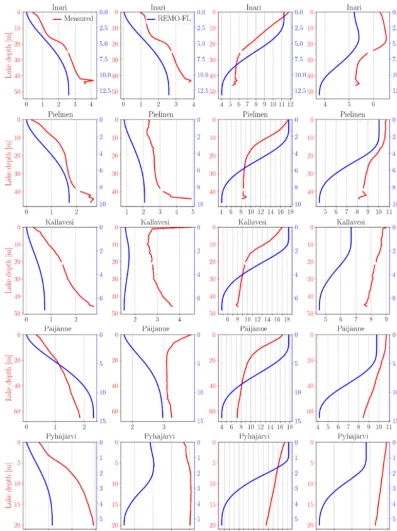
The calculation of the modeled vertical profiles is done by using the shape factor, mixing layer depth, mixing layer temperature and bottom temperature (details on these vari-able and the calculation method can be found in Mironov, 2008). During the ice period, FLake does not change the mix-ing layer depth; instead the last value before the ice period is used for the whole ice season. In the analysis, we have set the mixing layer depth to zero during the ice season and otherwise used the modeled depth. The mean depths of the lakes are similar in the model as in reality (see Table 2), but the maximum depths are not available from Choulga et al. (2014). Thus, in Fig. 8 the measurement depth and model lake depth are on separateyaxes. In this way, we can com-pare the shapes of the temperature profiles while also look-ing into the actual temperatures. However, as the depths dif-fer quite significantly, the profiles only indicate how well the model captures the measured values in the current depth setup. With more realistic depths, the profiles could change and this error source should be kept in mind.
Figure 7.Measured and modeled lake water temperatures (LWTs) and ice periods from Sweden, Russia and Estonia. The lake temperatures for Lake Ladoga are calculated only for the northern part (following the measurement approach), but the ice period and depth are for the whole lake.
are closer to the measured ones and overall the temperature difference stays within a few degrees.
During summer the profiles are fairly well captured. The measured and modeled surface temperatures are within 1– 2◦C at all locations, but the near-surface temperatures dif-fer at all locations. This is most probably caused by the as-sumed shape representation of the temperature profile in the model combined with different depths between the model and measurements. Also, the near-bottom temperatures have a cold bias, especially at Lake Pyhäjärvi, where it is almost 10◦C. This indicates that the bottom sediment temperature has some error, and a 35-year-long spin-up run was per-formed. The bottom temperatures are mainly lower in the model than in measurements at all locations and all seasons. This is somewhat surprising as the lakes are shallower in the model than in reality, and thus one could expect higher heat transfer from the atmosphere to the lake bottom in the model during open lake seasons. It is possible that the initial bottom temperatures, i.e., the deep soil temperature taken from the ERA-Interim data were, too cold and the spin-up time was too short to correct this. However, we see no drift in the lake bottom temperatures, which would suggest that this is not the reason.
The shapes of the temperature profiles during autumn are in reasonable accord with the measurements. The measured values are higher than the modeled ones at all locations. The near-surface values are within a couple of degrees, but the near-bottom temperatures differ by up to 5◦C. However,
despite the differences and uncertainties related to analysis coming from the different lake depths, the seasonally av-eraged vertical profiles are realistic and show that REMO– FLake has the capability to reproduce the vertical profiles of the lake temperatures.
5 Conclusions
In this work, the regional climate model REMO was in-teractively coupled with the lake model FLake (REMO– FLake). With the new version we have simulated the Fenno-Scandinavian climate over 35 years and evaluated the model in terms of climate- and lake-related variables. Fenno-Scandinavia has a large number of lakes of various sizes, making it a very suitable domain for a coupled regional–lake model. In addition, we have tested how sensitive the model is to different lake parameters and how much the snow albedo scheme influences the wintertime climate.
Figure 8. Vertical profiles of the measured and modeled seasonally averaged lake water temperatures (LWTs) in different lake depths. The values have been averaged for the time period of 1979–2015. The lake depth is shown for measurements (red color) and model results separately (blue color). Also, we have averaged the model results only over days when measurements were available because the measurement frequency was low (a few times per month).
FLake captures the Fenno-Scandinavian temperatures better than the original version. In terms of precipitation, REMO– FLake outperforms standard REMO in all seasons other than summer. During summer, the convective precipitation is too
active in REMO–FLake, leading to a wet bias over areas with a high lake density.
Finnish lakes. The results show that the model can capture the LWTs well, although there are some differences during spring due to the longer modeled ice period associated with the cold bias. The ice thicknesses tend to be overestimated, especially in areas where the cold bias is strongest. The snow thickness on ice also shows slight overestimation, which is caused either by the missing porous ice formation in FLake or the missing horizontal snow transport due to wind. Over-all, the model performs well in terms of the variables an-alyzed. We also did some LWT and ice depth analysis for lakes outside Finland. This analysis showed that the model performs very well throughout the Fenno-Scandinavian do-main. Ice depth and ice season length had some overestima-tions due to the cold bias in the model, but overall the differ-ences to measurements were small. The vertical lake temper-ature profiles were also analyzed and they showed that the modeled profiles have very similar features as the measured ones, while the modeled near-bottom temperatures are gen-erally underestimated.
We did not analyze in detail the reasons for the cold bias in this work. However, we did test how sensitive the model is to the snow albedo scheme, which is originally based on a snow temperature approach. We implemented another scheme originating from the Biosphere–Atmosphere Trans-fer Scheme (BATS), which takes into account the aging of snow, soot loading, grain size and the influence of solar zenith angle. Our test simulations shows that the snow albedo has only a minor impact on the cold bias. Although the snow albedos had differences between the two schemes, the impact on simulated climate is reduced by the rather low intensity of solar radiation during the snow season in Fenno-Scandinavia. A detailed analysis of the cold bias problem and the causes behind it will be left for forthcoming model development steps and publications. In particular, it would be worth look-ing at the representation of snow physics at land, includlook-ing snow heat conductivity. From a technical point of view, the computational costs of the implemented lake model are in-significant, thus further suggesting the use of the new model version.
Code availability. The source code for FLake is publicly avail-able (http://www.flake.igb-berlin.de/). The sources for REMO (and REMO–FLake) are available on request from the Climate Service Center Germany (contact@remo-rcm.de).
Appendix A: Ice cover period analysis
Table A1.Measured ice period start and end days (as the day of the year) and the length of the ice period in days. The differences to
modeled values are also shown (model–measurements; i.e., when the values are negative, the model is too early in its prediction and when the values are positive, the model is late in its prediction). If the difference between measured and modeled ice period start, end or length is less than 2 weeks, the values are boldfaced. The values have been averaged for the time period 1979–2015.
Measured Model Measured Model Measured Model
ice period start difference ice period end difference ice period length difference
Haukivesi 339 −15 127 7 154 22
Inari 313 −13 151 6 204 19
Kallavesi 340 −17 130 5 156 22
Lappajärvi 330 3 126 7 162 4
Näsijärvi 350 −22 123 3 139 25
Oulujärvi 326 −17 138 5 178 22
Pielinen 330 −14 134 8 170 22
Pyhäjärvi 342 −9 116 5 140 14
Päijänne 347 −13 123 12 142 25
The Supplement related to this article is available online at https://doi.org/10.5194/gmd-11-1321-2018-supplement.
Author contributions. JPP did the lake model coupling based on earlier work by JK and the coding work for lake tiles and snow albedo. JPP also planned the simulations, did major parts of the analysis and wrote the paper. TM and YG helped with the connec-tions between the main model and the lake model and tiles (in terms of soil and snow). KS and DJ assisted with the main model struc-ture (tiles) and physical processes. JK gave her expertise on water temperature and ice and snow thickness measurement data. PR gave his expertise on the snow albedo part and JA assisted with the lake temperature analysis. HK and AL assisted in the analysis and paper-writing phases and AL also initiated the work. The coauthors also helped with the paper by giving valuable comments.
Competing interests. The authors declare that they have no conflict of interest.
Special issue statement. This article is part of the special issue “Modelling lakes in the climate system (GMD/HESS inter-journal SI)”. It is a result of the 5th workshop on “Parameterization of Lakes in Numerical Weather Prediction and Climate Modelling”, Berlin, Germany, 16–19 October 2017.
Acknowledgements. The authors would like to thank Pentti Pirinen and Juha Aalto from the Weather and Climate Change Impact Research unit of the Finnish Meteorological Institute for providing the gridded data over Finland and helping with technical aspects. We also want to thank Otto Hyvärinen from the same unit for his help with the statistical analysis. We are grateful to Margaret Choulga from the Russian State Hydrometeorological University for providing the updated lake data. The insights about the FLake model by Dmitrii Mironov from the Deutscher Wetterdienst have been very valuable and the authors would like to express their gratitude. We also want to thank Aku Riihelf¨rom the Finnish Meteorological Institute for his help with the satellite albedo mea-surement data. We are also thankful for the insights regarding the snow albedo from Thomas Raddatz from the Max Planck Institute for Meteorology. We acknowledge the E-OBS dataset from the EU-FP6 project ENSEMBLES (http://ensembles-eu.metoffice.com) and the data providers in the ECA&D project (http://www.ecad.eu). Tiina Markkanen acknowledges the Academy of Finland Center of Excellence program (grant no. 307331) and EU LIFE12 project ENV/FI/000409. Hannele Korhonen acknowledges funding from the European Research Council (ERC) under the European Union Horizon 2020 research and innovation program under grant agreement no. 646857. The authors would like to thank Patrick Le Moigne from Météo-France and the anonymous referee for their valuable comments, which helped to improve the paper.
Edited by: David Lawrence
Reviewed by: Patrick Le Moigne and one anonymous referee
References
Aalto, J., Pirinen, P., and Jylhä, K.: New gridded daily climatology of Finland: Permutation-based uncertainty estimates and tempo-ral trends in climate, J. Geophys. Res.-Atmos., 121, 3807–3823, https://doi.org/10.1002/2015JD024651, 2016.
Arakawa, A. and Lamb, V.: Computational design and the basic dynamical processes of the UCLA general circulation Model, Methods in Computational Physics, 17, 173–265, 1977. Asselin, R.: Frequency filter for time integrations, Mon. Weather
Rev., 100, 487–490, 1972.
Bennington, V., Notaro, M., and Holman, K. D.: Improving Cli-mate Sensitivity of Deep Lakes within a Regional CliCli-mate Model and Its Impact on Simulated Climate, J. Climate, 27, 2886–2911, https://doi.org/10.1175/JCLI-D-13-00110.1, 2014.
Benson, B. and Magnuson, J.: Global Lake and River Ice Phe-nology Database, Version 1. Freeze/Thaw Dates, NSIDC: Na-tional Snow and Ice Data Center, Boulder, Colorado USA, https://doi.org/10.7265/N5W66HP8, last access: 10 February 2016, 2000 (updated 2012).
Brovkin, V., Boysen, L., Raddatz, T., Gayler, V., Loew, A., and Claussen, M.: Evaluation of vegetation cover and land-surface albedo in MPI-ESM CMIP5 simulations, J. Adv. Model. Earth Sy., 5, 48–57, https://doi.org/10.1029/2012MS000169, 2013. Choulga, M., Kourzeneva, E., Zakharova, E., and Doganovsky, A.:
Estimation of the mean depth of boreal lakes for use in numer-ical weather prediction and climate modelling, Tellus A, 66, 1, https://doi.org/10.3402/tellusa.v66.21295, 2014.
Davies, H. C.: A laterul boundary formulation for multi-level prediction models, Q. J. Roy. Meteor. Soc., 102, 405–418, https://doi.org/10.1002/qj.49710243210, 1976.
Dee, D. P., Uppala, S. M., Simmons, A. J., Berrisford, P., Poli, P., Kobayashi, S., Andrae, U., Balmaseda, M. A., Balsamo, G., Bauer, P., Bechtold, P., Beljaars, A. C. M., van de Berg, L., Bidlot, J., Bormann, N., Delsol, C., Dragani, R., Fuentes, M., Geer, A. J., Haimberger, L., Healy, S. B., Hersbach, H., Hólm, E. V., Isaksen, L., Kållberg, P., Köhler, M., Matricardi, M., McNally, A. P., Monge-Sanz, B. M., Morcrette, J.-J., Park, B.-K., Peubey, C., de Rosnay, P., Tavolato, C., Thépaut, J.-N., and Vitart, F.: The ERA-Interim reanalysis: configuration and perfor-mance of the data assimilation system, Q. J. Roy. Meteor. Soc., 137, 553–597, https://doi.org/10.1002/qj.828, 2011.
Dickinson, R. E., Henderson-Sellers, A., and Kennedy, P. J.: Biosphere-atmosphere Transfer Scheme (BATS) Version 1e as Coupled to the NCAR Community Climate Model, Tech. rep., National Center for Atmospheric Research, https://doi.org/10.5065/D67W6959, 1993.
FLake webpage: Lake Model FLake, available at: http://www.flake. igb-berlin.de/, last access: 12 January 2018.
Gao, Y., Markkanen, T., Backman, L., Henttonen, H. M., Pietikäinen, J.-P., Mäkelä, H. M., and Laaksonen, A.: Bio-geophysical impacts of peatland forestation on regional cli-mate changes in Finland, Biogeosciences, 11, 7251–7267, https://doi.org/10.5194/bg-11-7251-2014, 2014.
Gao, Y., Weiher, S., Markkanen, T., Pietikäinen, J.-P., Gregow, H., Henttonen, H., Jakob, D., and Laaksonen, A.: Implementation of the CORINE land use classification in the regional climate model REMO, Boreal Environ. Res., 20, 261–282, 2015.
Re-gional Climate Model: The Impact of the Great Lakes System on Regional Greenhouse Warming, J. Climate, 25, 7723–7742, https://doi.org/10.1175/JCLI-D-11-00388.1, 2012.
Hagemann, S.: An improved land surface parameter data set for global and regional climate models, Max Planck Institute for Meteorology report series, Hamburg, Germany, Report No. 336, 2002.
Hagemann, S. and Gates, L. D.: Improving a subgrid runoff param-eterization scheme for climate models by the use of high resolu-tion data derived from satellite observaresolu-tions, Clim. Dynam., 21, 349–359, https://doi.org/10.1007/s00382-003-0349-x, 2003. Haylock, M. R., Hofstra, N., Klein Tank, A. M. G., Klok, E. J.,
Jones, P. D., and New, M.: A European daily high-resolution gridded data set of surface temperature and precipitation for 1950–2006, J. Geophys. Res.-Atmos., 113, D20119, https://doi.org/10.1029/2008JD010201, 2008.
Hostetler, S. W. and Bartlein, P. J.: Simulation of lake evaporation with application to modeling lake level variations of Harney-Malheur Lake, Oregon, Water Resour. Res., 26, 2603–2612, https://doi.org/10.1029/WR026i010p02603, 1990.
ILEC: International Lake Environmental Committee. Survey of the State of World Lakes. Data Books of the World Lake Environ-ments, Vols. 15. ILEC/UNEP Publications, Otsu, Japan, avail-able at: http://wldb.ilec.or.jp (last access: 20 March 2018), 1988– 1993.
Jacob, D.: A note to the simulation of the annual and inter-annual variability of the water budget over the Baltic Sea drainage basin, Meteorol. Atmos. Phys., 77, 61–73, https://doi.org/10.1007/s007030170017, 2001.
Jacob, D. and Podzun, R.: Sensitivity studies with the regional climate model REMO, Meteorol. Atmos. Phys., 63, 119–129, https://doi.org/10.1007/BF01025368, 1997.
Karlsson, K.-G., Riihelä, A., Müller, R., Meirink, J. F., Sedlar, J., Stengel, M., Lockhoff, M., Trentmann, J., Kaspar, F., Holl-mann, R., and Wolters, E.: CLARA-A1: CM SAF cLouds, Albedo and Radiation dataset from AVHRR data – Edition 1 – Monthly Means/Daily Means/Pentad Means/Monthly His-tograms, Satellite Application Facility on Climate Monitoring, https://doi.org/10.5676/EUM_SAF_CM/CLARA_AVHRR/V001, 2012.
Karlsson, K.-G., Anttila, K., Trentmann, J., Stengel, M., Fokke Meirink, J., Devasthale, A., Hanschmann, T., Kothe, S., Jääskeläinen, E., Sedlar, J., Benas, N., van Zadelhoff, G.-J., Schlundt, C., Stein, D., Finkensieper, S., Håkansson, N., and Hollmann, R.: CLARA-A2: the second edition of the CM SAF cloud and radiation data record from 34 years of global AVHRR data, Atmos. Chem. Phys., 17, 5809–5828, https://doi.org/10.5194/acp-17-5809-2017, 2017.
Kirillin, G., Leppäranta, M., Terzhevik, A., Granin, N., Bern-hardt, J., EngelBern-hardt, C., Efremova, T., Golosov, S., Palshin, N., Sherstyankin, P., Zdorovennova, G., and Zdorovennov, R.: Physics of seasonally ice-covered lakes: a review, Aquat. Sci., 74, 659–682, https://doi.org/10.1007/s00027-012-0279-y, 2012. Kotlarski, S.: A Subgrid Glacier Parameterisation for Use in Re-gional Climate Modelling, PhD thesis, Max Planck Institute for Meteorology, Hamburg, Germany, Reports on Earth System Sci-ence, No. 42, 2007.
Kotlarski, S., Keuler, K., Christensen, O. B., Colette, A., Déqué, M., Gobiet, A., Goergen, K., Jacob, D., Lüthi, D., van
Meij-gaard, E., Nikulin, G., Schär, C., Teichmann, C., Vautard, R., Warrach-Sagi, K., and Wulfmeyer, V.: Regional climate model-ing on European scales: a joint standard evaluation of the EURO-CORDEX RCM ensemble, Geosci. Model Dev., 7, 1297–1333, https://doi.org/10.5194/gmd-7-1297-2014, 2014.
Kourzeneva, E., Martin, E., Batrak, Y., and Moigne, P. L.: Climate data for parameterisation of lakes in Nu-merical Weather Prediction models, Tellus A, 64, 1, https://doi.org/10.3402/tellusa.v64i0.17226, 2012.
León, L., Lam, D., Schertzer, W., Swayne, D., and Im-berger, J.: Towards coupling a 3D hydrodynamic lake model with the Canadian Regional Climate Model: Simulation on Great Slave Lake, Environ. Modell. Softw., 22, 787–796, https://doi.org/10.1016/j.envsoft.2006.03.005, 2007.
Louis, J.-F.: A parametric model of vertical eddy fluxes in the atmosphere, Bound.-Lay. Meteorol., 17, 187–202, https://doi.org/10.1007/BF00117978, 1979.
Loveland, T. R., Reed, B. C., Brown, J. F., Ohlen, D. O., Zhu, Z., Yang, L., and Merchant, J. W.: Development of a global land cover characteristics database and IGBP DISCover from 1 km AVHRR data, Int. J. Remote Sens., 21, 1303–1330, https://doi.org/10.1080/014311600210191, 2000.
Mallard, M. S., Nolte, C. G., Bullock, O. R., Spero, T. L., and Gula, J.: Using a coupled lake model with WRF for dynam-ical downscaling, J. Geophys. Res.-Atmos., 119, 7193–7208, https://doi.org/10.1002/2014JD021785, 2014.
Manabe, S.: Climate and the ocean circulation 1: I. The at-mospheric circulation and the hydrology of earth’s surface, Mon. Weather Rev., 97, 739–774, https://doi.org/10.1175/1520-0493(1969)097<0739:CATOC>2.3.CO;2, 1969.
Martynov, A., Sushama, L., and Laprise, R.: Simulation of temper-ate freezing lakes by one-dimensional lake models: performance assessment for interactive coupling with regional climate mod-els, Boreal Environ. Res., 15, 143–164, 2010.
Martynov, A., Sushama, L., Laprise, R., Winger, K., and Dugas, B.: Interactive lakes in the Canadian Regional Climate Model, ver-sion 5: the role of lakes in the regional climate of North Amer-ica, Tellus A, 64, 1, https://doi.org/10.3402/tellusa.v64i0.16226, 2012.
Mironov, D. V.: Parameterization of lakes in numerical weather pre-diction. Description of a lake model., Tech. Rep. 11, COSMO, Deutscher Wetterdienst, Offenbach am Main, Germany, 41 pp., 2008.
Mironov, D., Heise, E., Kourzeneva, E., Ritter, B., Schneider, N., and Terzhevik, A.: Implementation of the lake parameterisa-tion scheme FLake into the numerical weather predicparameterisa-tion model COSMO, Boreal Environ. Res., 15, 218–230, 2010.
Mironov, D., Ritter, B., Schulz, J.-P., Buchhold, M., Lange, M., and Machulskaya, E.: Parameterisation of sea and lake ice in numeri-cal weather prediction models of the German Weather Service, Tellus A, 64, 1, https://doi.org/10.3402/tellusa.v64i0.17330, 2012.