www.geosci-model-dev.net/4/993/2011/ doi:10.5194/gmd-4-993-2011
© Author(s) 2011. CC Attribution 3.0 License.
Geoscientific
Model Development
Plant functional type mapping for earth system models
B. Poulter1,2, P. Ciais2, E. Hodson1, H. Lischke1, F. Maignan2, S. Plummer3, and N. E. Zimmermann1
1Swiss Federal Research Institute WSL, Dynamic Macroecology, Z¨urcherstrasse 111, Birmensdorf 8903, Switzerland 2Laboratoire des Sciences du Climat et de L’Environment, UMR8212, CNRS – CEA, UVSQ, Gif-sur Yvette, France 3IGBP-ESA Joint Projects Office, c/o ESA-ESRIN, European Space Agency, Via Galileo Galilei, 00044, Frascati, Italy Received: 26 July 2011 – Published in Geosci. Model Dev. Discuss.: 26 August 2011
Revised: 4 November 2011 – Accepted: 8 November 2011 – Published: 16 November 2011
Abstract. The sensitivity of global carbon and water cycling to climate variability is coupled directly to land cover and the distribution of vegetation. To investigate biogeochemistry-climate interactions, earth system models require a represen-tation of vegerepresen-tation distributions that are either prescribed from remote sensing data or simulated via biogeography models. However, the abstraction of earth system state vari-ables in models means that data products derived from re-mote sensing need to be post-processed for model-data as-similation. Dynamic global vegetation models (DGVM) rely on the concept of plant functional types (PFT) to group shared traits of thousands of plant species into usually only 10–20 classes. Available databases of observed PFT dis-tributions must be relevant to existing satellite sensors and their derived products, and to the present day distribution of managed lands. Here, we develop four PFT datasets based on land-cover information from three satellite sensors (EOS-MODIS 1 km and 0.5 km, SPOT4-VEGETATION 1 km, and ENVISAT-MERIS 0.3 km spatial resolution) that are merged with spatially-consistent K¨oppen-Geiger climate zones. Us-ing a beta (ß) diversity metric to assess reclassification simi-larity, we find that the greatest uncertainty in PFT classifica-tions occur most frequently between cropland and grassland categories, and in dryland systems between shrubland, grass-land and forest categories because of differences in the mini-mum threshold required for forest cover. The biogeography-biogeochemistry DGVM, LPJmL, is used in diagnostic mode with the four PFT datasets prescribed to quantify the effect of land-cover uncertainty on climatic sensitivity of gross pri-mary productivity (GPP) and transpiration fluxes. Our re-sults show that land-cover uncertainty has large effects in arid regions, contributing up to 30 % (20 %) uncertainty in the sensitivity of GPP (transpiration) to precipitation. The
Correspondence to: B. Poulter ([email protected])
availability of PFT datasets that are consistent with current satellite products and adapted for earth system models is an important component for reducing the uncertainty of terres-trial biogeochemistry to climate variability.
1 Introduction
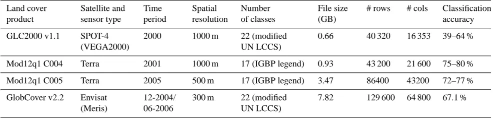
Table 1. Characteristics of the remotely sensed land cover datasets used to develop the phenology, physiognomy, and natural/managed traits for the PFT mapping.
Land cover product Satellite and sensor type Time period Spatial resolution Number of classes File size (GB)
# rows # cols Classification
accuracy
GLC2000 v1.1 SPOT-4
(VEGA2000)
2000 1000 m 22 (modified
UN LCCS)
0.66 40 320 16 353 39–64 %
Mod12q1 C004 Terra 2001 1000 m 17 (IGBP legend) 0.93 43 200 21 600 75–80 %
Mod12q1 C005 Terra 2005 500 m 17 (IGBP legend) 3.47 86400 43200 72–77 %
GlobCover v2.2 Envisat
(Meris)
12-2004/ 06-2006
300 m 22 (modified
UN LCCS)
7.82 129 600 64 800 67.1 %
There are now several (Table 1) moderate resolution global land-cover datasets available from different satellite sensors and research groups (Friedl et al., 2002, 2010; Bartholome and Belward, 2005; Arino et al., 2008) providing an oppor-tunity to assess ensemble variability. Although these land-cover datasets provide new opportunities for model-data as-similation studies to assess the effects of land-cover feed-backs (Quaife et al., 2008; Sterling and Ducharne, 2008; Jung et al., 2007), their approach for classifying land cover is not yet consistent with Earth System Model (ESM) re-quirements. This is because the concept of plant functional types used in ESMs cannot be mapped directly using re-mote sensing data since PFT traits represent a combination of spectral relationships, and climatic, ecological, and the-oretical assumptions (Smith et al., 1997; Sun et al., 2008; Running et al., 1995; Ustin and Gamon, 2010). The PFT concept consists of aggregating multiple species traits, al-lowing for the reduction of thousands of species to a small set of functional groups (typically<15) defined by their phe-nology type, physiognomy, photosynthetic pathway, and cli-mate zone. The advantage of the PFT classification system is that it allows the possibility for posing testable hypotheses that are feasible at global and centennial scales (Smith et al., 1997).
Existing PFT datasets include those by Bonan et al. (2002) for the Community Land Model, with updates from (Lawrence and Chase, 2007), by Verant et al. (2004) for the Orchidee DGVM, and by Lapola et al. (2008) for the SSiB model. Improvements to these PFT datasets are currently needed to expand the availability of land-cover datasets to al-low consistency with a more complete set of satellite sensors and more detailed or revised climate zone data, and to take into account current human land-use patterns. For example, Bonan et al. (2002) used multiple data sources to combine the IGBP-DISCover Global Land Cover Classification data (IGBP GLCC) and phenology-type data (from 1992–1993 AVHRR data) with vegetation continuous fields from De-Fries et al. (2000). They assigned biome types from biocli-matic definitions provided by Prentice et al. (1992) based on
gridded climate data from Legates and Wilmott (1990), cre-ating one of the first ESM-relevant PFT legends (Table 2) for the Community Land Model 3.0 (Dickinson et al., 2006). In comparison, Verant et al. (2004) combined simplified Olson biomes with IGBP GLCC data to create a PFT map for the Orchidee DGVM (Krinner et al., 2005). Lapola et al. (2008) developed a global PFT map by reclassifying legends from Olson et al. (1983) and Matthews (1983) and filling areas of mismatch with regional land cover information. A different PFT legend accompanies the MODIS land cover product us-ing categories defined by Runnus-ing et al. (1995) and has been developed from GLC2000 (Wang et al., 2006). For these particular PFT legends, the classifications include phenology type but not the associated climate zone, which is needed to assign climate-specific physiological parameters to each PFT (i.e., Sitch et al., 2003). As a consequence, vegeta-tion models using these particular PFT datasets must assume that biochemical and biophysical PFT parameters are con-stant globally across different climate zones (e.g., see Alton et al., 2009).
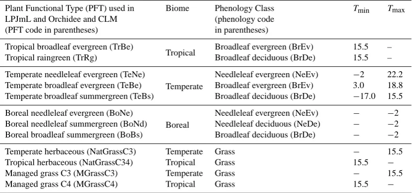
Table 2. Plant functional types (PFT) used in the Orchidee, LPJ and CLM dynamic global vegetation models. The PFTs are defined by
biome and by phenology, followed by temperature criteria (here shown from Sitch et al., 2003) for establishment (Tmin/Tmax, in◦C, are
calculated from twenty year annual means).
Plant Functional Type (PFT) used in LPJmL and Orchidee and CLM (PFT code in parentheses)
Biome Phenology Class
(phenology code in parentheses)
Tmin Tmax
Tropical broadleaf evergreen (TrBe)
Tropical Broadleaf evergreen (BrEv) 15.5 –
Tropical raingreen (TrRg) Broadleaf deciduous (BrDe) 15.5 –
Temperate needleleaf evergreen (TeNe)
Temperate
Needleleaf evergreen (NeEv) −2 22.2
Temperate broadleaf evergreen (TeBe) Broadleaf evergreen (BrEv) 3.0 18.8
Temperate broadleaf summergreen (TeBs) Broadleaf deciduous (BrDe) −17.0 15.5
Boreal needleleaf evergreen (BoNe)
Boreal
Needleleaf evergreen (NeEv) − −2
Boreal needleleaf summergreen (BoNd) Needleleaf deciduous (NeDe) − −2
Boreal broadleaf summergreen (BoBs) Broadleaf deciduous (BrDe) − −2
Temperate herbaceous (NatGrassC3) Temperate Grass − 15.5
Tropical herbaceous (NatGrassC34) Tropical Grass 15.5 −
Managed grass C3 (MGrassC3) Temperate Grass − 15.5
Managed grass C4 (MGrassC4) Tropical Grass 15.5 −
2 Methods
2.1 Land cover and climate zone datasets
Land-cover datasets, described in Table 1, were manually re-classified to PFT specific phenology type and physiognomic categories. The resulting categories were merged with cli-mate zones defined by the K¨oppen-Geiger classification sys-tem to resolve to PFT classes. The merged dataset was aggre-gated to 0.5◦spatial resolution (corresponding to the climate
and soils data used in LPJmL), representing the fractional abundance of PFT mixtures within a grid cell. All analyses were conducted at the global scale in Plate-Carr´ee (WGS84) projection, area correcting grid cells during post-processing when necessary. The original land-cover datasets varied in spatial resolution, time period of data collection, classifica-tion approach, and accuracy and are discussed below.
The K¨oppen-Geiger dataset was created by Peel et al. (2007) from over 4000 metrological stations contained in the Global Historical Climatological Network v2.0 database. The authors calculated climate indices (i.e., seasonal means, minimums, and maximums) for the stations from precipita-tion and temperature for their entire time series (mostly, the 20th century) and then interpolated to a 0.1◦resolution grid (not accounting for elevation). These indices were classified into one of 32 possible climate zones (Table 3) according to the original K¨oppen-Geiger classification system (K¨oppen, 1936).
The GLC2000 land-cover data were generated from SPOT-VEGETATION (SPOT 4) and ATSR-2/DMSP sensors and are available for most of the vegetated surface of the globe (75◦N to 56◦S, excluding Antarctica) at 1 km
resolu-tion (Bartholome and Belward, 2005; Hugh et al., 2004). The data were collected between November 1999 and December 2000. The GLC2000 classification (Table 4) was conducted by regional expert groups following an unsupervised clas-sification of 19 similar geographic regions using the LCCS nomenclature (22 categories for global purposes).
The GlobCover data became available in 2008 (Arino et al., 2008) and represent the highest-spatial resolution data available for global extent at this time (0.3 km resolution). The classification system also follows the LCCS system (22 categories, Table 5) and the spectral data were acquired from the MERIS sensor on-board the ENVISAT satellite be-tween June 2004 and December 2006. Individual pixels are classified using unsupervised and supervised approaches on sub-global regional clusters.
Table 3. K¨oppen-Geiger biome types (Code column is defined in Peel et al., 2007) and their simplified equivalents required for DGVM PFT
classification. WhereThotandTcoldare temperature of the hottest and coldest month (◦C), and MAT is mean annual temperature (◦C).
Number Code K¨oppen-Geiger biome category PFT biome equivalent
(this study)
1 Af Tropical Tcold=>18 Tropical
2 Am
3 Aw
4 BWh Arid MAT =>18
5 BWk MAT<18 Temperate (warm)
6 BSh MAT =>18 Tropical
7 BSk MAT<18 Temperate (warm)
8 Csa Temperate
Thot>10
&Tcold<18
Thot=>22 Temperate (warm)
9 Csb Temperate (cool)
10 Csc
11 Cwa Thot=>22 Temperate (warm)
12 Cwb Temperate (cool)
13 Cwc
14 Cfa Thot=>22 Temperate (warm)
15 Cfb Temperate (cool)
16 Cfc
17 Dsa Cold
Thot>10
&Tcold<0
Thot=>22 Boreal (warm)
18 Dsb Boreal (cool)
19 Dsc
20 Dsd
21 Dwa Thot=>22 Boreal (warm)
22 Dwb Boreal (cool)
23 Dwc
24 Dwd
25 Dfa Thot=>22 Boreal (warm)
26 Dfb Boreal (cool)
27 Dfc
28 Dfd
29 ET Polar
Thot<10
Thot>0
30 EF Thot<0
31==29 ETH
32==30 EFH
2.2 Reclassifying the legends
The land-cover data were first cross-walked (reclassified) to a phenology-based legend consistent with the plant functional types used in major DGVM and land surface models (Ta-ble 2). Figure 1 illustrates the flow of data processing, with the merging of the phenology type and climate data described in the following section. Manually reclassifying legends is inherently subjective, especially with the treatment of mixed vegetation categories where multiple possible classes must
Table 4. The GLC2000 legend (based on LCCS) and corresponding DGVM phenology class (from Table 2).
GLC ID GLC2000 description DGVM phenology class
1 Tree Cover, broadleaved, evergreen 90 % BrEv, 10 % NatGrass
2 Tree Cover, broadleaved, deciduous, closed 100 % BrDe
3 Tree Cover, broadleaved, deciduous, open (open 15–40 % tree cover) 80 %BrDe, 20 % NatGrass
4 Tree Cover, needle-leaved, evergreen 100 % NeEv
5 Tree Cover, needle-leaved, deciduous 100 % NeDe
6 Tree Cover, mixed leaf type 25 % BrEv, BrDe, NeEv, NeDe
7 Tree Cover, regularly flooded, fresh water (& brackish) 25 % BrEv, BrDe, NeEv, NeDe
8 Tree Cover, regularly flooded, saline water 25 % BrEv, BrDe, NeEv, NeDe
9 Mosaic: Tree cover/Other natural vegetation 20 % BrEv, BrDe, NeEv, NeDe, NatGrass
10 Tree Cover, burnt 25 % BrEv, BrDe, NeEv, NeDe
11 Shrub Cover, closed-open, evergreen 40 % BrEv, NeEv, 20 % NatGrass
12 Shrub Cover, closed-open, deciduous 80 % BrDe, 20 % NatGrass
13 Herbaceous Cover, closed-open 100 % NatGrass
14 Sparse Herbaceous or sparse Shrub Cover 60 % NatGrass, 40 % bare
15 Regularly flooded Shrub and/or Herbaceous Cover 10 % BrEv, BrDe, NeEv, NeDe, 60 % NatGrass
16 Cultivated and managed areas 100 % ManGrass
17 Mosaic: Cropland/Tree Cover/Other natural vegetation 8 % BrEv, BrDe, NeEv, NeDe, NatGrass, ManGrass
18 Mosaic: Cropland/Shrub or Grass Cover 8 % BrEv, BrDe, NeEv, NeDe, NatGrass, ManGrass
19 Bare Areas Bare
20 Water Bodies (natural & artificial) Water
21 Snow and Ice (natural & artificial) Bare
22 Artificial surfaces and associated areas Urban
23 No data No data
Table 5. The GlobCover legend (LCCS) and corresponding DGVM phenology class (from Table 2).
ID GlobCover description DGVM phenology class
11 Post-flooding or irrigated croplands (or aquatic) 100 % ManGrass
14 Rainfed croplands 100 % ManGrass
20 Mosaic cropland (50–70 %)/vegetation (grassland/shrubland/forest) (20–50 %)
10 % BrEv, BrDe, NeEv, NeDe, Nat-Grass, 50 % ManGrass
30 Mosaic vegetation (grassland/shrubland/forest) (50–70 %) / cropland (20–50 %)
10 % BrEv, BrDe, NeEv, NeDe, 20 % NatGrass, 40 % ManGrass
40 Closed to open (>15 %) broadleaved evergreen or semi-deciduous forest (>5 m)
50 % BrEv, BrDe
50 Closed (>40 %) broadleaved deciduous forest (>5 m)
100 % BrDe
60 Open (15–40%) broadleaved deciduous forest/woodland (>5 m)
80 % BrDe, 20 % NatGrass
70 Closed (>40 %) needleleaved evergreen forest (>5m)
100 % NeEv
90 Open (15–40 %) needleleaved deciduous or evergreen forest (>5 m)
40 % NeEv, NeDe, 20 % NatGrass
100 Closed to open (>15 %) mixed broadleaved and needleleaved forest (>5 m)
25 % BrEv, BrDe, NeEv, NeDe
110 Mosaic forest or shrubland (50–70 %)/grassland (20–50 %)
20 % BrEv, BrDe, NeEv, NeDe, Nat-Grass
120 Mosaic grassland (50–70 %)/forest or shrubland (20–50 %)
10 % BrEv, BrDe, NeEv, NeDe, 60 % NatGrass
130 Closed to open (>15 %) (broadleaved or needleleaved, evergreen or deciduous) shrubland (<5 m)
20 % BrEv, NeEv, 10 % BrDe, NeDe, 40 % NatGrass
140 Closed to open (>15 %) herbaceous vegetation (grassland, savannas or lichens/mosses)
20 % NeEv, 80 % NatGrass
150 Sparse (<15 %) vegetation 40 % NatGrass, 60 % bare
160 Closed to open (>15 %) broadleaved forest regularly flooded (semi-permanently or temporarily) – Fresh or brackish water
33 % BrEv, BrDe, NatGrass
170 Closed (>40 %) broadleaved forest or shrubland permanently flooded – Saline or brackish water
50 % BrEv, BrDe
180 Closed to open (>15 %) grassland or woody vegetation on regularly flooded or waterlogged soil – Fresh, brackish or saline water
20 % BrEv, BrDe, NeEv, NeDe, NatGrass
190 Artificial surfaces and associated areas (Urban areas>50 %)
100 % Urban
200 Bare areas 100 % Bare
210 Water bodies 100 % Water
220 Permanent snow and ice 100 % Bare
230 No data (burnt areas, clouds,. . . ) 100 % No data
Tables 4, 5, and 6 list the original land-cover classes from GLC2000, GlobCover, and MODIS and their corresponding reclassification into phenology type (Table 2). Six PFT-specific phenology-type/physiognomy classes were pre-defined, corresponding with categories used in several DGVM models (broadleaf evergreen BrEv, broadleaf de-ciduous BrDe, needleaf evergreen NeEv, needleleaf
single PFT phenology/physiognomy class. In these cases, the land cover class was reclassified to one of several possible phenology-types and physiognomy classes whose probabil-ity was assigned by assessing the supplementary data regard-ing the legend definitions or examinregard-ing the spatial pattern of observed land cover classes, and based on expert opinion on how the class might be composed of various phenology types (similar to Wang et al., 2006). In these cases, for ex-ample, a “mixed tree cover” category would yield 25 % equal probability (using a uniform distribution for all mixed land cover categories) with the grid cell being reclassified to ei-ther BrEv, BrDe, NeEv, or NeDe. This approach resulted in a single category cell, but when the cells were aggregated to coarser resolution (described below), the relative PFT frac-tions more realistically represented the original mixed for-est classes (for example, aggregating from 1 km mixed forfor-est category to 0.5 degree resolution results in 0.5 degree frac-tions equal to 0.25 for BrEv, BrDe, NeEv, and NeDe, sum-ming to 1.0 for an aggregated cell).
2.3 Merging and aggregating phenology and climate zones
The K¨oppen-Geiger dataset was first adjusted to expand its coastal grid cell definitions to neighboring ocean grid cells to allow a complete overlay of land cover with climate zone. The buffered K¨oppen-Geiger data were then downscaled to the spatial resolution of the corresponding land-cover dataset using a nearest neighbor resampling algorithm. The resam-pled K¨oppen-Geiger data were reclassified into one of three major biome types (following the rules described in Table 3), namely: tropical, temperate and boreal. The temperate and the boreal biome were further subdivided into either cool (<22◦C) or warm (=>22◦C) types to distinguish between C3 or C4 photosynthesis in the former, and temperate needle-leaf and broadneedle-leaf trees in the latter (based on their PFT temperature establishment thresholds in Table 2). While C4 grasses can establish at cooler temperatures (i.e., the LPJ model uses a temperature of 15◦C, Table 2), this tempera-ture threshold (22◦C) has been shown in prior studies to be a critical “crossover” temperature for C3 and C4 adaptations (Collatz et al., 1998).
Each of the 4 reclassified phenology type datasets were then merged with the climate zones to produce the final PFT classification at the spatial resolution of the original land cover data following the assembly rules in Table 7. Some exceptions were made to account for the full combination of phenology and climate zone possibilities. For example, because there are few to no deciduous needleleaf PFTs ob-served in tropical and temperate ecosystems, this phenology type was treated as tropical broadleaf raingreen (deciduous) or temperate broadleaf summergreen PFT. Natural and man-aged grasslands were split into the C3 and C4 photosynthetic pathways according to temperature thresholds that defined tropical versus temperate, and cool versus warm temperate
biomes from the K¨oppen-Geiger data. This approach may underestimate C3/C4 grass mixtures or C4 summer crops (i.e., maize) that might be planted in cooler regions (Ra-mankutty and Foley, 1998).
The PFT classifications were aggregated to a spatial reso-lution of 0.5◦by summing the area of each PFT class within the corresponding 0.5◦cell (16 classes, Table 7) and divid-ing by the grid cell area. A spatial resolution of 0.5◦ was chosen for this study because most models in the ESM com-munity use climate and other ancillary driver (e.g., soil type) data at this resolution, or greater (Zobler, 1986;New et al., 2002). The aggregation of PFT fractions can also be carried out at finer resolution, but at smaller window sizes the es-timates of fractional PFT coverage may become more sen-sitive to the selection of probability distribution. Each of the four PFT fractional abundance files were filtered with a global land/water mask, which was derived from a global soils database (Zobler, 1986). This ensured that the terrestrial surface area and land/ocean boundaries were equal between datasets.
2.4 Measuring PFT agreement
We analyzed the agreement between PFT fractional abun-dance (and re-groupings of PFTs by various traits) with a beta (ß) diversity metric (mean Euclidean distance) calcu-lated for each grid cell. Euclidean distance is a measure of dissimilarity between groups with multiple members (Leg-endre et al., 2005) and is commonly used to summarize land-scape species diversity from multiple sampling plots (Whit-taker, 1972). In our case, the “plots” were the grid cells which contained the fractional PFT abundances contained from the different classification datasets. This analysis had two objectives; the first was to assess, geographically, where regions of high uncertainty in PFT abundance may exist, the second was to help evaluate the methods for the reclassifi-cation of legends, especially for the mixed vegetation cate-gories.
The beta diversity metric was calculated for each grid cell for each of the four datasets, for the standard PFT classifica-tion, and for three re-groupings based on PFT traits. These regroupings were 1. Phenology type (total evergreen ver-sus total deciduous fraction), 2. Physiognomy (total woody versus total herbaceous fraction), and 3. Management status (natural grass versus managed grass). Equation (1) presents the variables used for calculating the Euclidean distance, the mean of which, we consider to represent beta diversity, ß. For every grid cell c, the Euclidean distance, D was calculated between every combination of classifications, N (1. . . 4) composed of 10 PFTs (I= 10) and their correspond-ing fractional abundanceAfor the different classifications (j andk).
ßc=Dc= N P n=1 I P i=1
Ai,j,c−Ai,k,c2 0.5
Table 6. Modis collection 4 and 5 legend (IGBP) and corresponding DGVM phenology class (from Table 2). For mixed phenology cells, it was assumed that any phenology type could be found, these were determined randomly using a uniform distribution.
MODIS ID MODIS description DGVM phenology class
0 Water 100 % Water
1 Evergreen Needleleaf Forest 100 % NeEv
2 Evergreen Broadleaf Forest 100 % BrEv
3 Deciduous Needleleaf Forest 100 % NeDe
4 Deciduous Broadleaf Forest 100 % BrDe
5 Mixed Forests 25 % BrEv, BrDe, NeEv, NeDe
6 Closed Shrublands 10 %, BrEv, BrDe, 30 % NeEv, 10 % NeDe, 40 % NatGrass 7 Open Shrublands 10 % BrEv, BrDe, NeDe, NeEv, 20 % NatGrass, 40 % Bare 8 Woody Savannas 20 %, BrEv, 10 % BrDe, 20 % NeEv, 50 % NatGrass
9 Savannas 10 %, BrEv, 20 % NeEv, 70 % NatGrass
10 Grasslands 100 % NatGrass
11 Permanent Wetlands 20 % BrEv, BrDe, NeEv, NeDe, NatGrass
12 Croplands 100 % ManGrass
13 Urban and Built-Up 100 % Urban
14 Cropland/Natural Vegetation Mosaic 8 % BrEv, BrDe, NeEv, NeDe, NatGrass, ManGrass
15 Snow and Ice 100 % Bare
16 Barren or Sparsely Vegetated (<10 % veg. cover) 10 % NatGrass, 90 % Bare 17 (IGBP Water Bodies, recoded to 0 for MODIS Land Product consistency.) 100 % Water
254 Unclassified 100 % No data
255 Fill Value 100 % No data
Table 7. Final merging rules for phenology and climate zone, and legend for final PFT map (including non-PFT categories).
Biome Phenology PFT Category Data Band
Tropical Broadleaf evergreen Tropical Broadleaf Evergreen 1
Tropical Broadleaf deciduous Needleleaf deciduous Tropical Broadleaf Raingreen 2 Tropical Temperate (warm) Temperate (cool) Boreal (warm) Needleaf evergreen Temperate Needleleaf Evergreen 3 Temperate (warm) Temperate (cool) Boreal (warm) Boreal (cool) Broadleaf evergreen Temperate Broadleaf Evergreen 4 Temperate (cool) Temperate (warm) Boreal (warm) Broadleaf deciduous Needleleaf deciduous Temperate Broadleaf Summergreen 5
Boreal (cool) Needleleaf evergreen Boreal Needleleaf Evergreen 6
Temperate (cool) Boreal (cool) Needleleaf deciduous Boreal Needleleaf Deciduous 7
Boreal (cool) Broadleaf deciduous Boreal Broadleaf Summergreen 8
Temperate (cool) Boreal (warm) Boreal (cool) Natural Grass Natural grassland C3 9
Tropical Temperate (warm) Natural Grass Natural grassland C4 10
Temperate (cool) Boreal (warm) Boreal (cool) Managed Grass Managed grassland C3 11
Tropical Temperate (warm) Managed Grass Managed grassland C4 12
Non-vegetated
Barren/Bare 13
Water 14
Urban 15
No Data 16
The mean Euclidean distance (beta diversity) between groups (Dc)was calculated as the mean of the diagonals from the resulting matrix to represent overall dissimilarity (Legendre et al., 2005; Whittaker, 1972). The variance of the Euclidean distance matrix was also calculated using the same approach, but taking the variance of the matrix diagonals rather than the mean. The two approaches were used to aggregate the distance matrix into a single index as recommended by Leg-endre et al. (2005). ß was plotted as both geographic maps and as latitudinal summaries to explore the spatial patterns of uncertainty for each grouping.
An ordination analysis was conducted for four individual grid cells representative of major biomes (temperate, tropi-cal, boreal, and desert) to investigate the similarity between PFT products and to display the main gradients partitioning
them. The PFT products included those developed in this study, the existing products described in the Introduction for Orchidee and CLM, and the results from a DGVM simula-tion from LPJmL (described below). Non-metric multidi-mensional scaling (NMDS) was chosen (using a Euclidean distance matrix); this ordination method is less sensitive to non-linear relationships among variables.
2.5 Prescribing PFT data to a dynamic global vegetation model
Table 8. Global plant functional type and non-vegetated cover (%) for land surface.
PFT GLC2000 Globcover Modis C004 Modis C005 StDev
Tropical Broadleaf Evergreen 7.97 6 11.47 11.13 2.62
Tropical Broadleaf Raingreen 7.52 8.96 2.71 3.15 3.13
Temperate Needleleaf Evergreen 3.68 5.68 5.32 5.6 0.94
Temperate Broadleaf Evergreen 2.86 3.3 5.24 5.22 1.25
Temperate Broadleaf Summergreen 5.51 5.38 3.08 3.22 1.33
Boreal Needleleaf Evergreen 5.78 5.24 5.77 5.62 0.25
Boreal Needleleaf Deciduous 3.87 4.05 2.45 3.78 0.73
Boreal Broadleaf Summergreen 4.05 3.09 2.39 2.47 0.77
Natural grassland C3 7.45 7.7 7.56 8.04 0.26
Natural grassland C4 13.87 11.21 17.99 19.13 3.67
Managed grassland C3 5.01 3.92 5.26 5.14 0.62
Managed grassland C4 8.56 8.83 4.87 4.95 2.19
Unvegetated (ice/barren, urban, water, no data)
23.88 26.62 25.87 22.55 1.80
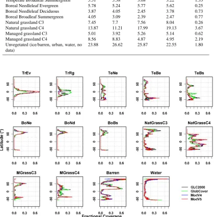
Fig. 2. The latitudinal distribution of the plant functional types for each land-cover dataset. The PFT acronyms correspond to those in Table 2.
were removed to allow the establishment of PFTs wher-ever they were prescribed from the external datasets. In the LPJmL model, diagnostic PFT fractions replaced the variable for maximum annual fraction of photosynthetic absorbed ra-diation (FPAR) while not modifying the vegetation dynamics or physiology modules. Monthly climate data (precipitation,
Fig. 3. Map of the PFT fractions (at 0.5 degrees resolution) from (a) Modis C005 land-cover inputs using the IGBP legend, and (b) GlobCover land-cover inputs using the LCCS legend. The PFT acronyms correspond to those in Table 2.
(Thonicke et al., 2001), was initiated beginning in 1901 and ending in 2005. Managed grasslands were treated as in Bon-deau et al. (2007), with harvest occurring repeatedly during the year when peak leaf area index (LAI) was reached. An-nual GPP and transpiration (from 1956-2005) were regressed with mean annual temperature, total annual photosynthetic active radiation (PAR), and total annual precipitation, from the same time period, to calculate partial correlation coeffi-cients used to interpret the sensitivity of the biogeochemical fluxes to climate.
3 Results
3.1 Uncertainty in global PFT fractions
At the global scale, managed and unmanaged grassland PFTs, which includes croplands and pasture, were most abundant in terms of percent land area (∼30 %), followed by tropical (∼15%), boreal (∼12 %), and temperate PFTs (∼11 %) (Table 8). Classification agreement (Table 8) was lowest (for globally averaged values) for C4 grasses, espe-cially for natural C4 grasslands. Tropical raingreen (TrRg)
Fig. 4. Close-up illustration of PFT fractions for (a) GLC2000, (b) GlobCover, (c) Modis C004 and (d) Modis C005 for Eastern Africa where fine-scale topographic features and their effects on climate zones are apparent.
interior Australia was classified as “open shrublands” by the IGBP MODIS legend (Fig. 3a; higher abundance of TrEv and TrRg compared to Fig. 3b). Our reclassification for the IGBP legend assigned 40 % of this class to woody PFTs, 20 % to grass PFTs and 40 % to barren. In comparison, the LCCS legend reclassifies part of this region as “sparse vegetation”, which we reclassified as 40 % grass PFT and 60 % bare, consistent with the supporting documentation for LCCS (Fig. 3b; lower abundance of TrEv and TrRg). The IGBP “open shrubland” category also includes tundra and permafrost biomes (in addition to the warmer arid regions). Herbaceous cover may be higher in these cooler regions than in “open shrublands” of warm regions (Fig. 3b; NatGrassC3 replaces by BoNe), which suggests that further refinement of shrubland categories could improve differences between land-cover products.
Spatial resolution and the detail of land-cover categories had important effects in intensively managed landscapes. For example, in the Southeastern United States, the Glob-Cover dataset (0.3 km) and LCCS legend (22 classes)
bet-ter distinguished secondary succession vegetation (Fig. 3b; higher abundance of TeNe) (i.e., pine forests from agricul-tural abandonment, Christensen and Peet, 1984). Climatic differences across small gradients were generally detected by the K¨oppen-Geiger classification, despite elevation not being included in the interpolation process. These topographic fea-tures were apparent in the north-south divide along the island of Madagascar (Fig. 4a–d; NatGrassC4 versus TrRg), along the Andes, separating the Amazon rainforests from high-elevation grasslands, as well as in Ethiopia, where the effects of the highland rift-valley corresponded to C3 grasslands in a region mostly surrounded by C4 climate zones (Fig. 4a–d; NatGrassC3).
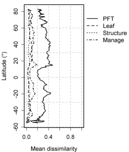
Fig. 5. Latitudinal distributions of mean dissimilarity for the 3 dif-ferent grouping of PFT traits and for all PFTs (described in Meth-ods: Measuring PFT agreement).
and MODIS) for the European Alps. C4 abundance was higher than in Still et al. (2003) who found that globally, C4 vegetation compose∼15 % of terrestrial vegetation (whereas the estimates presented here are closer to∼22 %, Table 8). The higher estimates for C4 grass abundance are due, in part, to differences in the IGBP “grasslands” and LCCS “sparsely vegetated” categories, which corresponded to the LCCS “sparse vegetation” or “barren” categories (Fig. 3a and b; see MGrassC4). For IGBP, “grasslands” were reclassified to 100 % grass cover (Table 6), but for LCCS “sparse vege-tation,” only 40 % grass cover (Table 5).
The disagreement between PFT trait-groups (see cate-gories described in Methods: Measuring PFT agreement), was highest in the tropics (Fig. 5; 20◦N to 20◦S) and for a “hotspot” in the mid-western United States (Fig. 5; 35– 55◦N) resulting from managed versus natural grassland clas-sification. Phenology-type disagreement was also high in the tropics, but in general, structural (physiognomy) observa-tions appear to have high agreement (Fig. 5). In the northern temperate zone, grasslands were more consistently classified as managed, with the exception of mid-western USA, where GlobCover underestimated cropland fraction compared to GLC2000 and MODIS (Fig. 2; MGrassC3). Tropical savan-nas and warm-climate croplands emerged as bands of dis-agreement, because of differences between the IGBP and LCCS classification for natural and managed C4 grassland and shrubland categories. A notable region of high uncer-tainty was the Karakum desert in Central Asia which was
classified as “barren” or “sparse vegetation” in LCCS and as “grassland” in IGBP leading to large differences in estimated PFT fractions (Fig. 6).
3.2 Land cover and the uncertainty of fluxes to climate
In diagnostic mode (with PFT distributions prescribed), global GPP ranged from 130.9 to 134.9 PgC a−1 (averaged over 1996–2005) and transpiration ranged from 43 200 to 44 600 H2O km3a−1. These global values were similar to the prognostic (dynamic vegetation) simulation, using the Hyde dataset for managed grasslands (Klein Goldewijk and Batjes, 1997), which produced values of 131.0 PgC a−1and 39 000 H2O km3a−1. All estimates are close to previous analyses of global carbon Beer et al., 2010) and water fluxes (Gerten et al., 2005). GPP and transpiration sensitivity to climate followed similar patterns observed in previous studies (Ne-mani et al., 2003), with temperature important in northern latitudes, radiation more limiting in the wet tropics, and pre-cipitation a dominant feature globally (Fig. 8a). As in Beer et al. 2010), precipitation was the most important global cli-mate variable controlling GPP (65–70%) and transpiration (58–63 %). The range of uncertainty was similar for either GPP or transpiration sensitivity to climate; with agricultural regions in mid-western USA and Europe, and arid regions in Australia and S. Africa showing high uncertainty in the sensitivity of GPP to precipitation (Fig. 8b). In agricultural regions, the lower fractional coverage of croplands in the GlobCover product led to higher grassland LAI (because of no harvesting), causing higher sensitivity (or correlation co-efficient) to precipitation. In semi-arid regions, the MODIS products led to higher GPP sensitivity to precipitation (Fig-ure 8) because of a higher abundance of woody species (with deeper rooting strategies) unable to compete efficiently for minimal rainfall with grasses that had shallow rooting strate-gies.
4 Discussion
4.1 PFT datasets and themes for improvement
Fig. 6. TMap of mean fractional dissimilarity (0 is complete agreement and 1 is complete disagreement) considering all PFTs using the beta-diversity metric (Eq. 1). Representative grid cells shown in Fig. 7 illustrate the main patterns of clustering and spread of the existing products in comparison to the new PFT products presented here.
Fig. 7. Comparison of the 4 new PFT products to one another and the existing products based on older datasets. The NMDS ordination shows
the degree of differences and clustering of the products (black names) and the major PFT gradients (p <0.05) that explain the differences in
Fig. 8. (a) Partial correlation coefficients (PCC) for modeled GPP to radiation, precipitation, and temperature variable for the MODIS C005 PFT product (b) standard deviation of the PCC for all four land-cover simulations.
The main areas of disagreement were found in regions of intensive land management or in regions where accurate spectral discrimination between similar land cover, but dif-ferent land use, caused classification problems (e.g., cropland and natural grassland). High-disagreement was also found in warm/cool arid regions where land-cover categories were ei-ther too broadly defined or because different legend types had conflicting tree-cover thresholds to define forest vegetation. Previous studies have also observed that dryland systems, which include heterogeneous mixtures of grasslands, crop-lands and savanna shrubcrop-lands, feature as prominent zones of disagreement (Giri et al., 2005; Herold et al., 2008; Fritz and See, 2008). Our results confirm that this disagreement scales to PFT groupings and contributes a large part of the land-surface process uncertainty for GPP and transpiration sensitivity to climate (Fig. 9).
Much of this disagreement results from differences in the classification for forest land; the LCCS definition for forest is an area with more than 15 % tree cover, whereas IGBP uses a 60 % tree-cover threshold. Consequently, the MODIS prod-uct has a much larger fraction of (non-forest) shrubland and savanna systems, which are categorized as various “open” or “closed” forest types in GLC2000 and GLOBCOVER, Ta-bles 4 and 6. Such problems stem from defining forest struc-ture from forest cover, which may be overcome with new developments in satellite-based lidar, which can successfully provide measurements of tree height and vertical structure at global extents (Lefsky, 2010). Overlap of cool or warm arid-land categories (i.e., grassarid-land, shrubarid-land, barren), also in-troduced error in deserts and tundra regions, where broadly
defined categories could be improved by including climate information. Arid-regions have large global coverage and re-cent work suggests that these ecosystems have a significant influence on global biogeochemistry and the climate system itself via biophysical properties (Rotenberg and Yakir, 2010), hence a better understanding of their distribution could con-tribute to reducing uncertainty of global climate processes.
Fig. 9. Cumulative partial correlation between GPP and precipitation using the same approach as described in Beer et al. (2010). Zones correspond to TRANSCOM 3 biome regions (Gurney et al., 2003), and legend colors red for GLC2000, green for GlobCover, light blue for Modis v4, and dark blue for Modis v5.
Our analysis suggests that the PFT uncertainties could be reduced by using land-cover data based on high to moderate-spatial resolution and a larger number of legend categories (as in GlobCover). For example, the more detailed LCCS legend was better able to handle dry-land classifications than the coarser IGBP legend and GlobCover appears to classify heterogeneous landscapes well. Future versions of MODIS land-cover data are expected to include the LCCS legend (Friedl et al., 2010), which in addition, should further reduce errors from user-based reclassification necessary for land-cover product comparisons.
4.2 Application with Earth System Models
approach for hypothesis testing and linkage to remote sens-ing will remain important. Finer resolution categories of crop types has been shown to be important for global bio-geochemical cycling (Bondeau et al., 2007) but crop types or crop cover (or pasture) is not easily distinguished in the global land-cover datasets, highlighting the importance of integrated land-cover mapping approaches. Managed grass-land categories can be subdivided using regional statistics on crop use, similar to methods described by Ramankutty et al. (1998), but many earth system models are at the early stages of incorporating crop functional types.
By forcing LPJmL with diagnostic PFT fractions we were able to illustrate the utility of ensembles of land-cover ap-proaches and the application of diagnostic datasets. Interest-ingly, global estimates of GPP and ET were similar, regard-less of land cover, confirming studies conducted at continen-tal scales (Jung et al., 2007). However, we show that there are large regional differences, 20–30 %, in the sensitivity of biogeochemical fluxes to climate that are directly linked to land-cover uncertainty. High-PFT uncertainty did not always correspond to high biogeochemical cycling uncertainty (e.g., wet tropics), illustrating that propagated errors may differ from the initial condition agreement and that the choice of evaluation metric is important. These PFT datasets have ap-plications beyond ESM modeling and can be integrated with bottom-up studies, include accounting methods for evaluat-ing carbon stocks (Kindermann et al., 2008), or as base-maps that can inform biodiversity-patterns related to biogeography (Loucks et al., 2008).
Acknowledgements. B. Poulter acknowledges funding from an FP7
Marie Curie Incoming International Fellowship (Grant Number 220546). NE Zimmermann and H Lischke acknowledge support through the FP6 and FP7 projects ECOCHANGE (GOCE-CT-2007-036866) and MOTIVE (ENV-CT-2009-226544). E Hodson acknowledges support from the MAIOLICA Project. The authors are grateful for the development and distribution of the remote sensing datasets from European Commission’s Joint Research Cen-ter, Ispra, Italy, the European Space Agency, and Boston University.
Edited by: A. Stenke
The publication of this article is financed by CNRS-INSU.
References
Alton, P., Fisher, R. A., Los, S. O., and Williams, M.: Simulations of global evapotranspiration using semiempirical and mechanis-tic schemes of plant hydrology, Global Biogeochem. Cy., 23, doi:10.1029/2009GB003540, 2009.
Arino, O., Bicheron, P., Achard, F., Latham, J., Witt, R., and Weber, J. L.: GLOBCOVER The most detailed portrait of Earth, ESA Bulletin-European Space Agency, 136, 24–31, 2008.
Baker, I. T., Prihodko, L., Denning, A. S., Goulden, M. L., Miller, S. D., and da Rocha, H. R.: Seasonal drought stress in the Ama-zon: Reconciling models and observations, J. Geophys. Res., 113, doi:10.1029/2007JG000644, 2008.
Bartholome, E. and Belward, A. S.: GLC2000: a new approach to global land cover mapping from Earth observation data, Int. J. Remote Sens., 26, 1959–1977, 2005.
Beer, C., Reichstein, M., Tomelleri, E., Ciais, P., Jung, M., Carval-hais, N., R¨odenbeck, C., Arain, M. A., Baldocchi, D., Bonan, G., Bondeau, A., Cescatti, A., Lasslop, G., Lindroth, A., Lomas, M., Luyssaert, S., Margolis, H., Oleson, K. W., Roupsard, O., Veenendaal, E., Viovy, N., Williams, C., Woodward, F. I., and Papale, D.: Terrestrial gross carbon dioxide uptake: Global dis-tribution and covariation with climate, Science, 329, 834–838, 2010.
Bonan, G. B., Levis, S., Kergoat, L., and Oleson, K. W.: Land-scapes as patches of plant functional types: An integrating con-cept for climate and ecosystem models, Global Biogeochem. Cy., 16, doi:10.1029/2000GB001360, 2002.
Bondeau, A., Smith, P. C., Zaehle, S., Schaphoff, S., Lucht, W., Cramer, W., Gerten, D., Lotze-Campen, H., M¨uller, C., Reich-stein, M., and Smith, B.: Modelling the role of agriculture for the 20th century global carbon balance, Glob. Change Biol., 13, 679–706, 2007.
Christensen, N. L. and Peet, R. K.: Convergence during secondary forest succession, J. Ecol., 65, 25–36, 1984.
Collatz, G. J., Berry, J. A., and Clark, J. S.: Effects of climate and
atmospheric CO2 partial pressure on the global distribution of
C4 grasses: Present, past, and future, Oecologia, 114, 441–454, 1998.
DeFries, R., Hansen, M. C., Townshend, J. R. G., Janetos, A. C., and Loveland, T. R.: A new global 1-km dataset of percentage tree cover derived from remote sensing, Glob. Change Biol., 6, 247–254, 2000.
Dickinson, R. E., Oleson, K. W., Bonan, G. B., Hoffman, F., Thorn-ton, P. E., Vertenstein, M., Yang, Z. L., and Zeng, X.: The Com-munity Land Model and its climate statistics as a component of the Community Climate System Model, J. Climate, 19, 2302– 2324, 2006.
Foley, J. A., Defries, R., Asner, G. P., Barford, C., Bonon, G., Car-penter, S. R., Chapin, F. S., Coe, M. T., Daily, G. C., Gibbs, H. K., Helkowski, J. H., Holloway, T., Howard, E. A., Kucharik, C. J., Monfreda, C., Patz, J. A., Prentice, I. C., Ramankutty, N., and Snyder, P. K.: Global consequences of land use, Science, 309, 570–574, 2005.
Friedl, M. A., Sulla-Menashe, D., Tan, B., Schneider, A., Ra-mankutty, N., Sibley, A., and Huang, X.: MODIS Collection 5 Global Land Cover: Algorithm refinements and characterization of new datasets, Remote Sens. Environ., 114, 168–182, 2010. Fritz, S. and See, L.: Identifying and quantifying uncertainty and
spatial disagreement in the comparison of Global Land Cover for different applications, Global Change Biol., 14, 1057–1075, 2008.
Gerten, D., Hoff, H., Bondeau, A., Lucht, W., Smith, P., and Zaehle, S.: Contemporary “green” water flows: Simulations with a dy-namic global vegetation and water balance model, Phys. Chem. Earth, 30, 334–338, 2005.
Giri, C., Zhu, Z., and Reed, B.: A comparative analysis of the Global Land Cover 2000 and MODIS land cover data sets, Re-mote Sens. Environ., 94, 123–132, 2005.
Gurney, K. R., Law, R. M., Denning, A. S., Rayner, P., Baker, D., Bousquet, P., Bruhwiler, L., Chen, Y. H., Ciais, P., Fan, S., Fung, I. Y., Gloor, M., Heimann, M., Higuchi, K., John, J., Kowal-czyk, E., Maki, T., Maksyutov, S., Peylin, P., Prather, M., Pak, B., Sarmiento, J., Taguchi, S., Takahashi, T., and Yuen, C. W.:
TransCom 3 CO2inversion intercomparison: 1. Annual mean
control results and sensitivity to transport and prior flux informa-tion, Tellus, 55B, 555–579, 2003.
Haberl, H., Erb, K. H., Krausmann, F., Gaube, V., Bondeau, A., Plutzar, C., Gingrich, S., Lucht, W., and Fischer-Kowalski, M.: Quantifying and mapping the human appropriation of net pri-mary production in earth’s terrestrial ecosystems, P. National Academy of Science, 104, 12942–12947, 2007.
Herold, M., Mayaux, P., Woodcock, C. E., Baccini, A., and Schmul-lius, C.: Some challenges in global land cover mapping: An as-sessment of agreement and accuracy in existing 1 km datasets, Remote Sens. Environ., 112, 2538–2556, 2008.
Hugh, E. D., Belward, A., De Miranda, E. E., Di Bella, C. M., Gond, V., Huber, O., Jones, S., Sgrenzaroli, M., and Fritz, S.: A land cover map of South America, Glob. Change Biol., 10, 731–744, 2004.
Jung, M., Henkel, K., Herold, M., and Churkina, G.: Exploiting synergies of global land cover products for carbon cycle model-ing, Remote Sens. Environ., 101, 534–553, 2006.
Jung, M., Vetter, M., Herold, M., Churkina, G., Reichstein, M., Za-ehle, S., Ciais, P., Viovy, N., Bondeau, A., Chen, Y., Trusilova, K., Feser, F., and Heimann, M.: Uncertainties of modeling gross primary productivity over Europe: A systematic study on the ef-fects of using different drivers and terrestrial biosphere models, Glob. Biogeochem. Cy., 21, doi:10.1029/2006GB002915, 2007. Kindermann, G., McCallum, I., Fritz, S., and Obersteiner, M.: A Global Forest Growing Stock, Biomass and Carbon Map Based on FAO Statistics, Silva Fennica, 42, 387–396, 2008.
Kleidon, A., Adams, J., Pavlick, R., and Reu, B.: Simulated geo-graphic variations of plant species richness, evenness and abun-dance using climatic constraints on plant functional diversity, En-viron. Res. Lett., 4, 014007, doi:10.1088/1748-9326/4/1/014007, 2009.
Klein Goldewijk, K. and Batjes, J. J.: A hundred year (1890–1990) database for integrated environmental assessments (HYDE, ver-sion 1.1), Bilthoven, the Netherlands, 1997.
Klein Goldewijk, K., van Drecht, G., and Bouwman, A. F.: Map-ping contemporary global cropland and grassland distributions on a 5 x 5 minute resolution, J. Land Use Sci., 2, 167–190, 2007.
Kobayashi, H. and Dye, D. G.: Atmospheric conditions for mon-itoring the long-term vegetation dynamics in the Amazon using normalized difference vegetation index, Remote Sens. Environ., 97, 519–525, 2005.
K¨oppen, W.: Das geographisca System der Klimate, in: Handbuch der Klimatologie, edited by: K¨oppen, W., and Geiger, G., 1. C. Gebr, Borntraeger, 1–44, 1936.
Krinner, G., Viovy, N., de Noblet-Ducoudr´e, N., Oge´e, J., Polcher, J., Friedlingstein, P., Ciais, P., Sitch, S., and Prentice, I. C.: A dynamic global vegetation model for studies of the cou-pled atmosphere-biosphere system, Glob. Biogeochem. Cy., 19, GB1015, doi:1010.1029/2003GB002199, 2005.
Lapola, D. M., Oyama, M. D., Nobre, C. A., and Sampaio, G.: A new world natural vegetation map for global change studies, Annals of the Brazilian Academy of Science, 80, 397–408, 2008. Lawrence, P. J. and Chase, T. N.: Representing a MODIS Consis-tent Land Surface in the Community Land Model (CLM 3.0): Part 1 Generating MODIS Consistent Land Surface Parameters, J. Geophys. Res., 112, doi:10.1029/2006JG000168, 2007. Lefsky, M. A.: A global forest canopy height map from the
Moderate Resolution Imaging Spectroradiometer and the Geo-science Laser Altimeter System, Geophys. Res. Lett., 37, doi:10.1029/2010GL043622, 2010.
Legates, D. R. and Wilmott, C. J.: Mean seasonal and spatial vari-ability in global surface air temperature, Theor. Appl. Climatol., 41, 11–21, 1990.
Legendre, P., Borcard, D., and Peres-Neto, P. R.: Analyzing beta diversity: Partitioning the spatial variation of community com-position data, Ecol. Monogr., 75, 435–450, 2005.
Loucks, C. J., Ricketts, T. H., Naidoo, R., Lamoreux, J. F., and Hoekstra, J. M.: Explaining the global pattern of protected area coverage: relative importance of vertebrate biodiversity, human activities and agricultural suitability, J. Biogeogr., 35, 1337– 1348, 2008.
Matthews, E.: Global vegetation and land use: New high-resolution data bases for climate studies, J. Clim. Appl. Meteorol., 22, 474– 487, 1983.
Mitchell, C. D. and Jones, P.: An improved method of constructing a database of monthly climate observations and associated high-resolution grids, Int. J. Climatol., 25, 693–712, 2005.
Morton, D. C., DeFries, R. S., Shimabukuro, Y. E., Anderson, L. O., Arai, E., del Bon Espirito-Santo, F., Freitas, R., and Morisette, J. T.: Cropland expansion changes deforestation dynamics in the southern Brazilian Amazon, P. National Academy of Science, 103, 14637–14641 2006.
Nemani, R. R., Keeling, C. D., Hashimoto, H., Jolly, W. M., Piper, S. C., Tucker, C. J., Myneni, R. B., and Running, S.: Climate-Driven Increases in Global Terrestrial Net Primary Production from 1982 to 1999, Science, 300, 1560–1563, 2003.
New, M., Lister, D., Hulme, M., and Makin, I.: A high-resolution data set of surface climate over global land areas, Clim. Res., 21, 1-25, 2002.
Oki, T. and Kanae, S.: Global hydrological cycles and world water resources, Science, 313, 1068–1072, 2006.
Olson, J., Watts, J. A., and Allison, L. J.: Carbon in Live Vegetation of Major World Ecosystems, ORNL-5862, Oak Ridge National Laboratory, Oak Ridge, Tennessee, 164 pp., 1983.
Earth Syst. Sci., 11, 1633–1644, doi:10.5194/hess-11-1633-2007, 2007.
Plummer, S.: Perspectives on combining ecological process models and remotely sensed data, Ecol. Model., 129, 169–186, 2000. Poulter, B. and Cramer, W.: Satellite remote sensing of tropical
forest canopies and their seasonal dynamics, Int. J. Remote Sens., 30, 6575–6590, 2009.
Poulter, B., Heyder, U., and Cramer, W.: Modelling the sensitivity of the seasonal cycle of GPP to dynamic LAI and soil depths in tropical rainforests, Ecosystems, 12, 517–533, 2009.
Prentice, I. C., Cramer, W., Harrison, S. P., Leemans, R., Monserud, R. A., and Soloman, A. M.: A global biome model based on plant physiology and dominance, soil properties and climate, J. Biogeogr., 19, 117–134, 1992.
Quaife, T., Quegan, S., Disney, M., Lewis, P., Lomas, M. R., and Woodward, F. I.: Impact of land cover uncertainties on esti-mates of biospheric carbon fluxes, Glob. Biogeochem.l Cy., 22, doi:10.1029/2007GB003097, 2008.
Ramankutty, N. and Foley, J. A.: Characterizing patterns of global land use: An analysis of global croplands data, Glob. Bio-geochem. Cy., 12, 667–685, 1998.
Rotenberg, E. and Yakir, D.: Contribution of semi-arid forests to the climate system, Science, 327, 451–454, 2010.
Running, S., Loveland, T. R., Pierce, L. L., Nemani, R. R., and Hunt, E. R.: A remote sensing based vegetation classification logic for global land cover analysis, Remote Sens. Environ., 51, 39–48, 1995.
Saleska, S. R., Didan, K., Huete, A. R., and da Rocha, H. R.: Ama-zon forests green-up during 2005 drought, Science, 318, 612, 2007.
Samanta, A., Ganguly, S., Hashimoto, H., Devadiga, S., Vermote, E. F., Knyazikhin, Y., Nemani, R. R., and Myneni, R. B.: Amazon forests did not green-up during the 2005 drought, Geophys. Res. Lett., 37, doi:10.1029/2009GL042154 2010.
Scheiter, S. and Higgins, S. I.: Impacts of climate change on the vegetation of Africa: an adaptive dynamic vegetation modelling approach, Glob. Change Biol., 15, 2224–2246, 2009.
Schimel, D. S., House, J. I., Hibbard, K., Bousquet, P., Ciais, P., Peylin, P., Braswell, B., Apps, M. J., Baker, D., Bondeau, A., Canadell, J. G., Churkina, G., Cramer, W., Denning, A. S., Field, C. B., Friedlingstein, P., Goodale, C., Heimann, M., Houghton, R. A., Melillo, J. M., Moore III, B., Murdiyarso, D., Noble, I. P., S.W., Prentice, I. C., Raupach, M., Rayner, P., Scholes, R. J., Steffen, W., and Wirth, C.: Recent patterns and mechanisms of carbon exchange by terrestrial ecosystems, Nature, 414, 169– 172, 2001.
Sitch, S., Smith, B., Prentice, I. C., Arneth, A., Bondeau, A., Cramer, W., Kaplan, J. O., Levis, S., Lucht, W., Sykes, M. T., Thonicke, K., and Venevsky, S.: Evaluation of ecosystem dy-namics, plant geography and terrestrial carbon cycling in the LPJ dynamic global vegetation model, Glob. Change Biol., 9, 161– 185, 2003.
Smith, T. M., Shugart, H. H., and Woodward, F. I.: Plant functional types: their relevance to ecosystem properties and global change, Cambridge University Press, New York, 369 pp., 1997.
Sterling, S. and Ducharne, A.: Comprehensive data set of global land cover change for land surface model applications, Glob. Biogeochem. Cy., 22, doi:10.1029/2007GB002959, 2008. Still, C. J., Berry, J. A., Collatz, G. J., and DeFries, R.: Global
distribution of C3 and C4 vegetation: Carbon cycle implications, Glob. Biogeochem. Cy., 17, doi:10.1029/2001GB001807, 2003. Sun, W., Liang, S., Xu, G., Fang, H., and Dickinson, R. E.: Map-ping plant functional types from MODIS data using multisource evidential reasoning, Remote Sens. Environ., 112, 1010–1024, 2008.
Thonicke, K., Venevsky, S., Sitch, S., and Cramer, W.: The role of fire disturbance for global vegetation dynamics: coupling fire into a Dynamic Global Vegetation Model, Global Ecol. Bio-geogr., 10, 661–677, 2001.
Ustin, S. L. and Gamon, J. A.: Remote sensing of plant functional types, New Phytologist, 186, 795–816, 2010.
Verant, S., Laval, K., Polcher, J., and De Castro, M.: Sensitivity of the continental hydrological cycle to the spatial resolution over the Iberian Peninsula, J. Hydrometeorol., 5, 267–285, 2004. Wang, A., Price, D. T., and Arora, V. K.: Estimating changes in
global vegetation cover (1850-2100) for use in climate mod-els, Global Biogeochem. Cy., 20, doi:10.1029/2005GB002514, 2006.
Whittaker, R. H.: Evolution and measurement of species diversity, Taxon, 21, 213–251, 1972.